
Real-Time 3D Reconstruction Pipeline for Room-Scale, Immersive, Medical Teleconsultation

 , , , and
Abstract
:1. Introduction
2. Related Work
2.1. Real-Time Dynamic Surface Reconstruction
2.2. Isosurface Extraction
2.3. Mesh Simplification with Dual Contouring
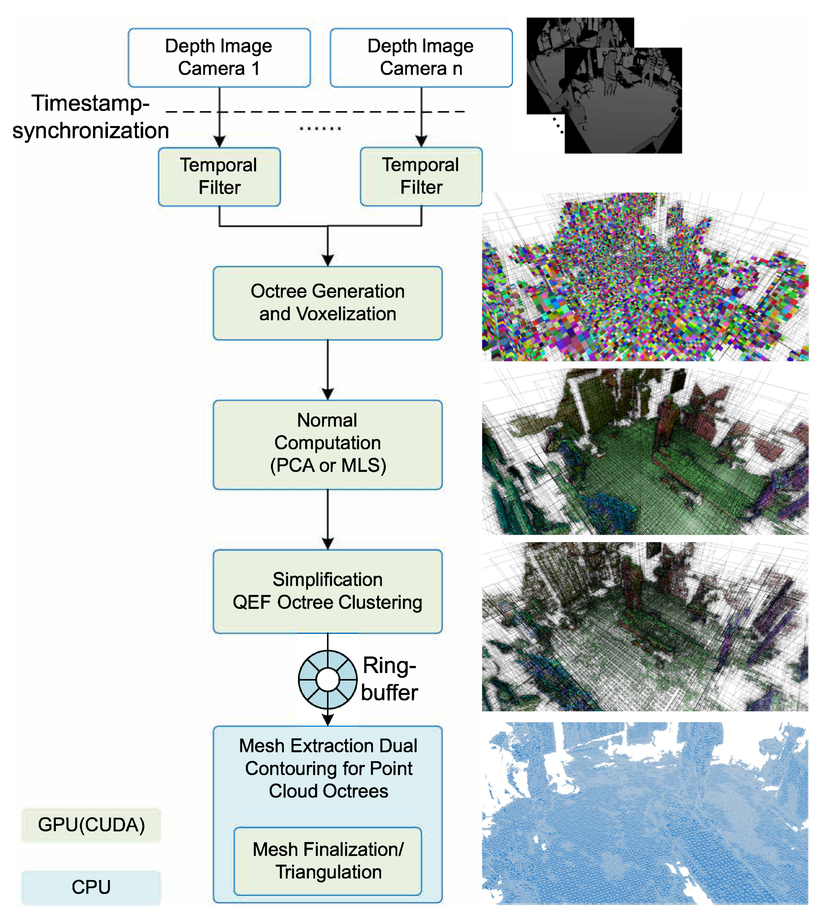
3. Pipeline Overview
3.1. Octree Generation and Voxelization
3.2. Surface Sample and Normal Estimation
3.3. Simplification via Octree-Based Vertex Clustering
3.4. Dual Contouring for Point Clouds
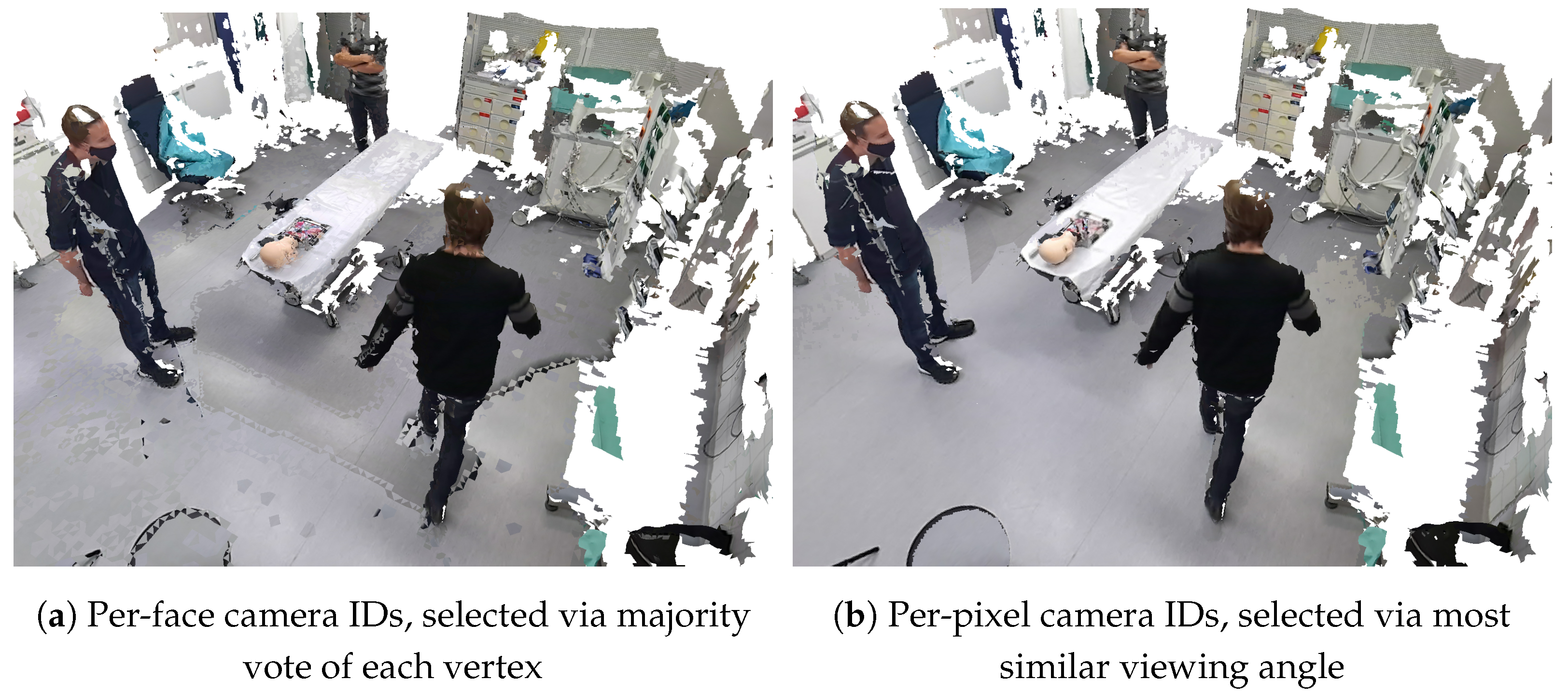
3.5. Textured Rendering
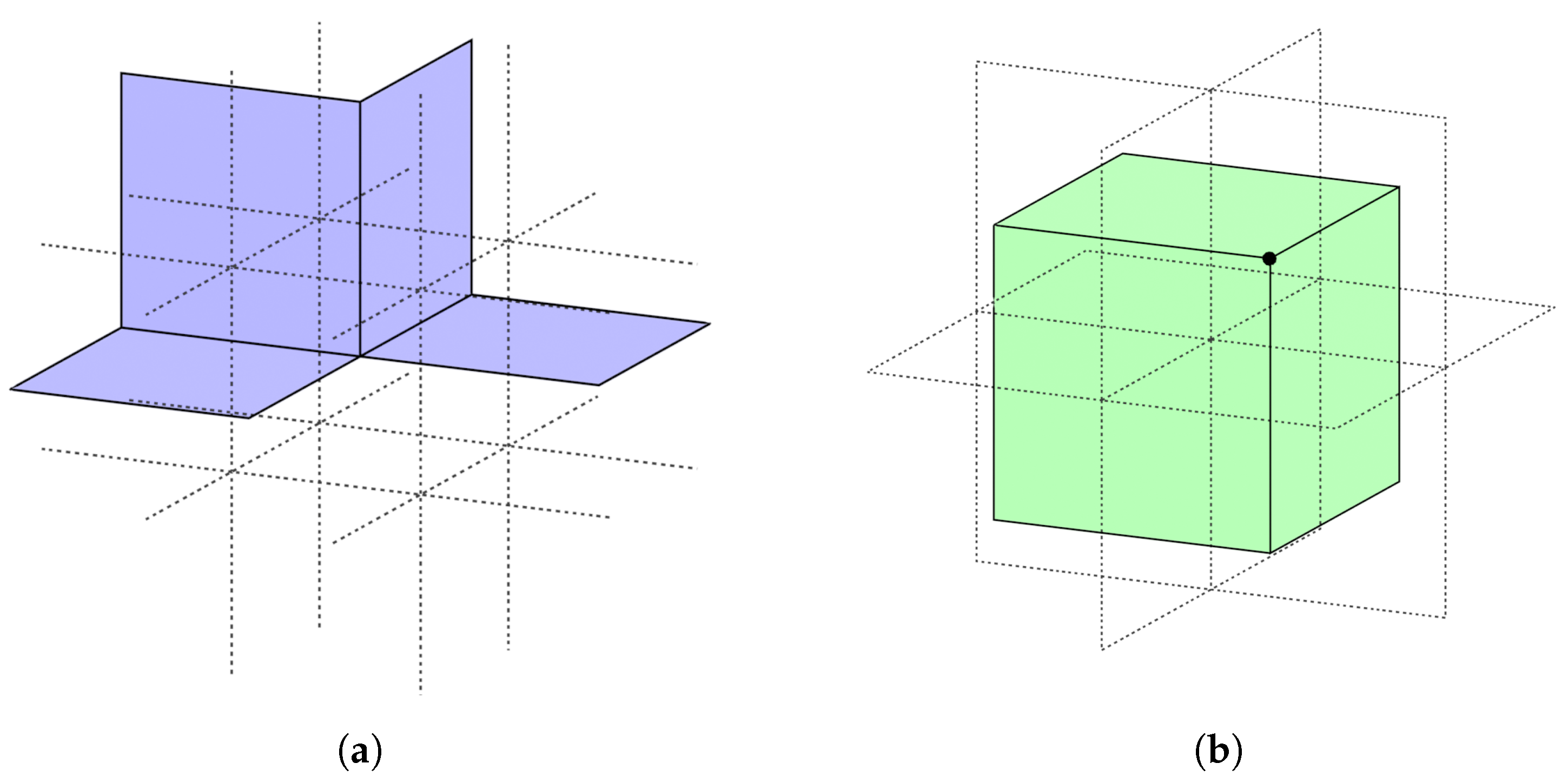
4. Dual Contouring for Voxelized Point Clouds
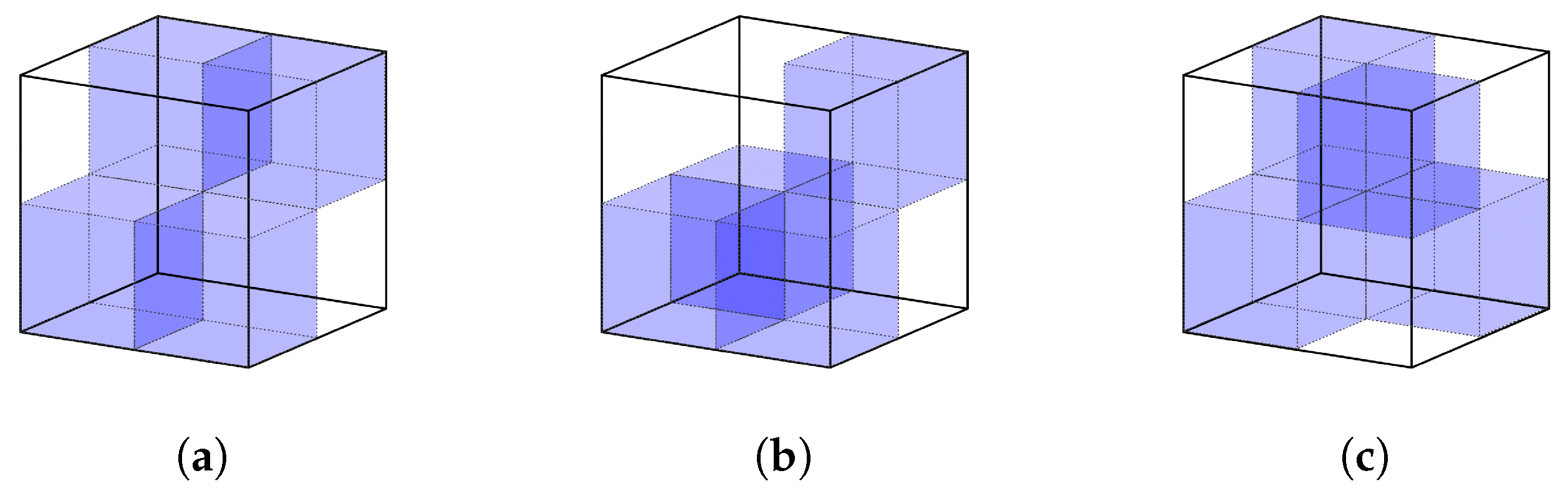
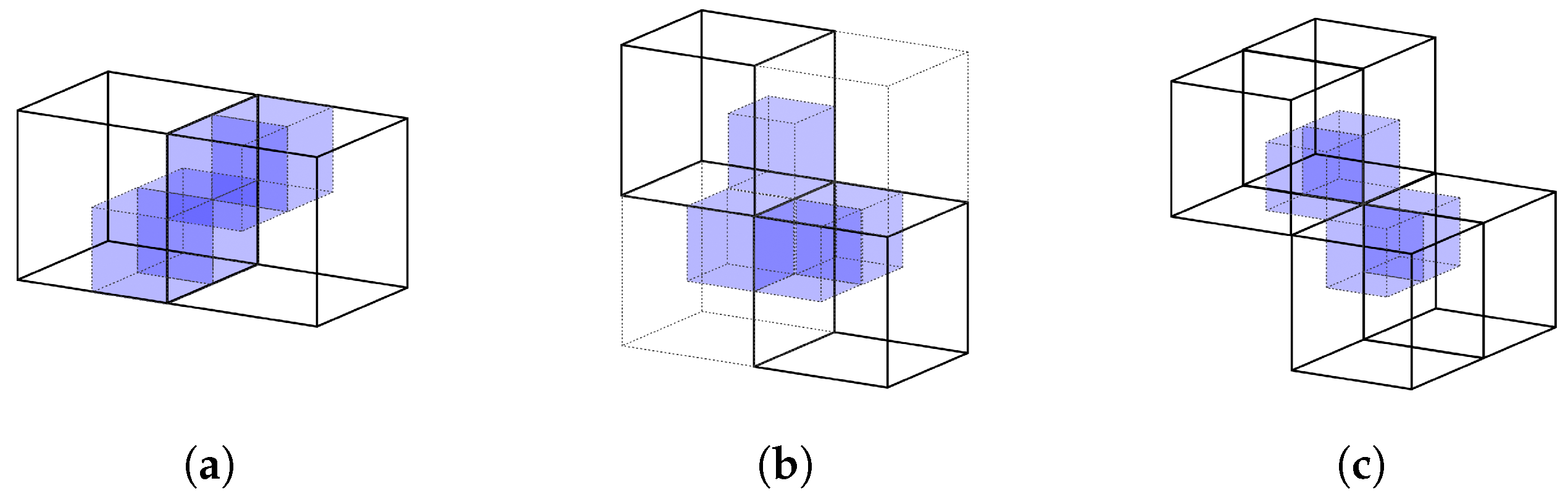
4.1. Extension for Diagonal Connections
4.2. Connectivity Properties and Interior Mesh Generation

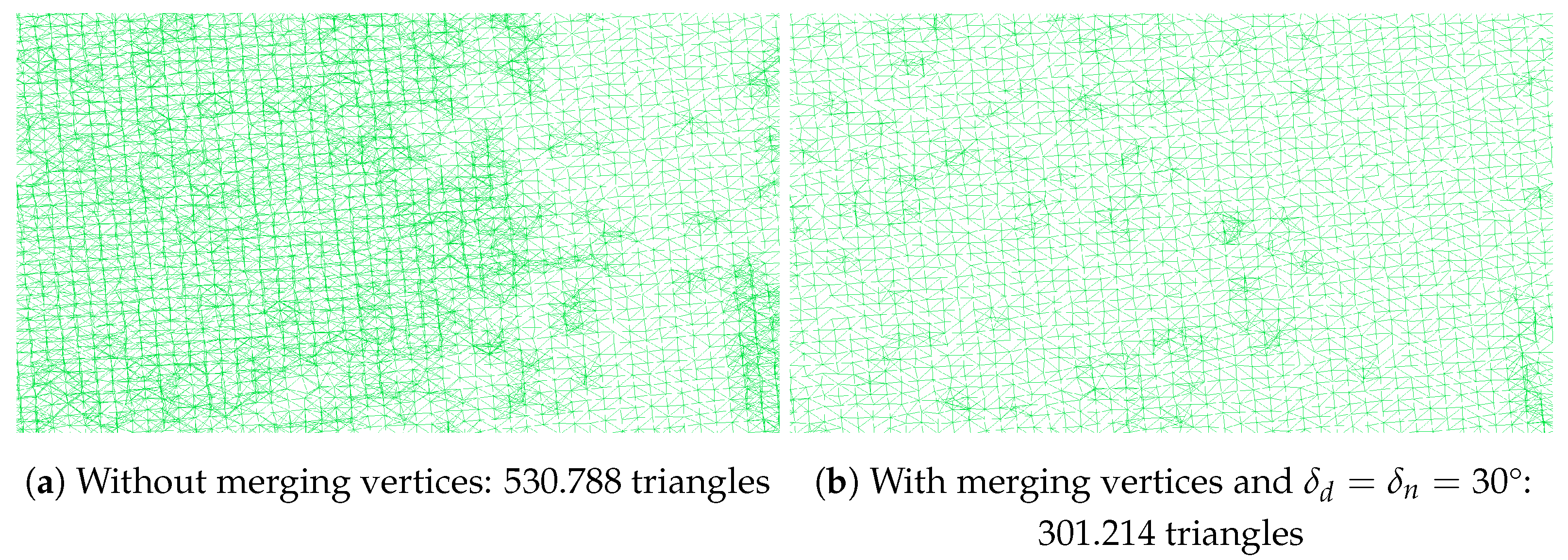
5. Topology and Silhouette-Preserving Simplification
5.1. Preventing Interior Faces
5.2. Silhouette Preservation
6. Evaluation
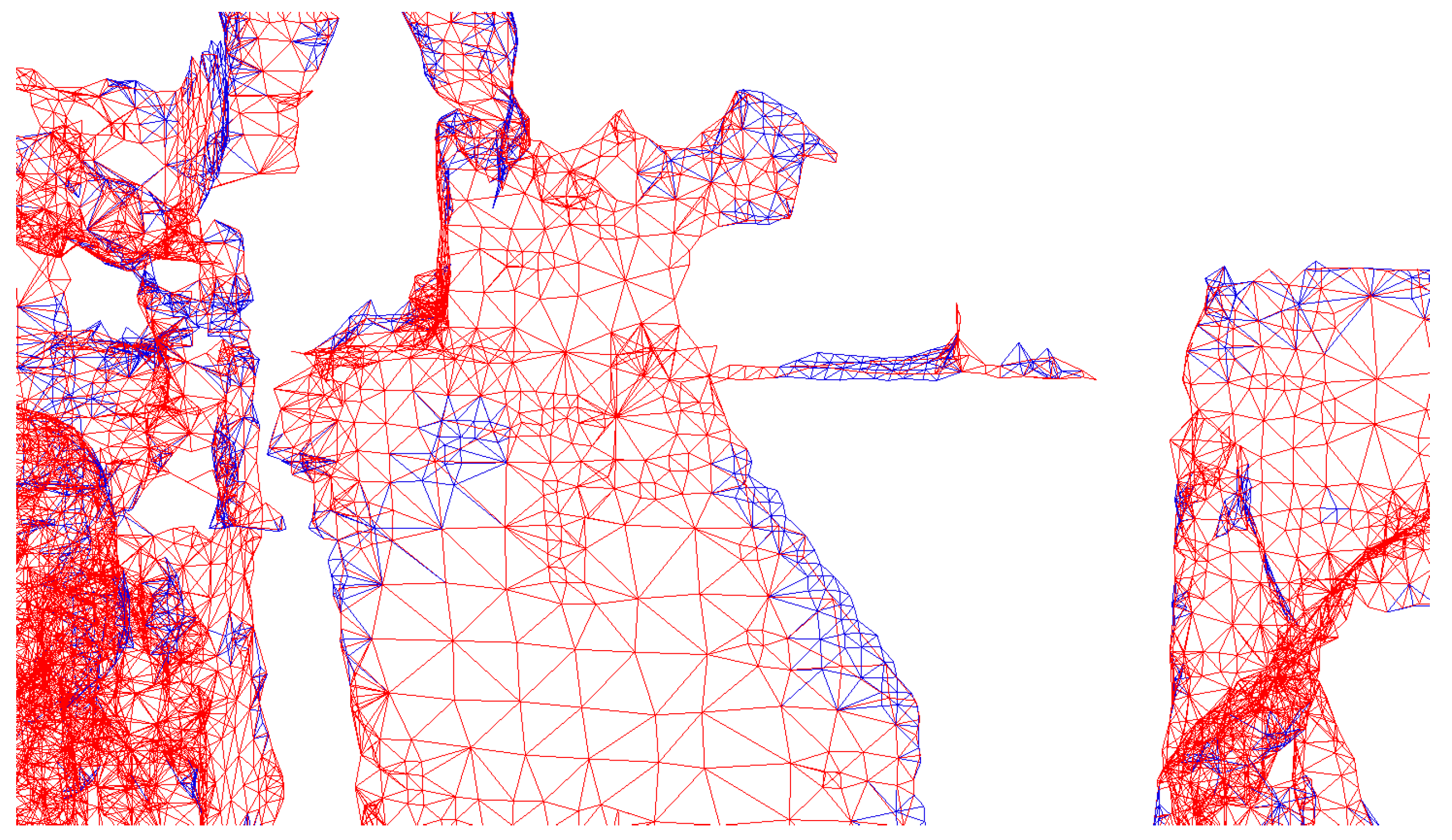
6.1. Comparison with Existing Offline Methods
6.2. Simplification Characteristics
6.3. Performance Characteristics
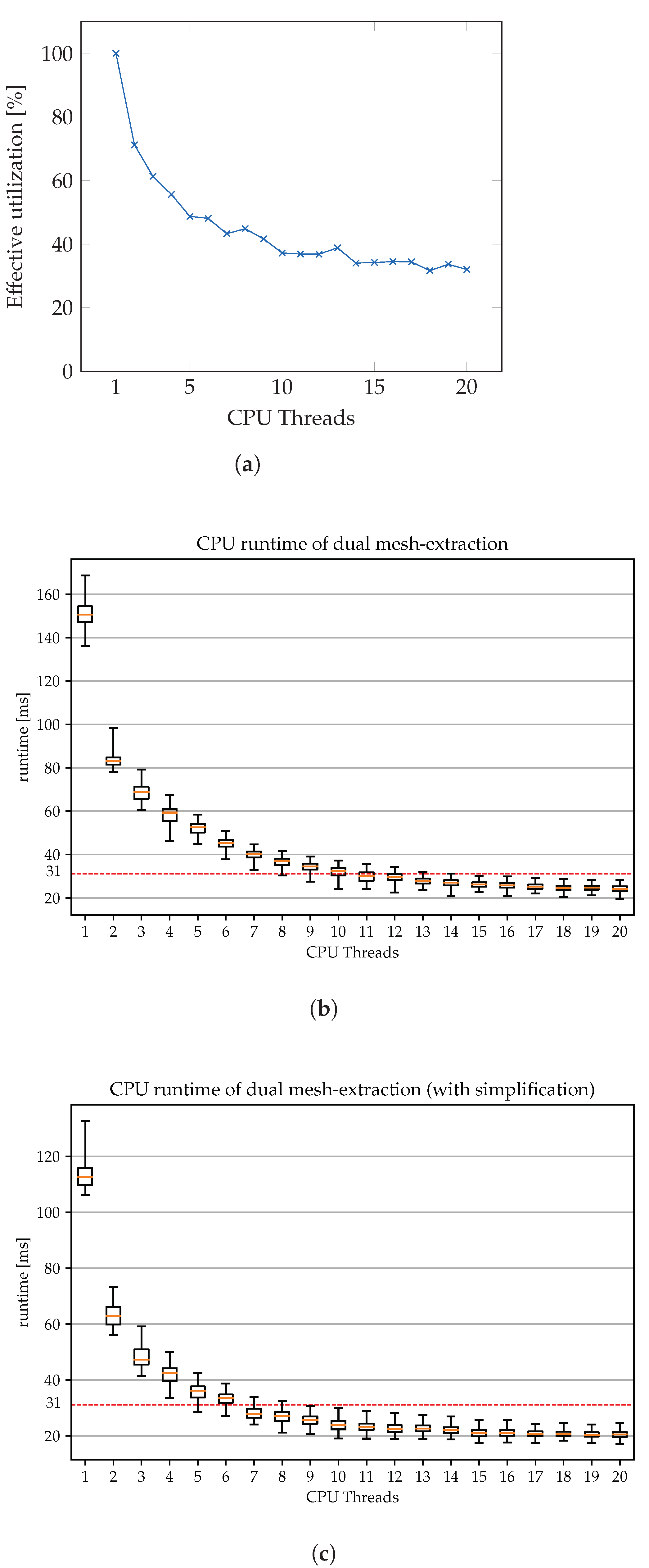
6.3.1. CPU Scaling
6.3.2. Full System Performance
7. Discussion
8. Conclusions and Future Work
Author Contributions
Funding
Institutional Review Board Statement
Informed Consent Statement
Data Availability Statement
Conflicts of Interest
References
- Steuer, J. Defining Virtual Reality: Dimensions Determining Telepresence. J. Commun. 1992, 42, 73–93. [Google Scholar] [CrossRef]
- Weibel, N.; Gasques, D.; Johnson, J.; Sharkey, T.; Xu, Z.R.; Zhang, X.; Zavala, E.; Yip, M.; Davis, K. Artemis: Mixed-reality Environment for Immersive Surgical Telementoring. In Proceedings of the Extended Abstracts of the 2020 CHI Conference on Human Factors in Computing Systems, Honolulu, HI, USA, 25–30 April 2020; pp. 1–4. [Google Scholar]
- Stotko, P.; Krumpen, S.; Hullin, M.B.; Weinmann, M.; Klein, R. SLAMCast: Large-Scale, Real-Time 3D Reconstruction and Streaming for Immersive Multi-Client Live Telepresence. IEEE Trans. Vis. Comput. Graph. 2019, 25, 2102–2112. [Google Scholar] [CrossRef] [PubMed]
- Dou, M.; Khamis, S.; Degtyarev, Y.; Davidson, P.; Fanello, S.R.; Kowdle, A.; Escolano, S.O.; Rhemann, C.; Kim, D.; Taylor, J.; et al. Fusion4d: Real-time performance capture of challenging scenes. ACM Trans. Graph. (ToG) 2016, 35, 1–13. [Google Scholar] [CrossRef]
- Maimone, A.; Fuchs, H. Encumbrance-free telepresence system with real-time 3D capture and display using commodity depth cameras. In Proceedings of the 2011 10th IEEE International Symposium on Mixed and Augmented Reality, Basel, Switzerland, 26–29 October 2011; IEEE: Manhattan, NY, USA, 2011; pp. 137–146. [Google Scholar]
- Fuchs, H.; Bishop, G.; Arthur, K.; McMillan, L.; Bajcsy, R.; Lee, S.; Farid, H.; Kanade, T. Virtual Space Teleconferencing Using a Sea of Cameras. In Proceedings of the 1st International Conference on Medical Robotics and Computer Assisted Surgery (MRCAS ’94), Pittsburgh, PA, USA, 22 September 1994; pp. 161–167. [Google Scholar]
- Fuchs, H.; State, A.; Bazin, J.C. Immersive 3D Telepresence. Computer 2014, 47, 46–52. [Google Scholar] [CrossRef]
- Beck, S.; Kunert, A.; Kulik, A.; Froehlich, B. Immersive Group-to-Group Telepresence. IEEE Trans. Vis. Comput. Graph. 2013, 19, 616–625. [Google Scholar] [CrossRef] [PubMed]
- Beck, S.; Froehlich, B. Volumetric Calibration and Registration of Multiple RGBD-sensors into a Joint Coordinate System. In Proceedings of the 2015 IEEE Symposium on 3D User Interfaces (3DUI), Arles, France, 23–24 March 2015; pp. 89–96. [Google Scholar]
- Zwicker, M.; Pfister, H.; van Baar, J.; Gross, M. Surface Splatting. In Proceedings of the 28th Annual Conference on Computer Graphics and Interactive Techniques, New York, NY, USA, 1 August 2001; SIGGRAPH ’01. pp. 371–378. [Google Scholar] [CrossRef]
- Kawata, H.; Kanai, T. Image-Based Point Rendering for Multiple Range Images. In Proceedings of the 2nd International Conference on Information Technology and Applications, Salt Lake City, UT, USA, 15–17 June 2004; pp. 478–483. [Google Scholar]
- Calakli, F.; Taubin, G. SSD: Smooth signed distance surface reconstruction. Comput. Graph. Forum 2011, 30, 1993–2002. [Google Scholar] [CrossRef]
- Söderholm, H.M.; Sonnenwald, D.H.; Cairns, B.; Manning, J.E.; Welch, G.F.; Fuchs, H. The Potential Impact of 3d Telepresence Technology on Task Performance in Emergency Trauma Care. In Proceedings of the 2007 International ACM Conference on Supporting Group Work, New York, NY, USA, 4–7 November 2007; GROUP ’07. pp. 79–88. [Google Scholar] [CrossRef]
- Welch, G.; Sonnenwald, D.H.; Fuchs, H.; Cairns, B.; Mayer-Patel, K.; Yang, R.; Towles, H.; Ilie, A.; Krishnan, S.; Söderholm, H.M.; et al. Remote 3D medical consultation. In Virtual Realities; Springer: Berlin/Heidelberg, Germany, 2011; pp. 139–159. [Google Scholar]
- Meerits, S.; Thomas, D.; Nozick, V.; Saito, H. FusionMLS: Highly dynamic 3D reconstruction with consumer-grade RGB-D cameras. Comput. Vis. Media 2018, 4, 287–303. [Google Scholar] [CrossRef]
- Lorensen, W.E.; Cline, H.E. Marching Cubes: A High Resolution 3D Surface Construction Algorithm. SIGGRAPH Comput. Graph. 1987, 21, 163–169. [Google Scholar] [CrossRef]
- Ju, T.; Losasso, F.; Schaefer, S.; Warren, J. Dual contouring of hermite data. In Proceedings of the 29th Annual Conference on Computer Graphics and Interactive Techniques, San Antonio, TX, USA, 23–26 July 2002; pp. 339–346. [Google Scholar]
- Orts-Escolano, S.; Rhemann, C.; Fanello, S.; Chang, W.; Kowdle, A.; Degtyarev, Y.; Kim, D.; Davidson, P.L.; Khamis, S.; Dou, M.; et al. Holoportation: Virtual 3D Teleportation in Real-Time. In Proceedings of the 29th Annual Symposium on User Interface Software and Technology, New York, NY, USA, 16–19 October 2016; UIST ’16. pp. 741–754. [Google Scholar]
- Pejsa, T.; Kantor, J.; Benko, H.; Ofek, E.; Wilson, A. Room2Room: Enabling Life-Size Telepresence in a Projected Augmented Reality Environment. In Proceedings of the 19th ACM Conference on Computer-Supported Cooperative Work & Social Computing, New York, NY, USA, 27 February–2 March 2016; CSCW ’16. pp. 1716–1725. [Google Scholar]
- Hartley, R.; Zisserman, A. Multiple View Geometry in Computer Vision, 2nd ed.; Cambridge University Press: New York, NY, USA, 2003. [Google Scholar]
- Collet, A.; Chuang, M.; Sweeney, P.; Gillett, D.; Evseev, D.; Calabrese, D.; Hoppe, H.; Kirk, A.; Sullivan, S. High-Quality Streamable Free-Viewpoint Video. ACM Trans. Graph. 2015, 34, 1–13. [Google Scholar] [CrossRef]
- Roth, D.; Yu, K.; Pankratz, F.; Gorbachev, G.; Keller, A.; Lazarovici, M.; Wilhelm, D.; Weidert, S.; Navab, N.; Eck, U. Real-time mixed reality teleconsultation for intensive care units in pandemic situations. In Proceedings of the 2021 IEEE Conference on Virtual Reality and 3D User Interfaces Abstracts and Workshops (VRW), Virtual, 27 March–3 April 2021; IEEE: Manhattan, NY, USA, 2021; pp. 693–694. [Google Scholar]
- Izadi, S.; Kim, D.; Hilliges, O.; Molyneaux, D.; Newcombe, R.; Kohli, P.; Shotton, J.; Hodges, S.; Freeman, D.; Davison, A.; et al. KinectFusion: Real-time 3D Reconstruction and Interaction Using a Moving Depth Camera. In Proceedings of the UIST ’11 24th annual ACM Symposium on User Interface Software and Technology, Santa Barbara, CA, USA, 16–19 October 2011; ACM: New York, NY, USA, 2011; pp. 559–568. [Google Scholar]
- Maimone, A.; Fuchs, H. Real-time volumetric 3D capture of room-sized scenes for telepresence. In Proceedings of the 2012 3DTV-Conference: The True Vision-Capture, Transmission and Display of 3D Video (3DTV-CON), Zurich, Switzerland, 15–17 October 2012; IEEE: Manhattan, NY, USA, 2012; pp. 1–4. [Google Scholar]
- Meerits, S.; Nozick, V.; Saito, H. Real-time scene reconstruction and triangle mesh generation using multiple RGB-D cameras. J. Real-Time Image Process. 2019, 16, 1–13. [Google Scholar] [CrossRef]
- Schonberger, J.L.; Frahm, J.M. Structure-from-motion revisited. In Proceedings of the IEEE Conference on Computer Vision and Pattern Recognition, Las Vegas, NV, USA, 26 June–1 July 2016; pp. 4104–4113. [Google Scholar]
- Durrant-Whyte, H.; Bailey, T. Simultaneous localization and mapping: Part I. IEEE Robot. Autom. Mag. 2006, 13, 99–110. [Google Scholar] [CrossRef]
- Newcombe, R.A.; Izadi, S.; Hilliges, O.; Molyneaux, D.; Kim, D.; Davison, A.J.; Kohi, P.; Shotton, J.; Hodges, S.; Fitzgibbon, A. Kinectfusion: Real-time dense surface mapping and tracking. In Proceedings of the 2011 10th IEEE International Symposium on Mixed and Augmented Reality, Basel, Switzerland, 26–29 October 2011; IEEE: Manhattan, NY, USA, 2011; pp. 127–136. [Google Scholar]
- Berger, M.; Tagliasacchi, A.; Seversky, L.M.; Alliez, P.; Guennebaud, G.; Levine, J.A.; Sharf, A.; Silva, C.T. A survey of surface reconstruction from point clouds. In Proceedings of the Computer Graphics Forum; Wiley Online Library: Hoboken, NJ, USA, 2017; Volume 36, pp. 301–329. [Google Scholar]
- Carr, J.C.; Beatson, R.K.; Cherrie, J.B.; Mitchell, T.J.; Fright, W.R.; McCallum, B.C.; Evans, T.R. Reconstruction and representation of 3D objects with radial basis functions. In Proceedings of the 28th Annual Conference on Computer Graphics and Interactive Techniques, New York, NY, USA, 1 August 2001; pp. 67–76. [Google Scholar]
- Zhou, Z.; Fu, Y.; Zhao, J. An efficient method for surface reconstruction based on local coordinate system transform and partition of unity. Neural Netw. World 2020, 30, 161. [Google Scholar] [CrossRef]
- Kazhdan, M.; Bolitho, M.; Hoppe, H. Poisson surface reconstruction. In Proceedings of the Fourth Eurographics Symposium on Geometry Processing, Sardinia, Italy, 26–28 June 2006; Volume 7, pp. 61–70. [Google Scholar]
- Kazhdan, M.; Hoppe, H. Screened poisson surface reconstruction. ACM Trans. Graph. (ToG) 2013, 32, 1–13. [Google Scholar] [CrossRef]
- Kazhdan, M. Reconstruction of solid models from oriented point sets. In Proceedings of the Third Eurographics Symposium on Geometry Processing, Vienna, Austria, 4–6 July 2005; pp. 73–es. [Google Scholar]
- Schall, O.; Belyaev, A.; Seidel, H.P. Error-guided adaptive Fourier-based surface reconstruction. Comput.-Aided Des. 2007, 39, 421–426. [Google Scholar] [CrossRef]
- Braude, I.; Marker, J.; Museth, K.; Nissanov, J.; Breen, D. Contour-based surface reconstruction using mpu implicit models. Graph. Model. 2007, 69, 139–157. [Google Scholar] [CrossRef] [PubMed]
- Ingale, A.K. Real-time 3D reconstruction techniques applied in dynamic scenes: A systematic literature review. Comput. Sci. Rev. 2021, 39, 100338. [Google Scholar] [CrossRef]
- Delaunay, B. Sur la sphere vide. Izv. Akad. Nauk SSSR Otd. Mat. I Estestv. Nauk 1934, 7, 1–2. [Google Scholar]
- Alexiadis, D.S.; Zarpalas, D.; Daras, P. Real-Time, Full 3-D Reconstruction of Moving Foreground Objects From Multiple Consumer Depth Cameras. IEEE Trans. Multimed. 2013, 15, 339–358. [Google Scholar] [CrossRef]
- Zollhöfer, M.; Nießner, M.; Izadi, S.; Rehmann, C.; Zach, C.; Fisher, M.; Wu, C.; Fitzgibbon, A.; Loop, C.; Theobalt, C.; et al. Real-time non-rigid reconstruction using an RGB-D camera. ACM Trans. Graph. (ToG) 2014, 33, 1–12. [Google Scholar] [CrossRef]
- Newcombe, R.A.; Fox, D.; Seitz, S.M. Dynamicfusion: Reconstruction and tracking of non-rigid scenes in real-time. In Proceedings of the IEEE Conference on Computer Vision and Pattern Recognition, Boston, MA, USA, 7–12 June 2015; pp. 343–352. [Google Scholar]
- Innmann, M.; Zollhöfer, M.; Nießner, M.; Theobald, C.; Stamminger, M. VolumeDeform: Real-Time Volumetric Non-rigid Reconstruction. In Proceedings of the ECCV 2016 European Conference on Computer Vision; Springer: Cham, Switzerland, 2016; pp. 362–379. [Google Scholar] [CrossRef]
- Dou, M.; Davidson, P.; Fanello, S.; Khamis, S.; Kowdle, A.; Rhemann, C.; Tankovich, V.; Izadi, S. Motion2fusion: Real-time volumetric performance capture. ACM Trans. Graph. 2017, 36, 1–16. [Google Scholar] [CrossRef]
- Xu, L.; Su, Z.; Han, L.; Yu, T.; Liu, Y.; Fang, L. UnstructuredFusion: Realtime 4D Geometry and Texture Reconstruction Using Commercial RGBD Cameras. IEEE Trans. Pattern Anal. Mach. Intell. 2020, 42, 2508–2522. [Google Scholar] [CrossRef] [PubMed]
- Guo, K.; Xu, F.; Yu, T.; Liu, X.; Dai, Q.; Liu, Y. Real-Time Geometry, Albedo, and Motion Reconstruction Using a Single RGB-D Camera. ACM Trans. Graph. 2017, 36, 44a. [Google Scholar] [CrossRef]
- Slavcheva, M.; Baust, M.; Cremers, D.; Ilic, S. KillingFusion: Non-rigid 3D Reconstruction without Correspondences. In Proceedings of the 2017 IEEE Conference on Computer Vision and Pattern Recognition (CVPR), Honolulu, HI, USA, 21–26 July 2017; pp. 5474–5483. [Google Scholar] [CrossRef]
- Slavcheva, M.; Baust, M.; Ilic, S. SobolevFusion: 3D Reconstruction of Scenes Undergoing Free Non-Rigid Motion. In Proceedings of the The IEEE Conference on Computer Vision and Pattern Recognition (CVPR), Salt Lake City, UT, USA, 18–23 June 2018. [Google Scholar]
- Ohtake, Y.; Belyaev, A.; Alexa, M.; Turk, G.; Seidel, H.P. Multi-Level Partition of Unity Implicits. ACM Trans. Graph. 2003, 22, 463–470. [Google Scholar] [CrossRef]
- Kazhdan, M.; Chuang, M.; Rusinkiewicz, S.; Hoppe, H. Poisson Surface Reconstruction with Envelope Constraints. Comput. Graph. Forum 2020, 39, 173–182. [Google Scholar] [CrossRef]
- Alexa, M.; Behr, J.; Cohen-Or, D.; Fleishman, S.; Levin, D.; Silva, C.T. Computing and rendering point set surfaces. IEEE Trans. Vis. Comput. Graph. 2003, 9, 3–15. [Google Scholar] [CrossRef]
- Dyken, C.; Ziegler, G.; Theobalt, C.; Seidel, H.P. High-speed Marching Cubes using HistoPyramids. Comput. Graph. Forum 2008, 27, 2028–2039. [Google Scholar] [CrossRef]
- Newman, T.S.; Yi, H. A survey of the marching cubes algorithm. Comput. Graph. 2006, 30, 854–879. [Google Scholar] [CrossRef]
- Gibson, S.F.F. Constrained elastic surface nets: Generating smooth surfaces from binary segmented data. In Proceedings of the Medical Image Computing and Computer-Assisted Intervention—MICCAI’98; Wells, W.M., Colchester, A., Delp, S., Eds.; Springer: Berlin/Heidelberg, Germany, 1998; pp. 888–898. [Google Scholar]
- Shu, R.; Zhou, C.; Kankanhalli, M.S. Adaptive marching cubes. Vis. Comput. 1995, 11, 202–217. [Google Scholar] [CrossRef]
- Schaefer, S.; Ju, T.; Warren, J. Manifold Dual Contouring. IEEE Trans. Vis. Comput. Graph. 2007, 13, 610–619. [Google Scholar] [CrossRef]
- Rashid, T.; Sultana, S.; Audette, M.A. Watertight and 2-manifold Surface Meshes Using Dual Contouring with Tetrahedral Decomposition of Grid Cubes. Procedia Eng. 2016, 163, 136–148. [Google Scholar] [CrossRef]
- Schaefer, S.; Warren, J. Dual marching cubes: Primal contouring of dual grids. In Proceedings of the 12th Pacific Conference on Computer Graphics and Applications, Seoul, Republic of Korea, 6–8 October 2004; pp. 70–76. [Google Scholar] [CrossRef]
- Chen, Z.; Zhang, H. Neural marching cubes. ACM Trans. Graph. 2021, 40, 1–15. [Google Scholar] [CrossRef]
- Garland, M.; Heckbert, P.S. Surface Simplification Using Quadric Error Metrics. In Proceedings of the 24th Annual Conference on Computer Graphics and Interactive Techniques, Los Angeles, CA, USA, 3–8 August 1997; SIGGRAPH ’97. pp. 209–216. [Google Scholar] [CrossRef]
- Cignoni, P.; Montani, C.; Scopigno, R. A comparison of mesh simplification algorithms. Comput. Graph. 1998, 22, 37–54. [Google Scholar] [CrossRef]
- Zhang, N.; Hong, W.; Kaufman, A. Dual contouring with topology-preserving simplification using enhanced cell representation. In Proceedings of the IEEE Visualization 2004—Proceedings, Austin, TX, USA, 10–15 October 2004; pp. 505–512. [Google Scholar] [CrossRef]
- Elseberg, J.; Magnenat, S.; Siegwart, R.; Nüchter, A. Comparison of nearest-neighbor-search strategies and implementations for efficient shape registration. J. Softw. Eng. Robot. 2012, 3, 2–12. [Google Scholar]
- Grunnet-Jepsen, A.; Tong, D. Depth post-processing for intel® realsense™ d400 depth cameras; New Technology Group, Intel Corporation: Santa Clara, CA, USA, 2018; Volume 3. [Google Scholar]
- Zhou, K.; Gong, M.; Huang, X.; Guo, B. Data-Parallel Octrees for Surface Reconstruction. IEEE Trans. Vis. Comput. Graph. 2011, 17, 669–681. [Google Scholar] [CrossRef] [PubMed]
- Bakunas-Milanowski, D.; Rego, V.; Sang, J.; Chansu, Y. Efficient Algorithms for Stream Compaction on GPUs. Int. J. Netw. Comput. 2017, 7, 208–226. [Google Scholar] [CrossRef] [PubMed]
- Hoppe, H.; DeRose, T.; Duchamp, T.; McDonald, J.; Stuetzle, W. Surface Reconstruction from Unorganized Points. In Proceedings of the 19th Annual Conference on Computer Graphics and Interactive Techniques, New York, NY, USA, 1 July 1992; SIGGRAPH ’92. pp. 71–78. [Google Scholar] [CrossRef]
- Zhou, Q.Y.; Park, J.; Koltun, V. Open3D: A Modern Library for 3D Data Processing. arXiv 2018, arXiv:1801.09847. [Google Scholar]
- Trettner, P.; Kobbelt, L. Fast and Robust QEF Minimization using Probabilistic Quadrics. Comput. Graph. Forum 2020, 39, 325–334. [Google Scholar] [CrossRef]
- Marton, Z.C.; Rusu, R.B.; Beetz, M. On Fast Surface Reconstruction Methods for Large and Noisy Datasets. In Proceedings of the IEEE International Conference on Robotics and Automation (ICRA), Kobe, Japan, 12–17 May 2009; pp. 3218–3223. [Google Scholar] [CrossRef]
- Microsoft. Azure Kinect DK Documentation, 2022. Available online: https://docs.microsoft.com/en-us/azure/Kinect-dk/ (accessed on 15 July 2023).
- Bernardini, F.; Mittleman, J.; Rushmeier, H.; Silva, C.; Taubin, G. The Ball-Pivoting Algorithm for Surface Reconstruction. Vis. Comput. Graph. IEEE Trans. 1999, 5, 349–359. [Google Scholar] [CrossRef]
- Rusu, R.B.; Cousins, S. 3D is here: Point Cloud Library (PCL). In Proceedings of the IEEE International Conference on Robotics and Automation (ICRA), Shanghai, China, 9–13 May 2011. [Google Scholar]
- Kazhdan, M. Adaptive Multigrid Solvers (Version 13.72). 2021. Available online: https://www.cs.jhu.edu/~misha/Code/PoissonRecon/Version13.72/ (accessed on 15 July 2023).
- CloudCompare (Version 2.10.2) [GPL Software]. 2019. Available online: https://www.cloudcompare.org/ (accessed on 15 July 2023).
- Lê, N.M.; Pop, A.; Cohen, A.; Zappa Nardelli, F. Correct and Efficient Work-Stealing for Weak Memory Models. SIGPLAN Not. 2013, 48, 69–80. [Google Scholar] [CrossRef]
- Yang, J.; He, Q. Scheduling parallel computations by work stealing: A survey. Int. J. Parallel Program. 2018, 46, 173–197. [Google Scholar] [CrossRef]
- Fu, Y.; Yan, Q.; Yang, L.; Liao, J.; Xiao, C. Texture Mapping for 3D Reconstruction with RGB-D Sensor. In Proceedings of the 2018 IEEE/CVF Conference on Computer Vision and Pattern Recognition, Salt Lake City, UT, USA, 8–23 June 2018; pp. 4645–4653. [Google Scholar] [CrossRef]
- Huang, J.; Thies, J.; Dai, A.; Kundu, A.; Jiang, C.; Guibas, L.J.; Niessner, M.; Funkhouser, T. Adversarial Texture Optimization from RGB-D Scans. In Proceedings of the IEEE/CVF Conference on Computer Vision and Pattern Recognition, Seattle, WA, USA, 13–19 June 2020; pp. 1559–1568. [Google Scholar]
- Oliveira, M.; Lim, G.H.; Madeira, T.; Dias, P.; Santos, V. Robust Texture Mapping Using RGB-D Cameras. Sensors 2021, 21, 3248. [Google Scholar] [CrossRef]
- Chen, L.; Lin, H.; Li, S. Depth image enhancement for Kinect using region growing and bilateral filter. In Proceedings of the 21st International Conference on Pattern Recognition (ICPR2012), Tsukuba, Japan, 11–15 November 2012; IEEE: Manhattan, NY, USA, 2012; pp. 3070–3073. [Google Scholar]
- Matsuo, K.; Aoki, Y. Depth image enhancement using local tangent plane approximations. In Proceedings of the IEEE Conference on Computer Vision and Pattern Recognition, Boston, MA, USA, 7–12 June 2015; pp. 3574–3583. [Google Scholar]
- Liu, S.; Chen, C.; Kehtarnavaz, N. A computationally efficient denoising and hole-filling method for depth image enhancement. In Proceedings of the Real-Time Image and Video Processing 2016; Kehtarnavaz, N., Carlsohn, M.F., Eds.; International Society for Optics and Photonics, SPIE: Bellingham, WA, USA, 2016; Volume 9897, pp. 235–243. [Google Scholar] [CrossRef]
- Vosters, L.; Varekamp, C.; Haan, G. Overview of Efficient High-Quality State-of-the-Art Depth Enhancement Methods by Thorough Design Space Exploration. J. Real-Time Image Process. 2019, 16, 355–375. [Google Scholar] [CrossRef]
- Maglo, A.; Lavoué, G.; Dupont, F.; Hudelot, C. 3D Mesh Compression: Survey, Comparisons, and Emerging Trends. ACM Comput. Surv. 2015, 47, 1–41. [Google Scholar] [CrossRef]
- Galligan, F.; Hemmer, M.; Stava, O.; Zhang, F.; Brettle, J. Google/Draco: A Library for Compressing and Decompressing 3D Geometric Meshes and Point Clouds. 2018. Available online: https://github.com/google/draco (accessed on 15 July 2023).
- Arvanitis, G.; Lalos, A.S.; Moustakas, K. Fast Spatio-temporal Compression of Dynamic 3D Meshes. arXiv 2021, arXiv:2111.10105. [Google Scholar]
- Yang, S.; Wang, J.; Wang, G.; Hu, X.; Zhou, M.; Liao, Q. Robust RGB-D SLAM in dynamic environment using faster R-CNN. In Proceedings of the 2017 3rd IEEE International Conference on Computer and Communications (ICCC), Paris, France, 21–25 May 2017; pp. 2398–2402. [Google Scholar]


| QEF Threshold | GPU (ms) | Vertices | Triangles | Memory (MiB) | |
|---|---|---|---|---|---|
| rel. | abs. | ||||
| 0 | 0 | 117,228 | 414,820 | 100% | 7.43 |
| 1 × 10⁻⁵ | 10.88 | 117,055 | 409,582 | 99% | 7.37 |
| 5 × 10⁻⁵ | 10.65 | 87,338 | 295,169 | 72% | 5.38 |
| 1 × 10⁻⁴ | 10.97 | 72,736 | 239,102 | 59% | 4.4 |
| 1 × 10⁻³ | 11.16 | 57,611 | 169,441 | 44% | 3.26 |
| 1 × 10⁻² | 12.3 | 53,933 | 157,055 | 41% | 3.03 |
| Processing Stage | Run Time (ms) | ||
|---|---|---|---|
| Min. | Avg. | Max. | |
| Temporal filter (6 images) | 0.065 | 0.125 | 15.147 |
| Octree generation | 0.527 | 5.691 | 5.839 |
| PCA surface sample reconstruction | 0.012 | 11.642 | 41.65 |
| Simplification | 0.096 | 10.814 | 11.677 |
| mesh extraction (14 CPU cores) | 30.347 | 37.809 | 55.196 |
| Mesh finalization | 0.783 | 0.825 | 0.882 |
| Preset Name | Frames per Second | Latency (ms) | ||||
|---|---|---|---|---|---|---|
| Min. | Avg. | Max. | Min. | Avg. | Max. | |
| unsimplified-low-detail | 26.1 | 28.3 | 31 | 110 | 272 | 305 |
| simplified-low-detail | 26.1 | 28.3 | 31.3 | 185 | 274 | 303 |
| simplified-high-detail | 14.5 | 24.6 | 29.6 | 99 | 111 | 192 |
| LOD | 17.3 | 31.8 | 51.2 | 45 | 68 | 140 |
Disclaimer/Publisher’s Note: The statements, opinions and data contained in all publications are solely those of the individual author(s) and contributor(s) and not of MDPI and/or the editor(s). MDPI and/or the editor(s) disclaim responsibility for any injury to people or property resulting from any ideas, methods, instructions or products referred to in the content. |
© 2023 by the authors. Licensee MDPI, Basel, Switzerland. This article is an open access article distributed under the terms and conditions of the Creative Commons Attribution (CC BY) license (https://creativecommons.org/licenses/by/4.0/).
Share and Cite
Eck, U.; Wechner, M.; Pankratz, F.; Yu, K.; Lazarovici, M.; Navab, N. Real-Time 3D Reconstruction Pipeline for Room-Scale, Immersive, Medical Teleconsultation. Appl. Sci. 2023, 13, 10199. https://doi.org/10.3390/app131810199
Eck U, Wechner M, Pankratz F, Yu K, Lazarovici M, Navab N. Real-Time 3D Reconstruction Pipeline for Room-Scale, Immersive, Medical Teleconsultation. Applied Sciences. 2023; 13(18):10199. https://doi.org/10.3390/app131810199
Chicago/Turabian StyleEck, Ulrich, Michael Wechner, Frieder Pankratz, Kevin Yu, Marc Lazarovici, and Nassir Navab. 2023. "Real-Time 3D Reconstruction Pipeline for Room-Scale, Immersive, Medical Teleconsultation" Applied Sciences 13, no. 18: 10199. https://doi.org/10.3390/app131810199
APA StyleEck, U., Wechner, M., Pankratz, F., Yu, K., Lazarovici, M., & Navab, N. (2023). Real-Time 3D Reconstruction Pipeline for Room-Scale, Immersive, Medical Teleconsultation. Applied Sciences, 13(18), 10199. https://doi.org/10.3390/app131810199