Kinematics and Statics of the Gough-Stewart Platform

Abstract

This paper presents an algorithm for the kinematics and statics analysis of a Gough–Stewart platform. Through defining the velocity screw, the relative angular and linear velocities of a single rigid body can be expressed as a single vector. The velocity screw equations of various mechanisms are deduced in detail, the forward and inverse kinematics of a parallel mechanism can be solved through the velocity screw equation. Similarly, the definition of the force screw allows all constraint forces and torques of a single rigid body to be expressed using a single vector, and the static screw equation can be used to solve the forward and inverse statics of a parallel mechanism in one coordinate system. The advantage of this approach is that kinematics and statics modeling are unified in screw coordinates because the kinematic parameters in screw form can be directly employed in statics modeling. The results of the kinematics and statics analysis of the Gough-Stewart platform validate this method. This algorithm is easy to compute and program with high efficiency, and it can also be applied to any other spatial, complex multi-rigid-body systems.

1. Introduction

Parallel mechanisms offer several advantages over conventional serial mechanisms, making them an attractive alternative. These mechanisms exhibit high loading capacity, excellent dynamic response, and precise positioning capabilities, which contribute to their appeal [1]. The Gough-Stewart platform, a parallel mechanism developed by Gough for flight simulators, has garnered significant attention [2,3]. The Gough–Stewart platform is widely used in different fields. Liu and Wiersma have designed a supporter for patients’ heads based on the Gough–Stewart platform [4]. Galvan-Pozos et al., developed an energy harvester from waves using the Gough–Stewart platform [5]. There are other design concepts, such as floating marine platforms [6], the position-control mechanism of the secondary mirror in radio telescopes [7], and material handling and characterization machines [8]. The kinematics and statics of the Gough–Stewart platform have become crucial areas of research due to its application potential. Consequently, understanding the kinematics and statics of the Gough–Stewart platform becomes imperative for effectively harnessing its potential in various applications.

The position and posture of each joint in the time domain are the basis of inverse kinetostatics for parallel mechanisms. Traditional kinematics for a mechanism needs the appropriate mathematical system to express the translational motion and rotational motion in a complex way [9,10,11]. However, there are sometimes many finite solutions corresponding to different configurations [12]. Up until now, the kinematics of the manipulator could be analyzed with the methods proposed in the past decades [13,14]. Some scholars also provide several methods to solve the kinematics of parallel mechanisms [15,16].

Statics is essential in the analysis of parallel mechanisms. It provides a fundamental understanding of the equilibrium conditions and force distribution within these mechanisms. Through studying the static performance of parallel mechanisms, the forces, moments, and equilibrium states that govern their operation can be investigated. A systematic study of statics offers the groundwork for the subsequent study of their dynamic behavior and validates the potential in various engineering applications. The general law of the balance of the spatial force system is established based on the virtual displacement principle. The main research methods include the virtual displacement principle [17,18] and the method of influence coefficient [19]. The statics of over-constrained and parallel mechanisms could be solved based on compliant mechanisms [20,21,22]. Screw theory is a convenient method to solve the kinematics and statics of parallel mechanisms. The expressions for the kinematics and statics could be simplified using screw theory, and some scholars have applied screw theory to solve the kinematics [23,24] and statics [25,26] in parallel mechanisms. Traditional static modeling methods, which are established in the Cartesian coordinate system, suffer from an unclear mechanism relationship using the dismantling method, and the vector method will introduce multiple variables, while the conventional methods start with displacement, and then solve the velocities and accelerations through first- and second-order numerical interpolation, respectively, which leads to high computational costs.

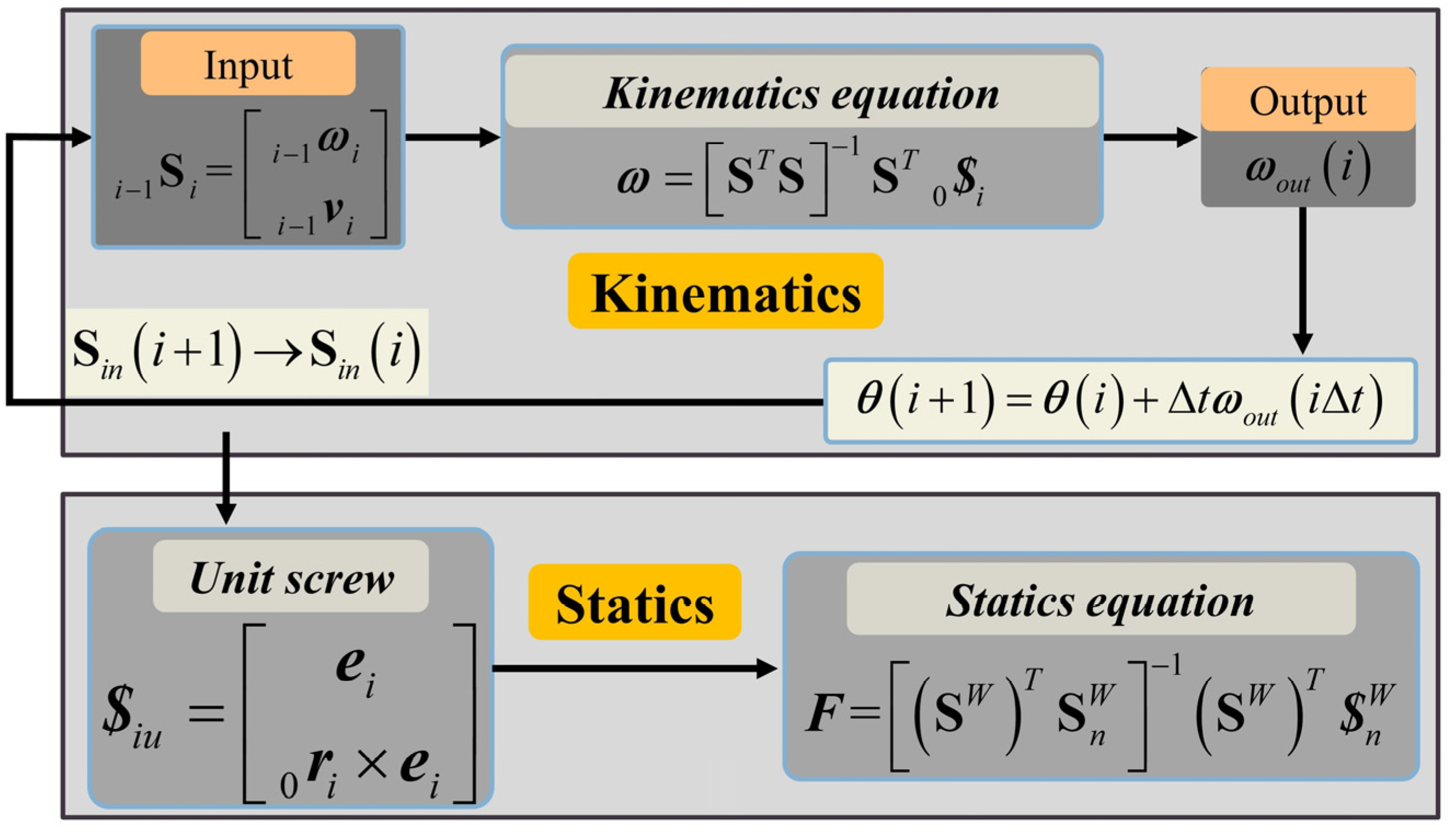
This paper proposes a kinematics and statics analysis method to analyze a Gough–Stewart platform in screw coordinates. Through defining the velocity screw, the relative angular and linear velocities of a point in a single rigid body can be combined into a dual vector with six components. The velocities of all joints can be derived in one direct step through the velocity screw equation. Then, the displacements and accelerations can be carried out separately through a first-order numerical integration and a first-order numerical differential interpolation, individually and simultaneously. Therefore, compared with the conventional modeling methods using displacements as global variables, the second-order numerical interpolation can be avoided in the proposed method in this paper, which eliminates complex algebraic manipulation and leads to more stable and accurate results. The velocity screw equation could be established to calculate the absolute position and absolute posture of all the joints and any point in a single rigid body. Through defining the force screw, both constraint forces and constraint torque at all joints could be expressed in screw form. Both forces and torques are considered in the equilibrium of a rigid body, and the force screw equation is established to express the resultant action of a force system in an absolute coordinate system. The unit screw matrix obtained in kinematic analysis can be directly applied in static analysis, which results in a compacter program structure. Then, the force screw equation using the unit screw matrix allows for a direct calculation of all constraint forces and torques at each joint.

The main contributions of this paper are summarized as follows:

(1)

Kinematics and statics modeling are unified via expressing parameters in screw coordinates. The kinematic parameters in screw form can be directly used in static equilibrium equations established using force screws.

(2)

Through combining kinematics and statics analysis, the forces and moments acting on each element of a mechanism in different configurations can be computed systematically.

(3)

The method proposed in this paper is highly universal and can be applied to the kinematics and statics analysis of variable mechanisms, and the validity of the method is verified via the kinematics and statics analysis of the Gough–Stewart platform.

Compared with the conventional static analysis method, using the velocity screw and the force screw might eliminate complex algebraic manipulation and allow for the direct calculation of the six constraint variables for all joints. This method can also be applied to other planar and spatial complex mechanisms and manipulators.

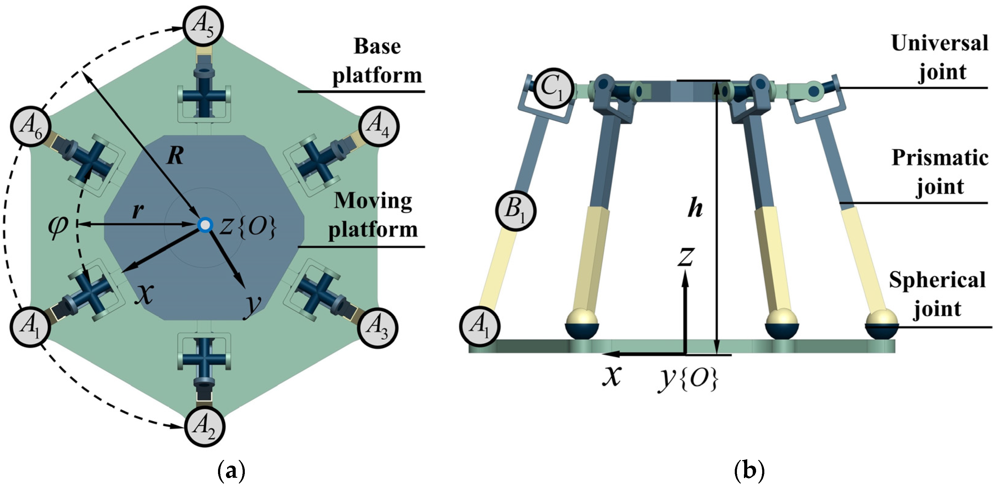
In this paper, the contents are arranged as follows: Section 2 introduces the geometry of the Gough–Stewart parallel mechanism. Section 3 describes the kinematic modeling method in screw form for multi-rigid-body systems and the kinematic modeling of the Gough–Stewart platform. Section 4 introduces the static modeling method using force screws and the unified kinematic and static modeling approach. The method is demonstrated through static modeling of the Gough–Stewart platform. In Section 5, the motion of the moving platform and the external loads are given, and the numerical simulation to perform the effectiveness of the modeling method is carried out. And finally, Section 6 concludes the paper.

2. Geometry of a Gough–Stewart Platform

The Gough–Stewart platform is composed of a moving platform and a base platform, and they are connected by six identical scalable kinematic chains. Every kinematic chain consists of one spherical pair (S), one universal pair (U), and one prismatic pair (P) as the actuated joint. In this paper, six universal pairs are assembled on the moving platform, and six spherical pairs are connected on the base platform. Six kinematic subchains are distributed uniformly around the $z\text{-}$axis shown in Figure 1. The origin of the absolute coordinate system is set at the geometric center of the base platform, the $z$-axis is perpendicular to the base platform and points to moving platform, the $x$-axis is superposed with $O{A}_1$, and the $y$-axis is obtained using the right-hand rule. Suppose the radius of the base platform is $R$, and the radius of the moving platform is $r$.

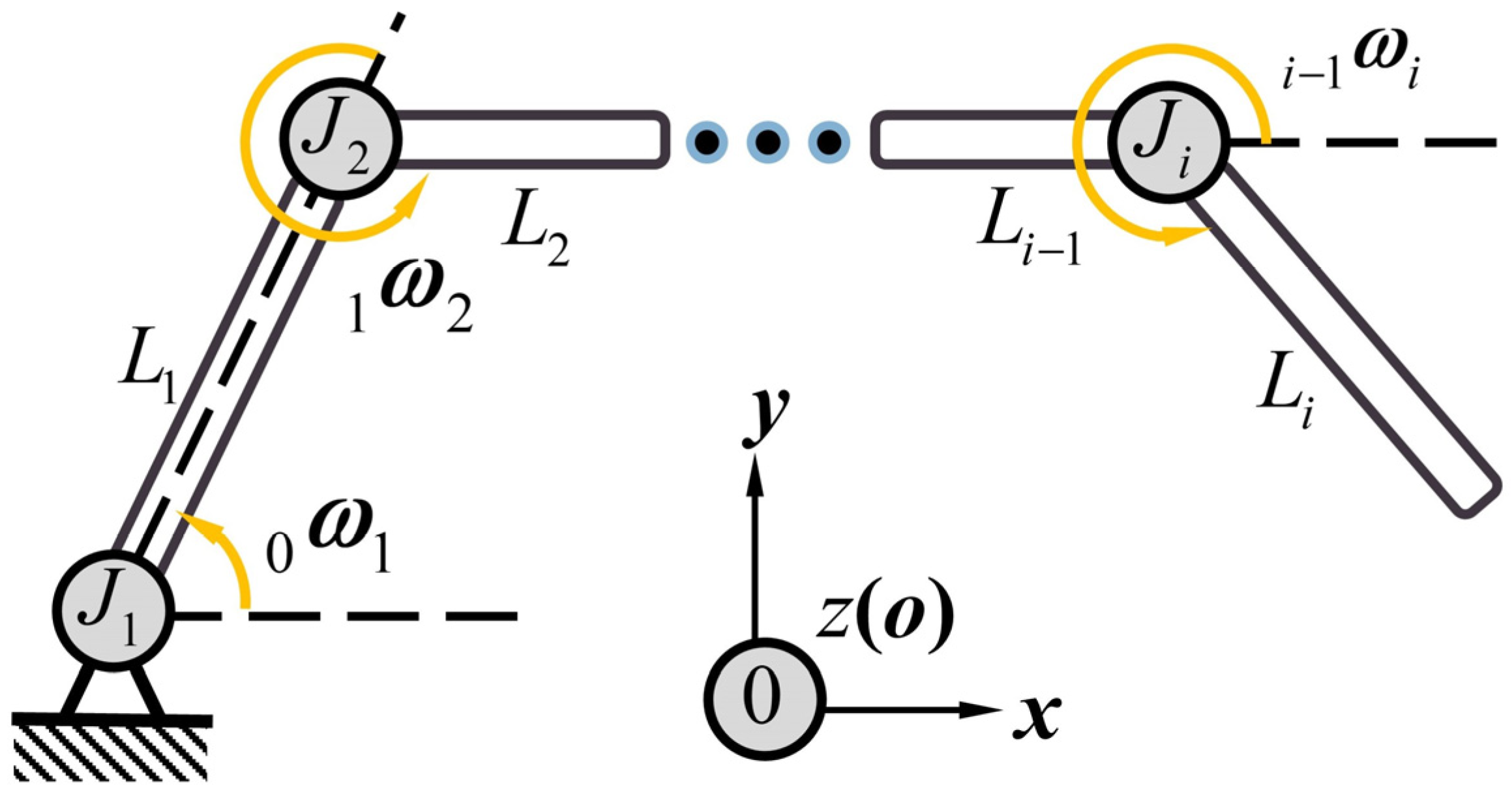
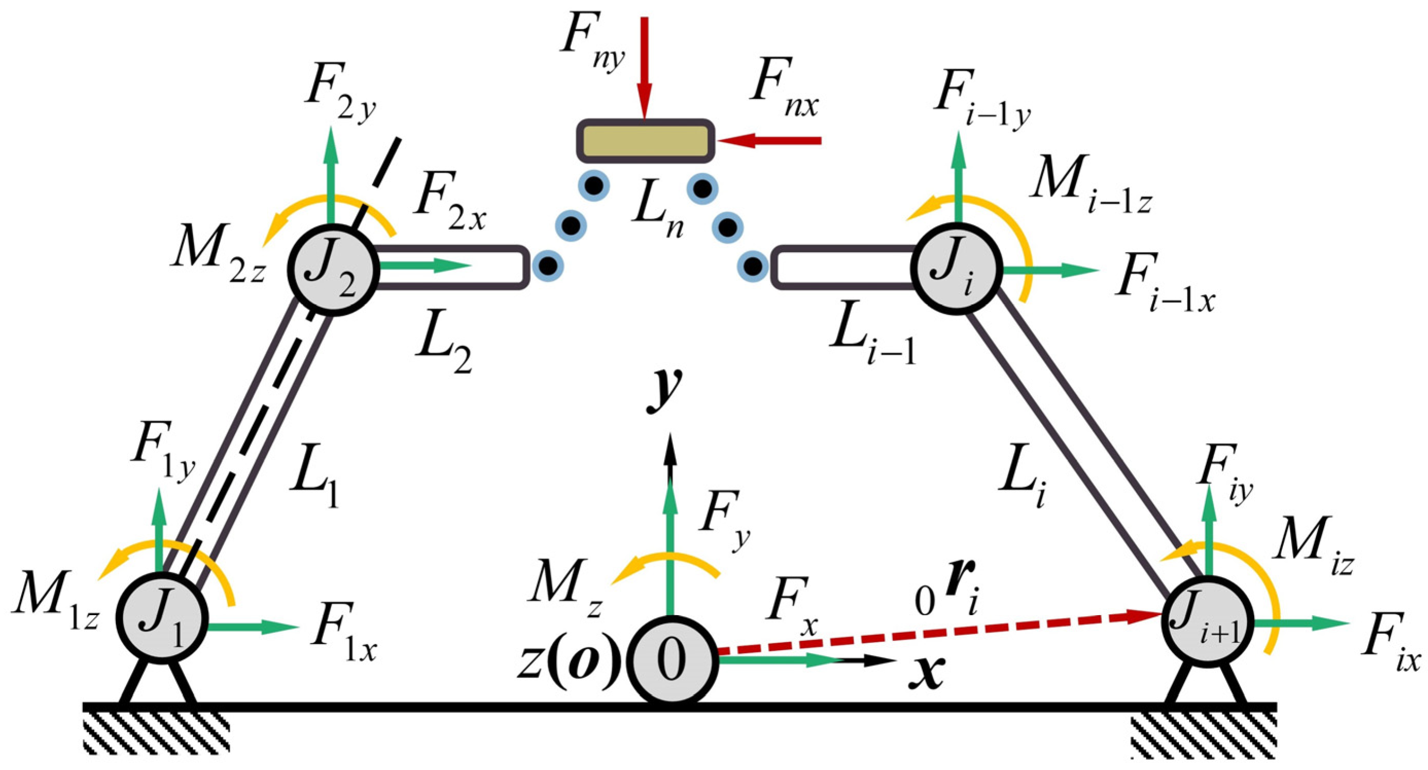
3. Kinematics of a Multi-Rigid System

As shown in Figure 2, suppose there are two single rigid linkages $L_{i-1}$ and $L_i$, which are connected by joint $J_i$ in an open kinematic chain.

The motion of a linkage can be described and determined according to the relative angular velocity and relative linear velocity. The relative angular velocity ${}_0\mathit{\omega }_1$ and relative linear velocity ${}_0\mathit{v}_1$ of link $L_1$ are two three-dimensional vectors, and both of them could be defined as a dual vector to form the velocity screw [27]:

$${}_0\mathsf{\$}_1=\left[\begin{array}{c}{}_0\mathit{\omega }_1\\ {}_0\mathit{v}_1\end{array}\right]$$

(1)

where ${}_0\mathit{\omega }_1$ is relative angular velocity from joint $J_1$ to the absolute coordinate 0, and ${}_0\mathit{v}_1$ is the relative linear velocity from joint $J_1$ to the coordinate origin 0.

The three-dimensional vector ${}_0\mathit{v}_1$ in Equation (1) can be expressed as ${}_0\mathit{v}_1={}_0\mathit{r}_1\times {}_0\mathit{\omega }_1$, where ${}_0\mathit{r}_1$ is the position vector of joint with respect to the origin of the absolute coordinate system.

Suppose $‖{\mathit{e}}_1‖=1$. Equation (1) can be rewritten as:

$${}_0\mathsf{\$}_1={}_0\omega _1\left[\begin{array}{c}{\mathit{e}}_1\\ {}_0\mathit{r}_1\times {\mathit{e}}_1\end{array}\right]$$

(2)

where ${\mathit{e}}_1$ is the unit direction vector of joint $J_1$, and ${}_0\omega _1$ is the amplitude of the relative angular velocity of joint $J_1$. Let

$${\mathsf{\$}}_{1u}=\left[\begin{array}{c}{\mathit{e}}_1\\ {}_0\mathit{r}_1\times {\mathit{e}}_1\end{array}\right]$$

(3)

where ${\mathsf{\$}}_{1u}$ is the unit velocity screw of joint $J_1$ [28].

Substituting Equation (3) into Equation (2) yields:

$${}_0\mathsf{\$}_1={}_0\omega _1{\mathsf{\$}}_{1u}$$

(4)

Within the unit velocity screw, the first three-dimensional vector presents the posture of the rotational motion, and the last three-dimensional vector contains the position parameters of the rotational motion.

3.1. Kinematics of an Open Kinematic Chain

For an open serial kinematic chain, based on the linear combination, the angular velocity and linear velocity of the terminal joint $J_i$ can be expressed as follows:

$$\left\{\begin{array}{l}{}_0\mathit{\omega }_i={}_0\mathit{\omega }_1+{}_1\mathit{\omega }_2+{}_2\mathit{\omega }_3+\cdots +{}_{i-2}\mathit{\omega }_{i-1}+{}_{i-1}\mathit{\omega }_i\\ {}_0\mathit{v}_i={}_0\mathit{v}_1+{}_1\mathit{v}_2+{}_2\mathit{v}_3+\cdots +{}_{i-2}\mathit{v}_{i-1}+{}_{i-1}\mathit{v}_i\end{array}\right.$$

(5)

where ${}_0\mathit{\omega }_i$ is the absolute angular velocity of the end joint $J_i$ with respect to the absolute coordinate system, and ${}_0\mathit{v}_i$ is the absolute linear velocity of the end joint $J_i$ with respect to the absolute coordinate frame.

With the definition of velocity screw in Equations (4) and (5), the forward kinematics of an open kinematics chain would be obtained such that

$${}_0\mathsf{\$}_i={\displaystyle \sum _{i=1}^n{}_{i-1}\mathsf{\$}_i}=\mathbf{S}\mathit{\omega }$$

(6)

where

$$\mathbf{S}=\left[\begin{array}{cccc}{\mathsf{\$}}_{1u}& {\mathsf{\$}}_{2u}& \cdots & {\mathsf{\$}}_{iu}\end{array}\right]$$

(7)

which presents the unit screw matrix of the serial linkage and

$$\mathit{\omega }={\left[\begin{array}{cccc}{}_0\omega _1& {}_1\omega _2& \cdots & {}_{i-1}\omega _i\end{array}\right]}^T$$

(8)

with $\mathit{\omega }$ representing the angular velocity vector, which contains all the velocity information of all joints in the kinematic chain.

With Equation (6), if the kinematics of the end link $J_i$ is given, the inverse kinematics of the open kinematic chain could be derived through:

$${\mathbf{S}}^T\mathbf{S}\mathit{\omega }={\mathbf{S}}^T{}_0\mathsf{\$}_i$$

(9)

When $\left|{\mathbf{S}}^T\mathbf{S}\right|=0$, the kinematic chain is a redundantly actuated mechanism, or it is in a singular configuration. Otherwise, the inverse kinematics of an open serial chain can be solved from Equation (9):

$$\mathit{\omega }={\left[{\mathbf{S}}^T\mathbf{S}\right]}^{-1}{\mathbf{S}}^T{}_0\mathsf{\$}_i$$

(10)

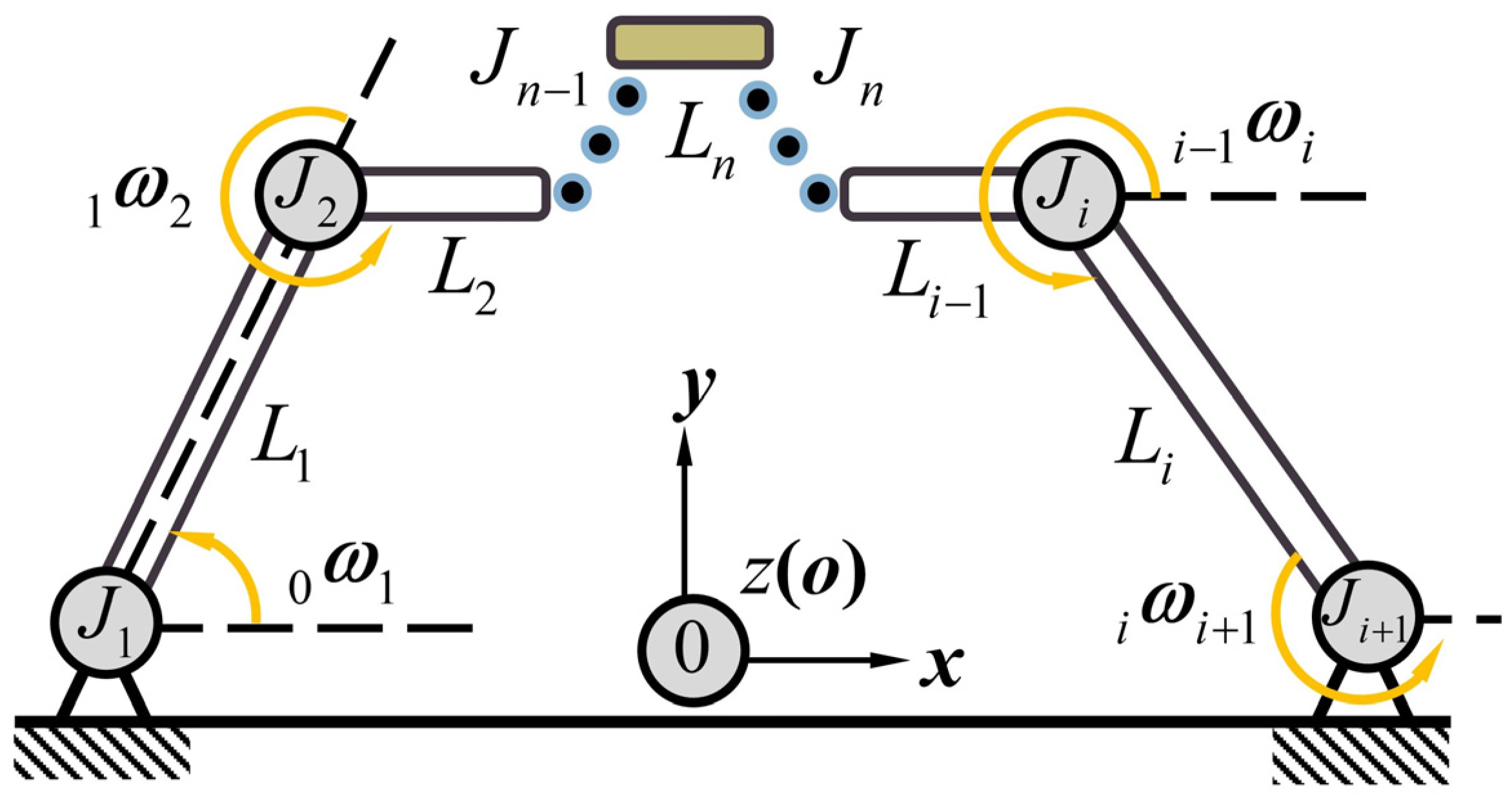
3.2. Kinematics of a Closed Kinematic Chain

A single closed kinematic chain is illustrated in Figure 3. Based on the linear combination, the kinematics of the end joint $J_{i+1}$ can be expressed as:

$$\left\{\begin{array}{l}{}_0\mathit{\omega }_{i+1}={}_0\mathit{\omega }_1+{}_1\mathit{\omega }_2+{}_2\mathit{\omega }_3+\cdots +{}_{i-2}\mathit{\omega }_{i-1}+{}_{i-1}\mathit{\omega }_i+{}_i\mathit{\omega }_{i+1}\\ {}_0\mathit{v}_{i+1}={}_0\mathit{v}_1+{}_1\mathit{v}_2+{}_2\mathit{v}_3+\cdots +{}_{i-2}\mathit{v}_{i-1}+{}_{i-1}\mathit{v}_i+{}_i\mathit{v}_{i+1}\end{array}\right.$$

(11)

The absolute angular velocity and absolute linear velocity of joint $J_{i+1}$ on the expanded rigid body of link $L_i$ that is superimposed with the origin of the coordinate system are 0. Therefore, Equation (11) can be rewritten as:

$$\left\{\begin{array}{l}0={}_0\mathit{\omega }_1+{}_1\mathit{\omega }_2+{}_2\mathit{\omega }_3+\cdots +{}_{i-2}\mathit{\omega }_{i-1}+{}_{i-1}\mathit{\omega }_i+{}_i\mathit{\omega }_{i+1}\\ 0={}_0\mathit{v}_1+{}_1\mathit{v}_2+{}_2\mathit{v}_3+\cdots +{}_{i-2}\mathit{v}_{i-1}+{}_{i-1}\mathit{v}_i+{}_i\mathit{v}_{i+1}\end{array}\right.$$

(12)

With Equations (6) and (12), the forward kinematics of a single closed kinematic chain can be derived as:

$${}_0\mathsf{\$}_{i+1}={\displaystyle \sum _{i=0}^n{}_i\mathsf{\$}_{i+1}}=0$$

(13)

When the kinematics of any link $L_n$ in the closed serial kinematic chain shown in Figure 3 are given in the absolute coordinate system, that is to say, the screw matrix ${}_0\mathsf{\$}_n$ of link $L_n$ is known, the inverse kinematics of the single closed kinematic chain could be solved based on Equation (6):

$$\begin{array}{l}{}_0\mathsf{\$}_n={}_0\mathsf{\$}_1+{}_1\mathsf{\$}_2+\cdots +{}_{n-2}\mathsf{\$}_{n-1}+{}_{n-1}\mathsf{\$}_n\\ -{}_0\mathsf{\$}_n={}_n\mathsf{\$}_{n+1}+{}_{n+1}\mathsf{\$}_{n+2}+\cdots +{}_{i-2}\mathsf{\$}_{i-1}+{}_{i-1}\mathsf{\$}_i\end{array}$$

(14)

where only ${}_0\mathsf{\$}_n$ is known.

When the kinematics of all joint except the link $L_n$ are prescribed, the forward kinematics of the single closed kinematic chain could be obtained based on Equation (6) through

$$\begin{array}{l}{}_{n-1}\mathsf{\$}_n={}_0\mathsf{\$}_1+{}_1\mathsf{\$}_2+\cdots +{}_{n-2}\mathsf{\$}_{n-1}+{}_n\mathsf{\$}_{n+1}+\cdots +{}_{i-2}\mathsf{\$}_{i-1}+{}_{i-1}\mathsf{\$}_i\\ {}_0\mathsf{\$}_n={}_0\mathsf{\$}_1+{}_1\mathsf{\$}_2+\cdots +{}_{n-2}\mathsf{\$}_{n-1}+{}_{n-1}\mathsf{\$}_n\end{array}$$

(15)

where ${}_{n-1}\mathsf{\$}_n$ is the relative velocity screw, and ${}_0\mathsf{\$}_n$ is the absolute velocity screw.

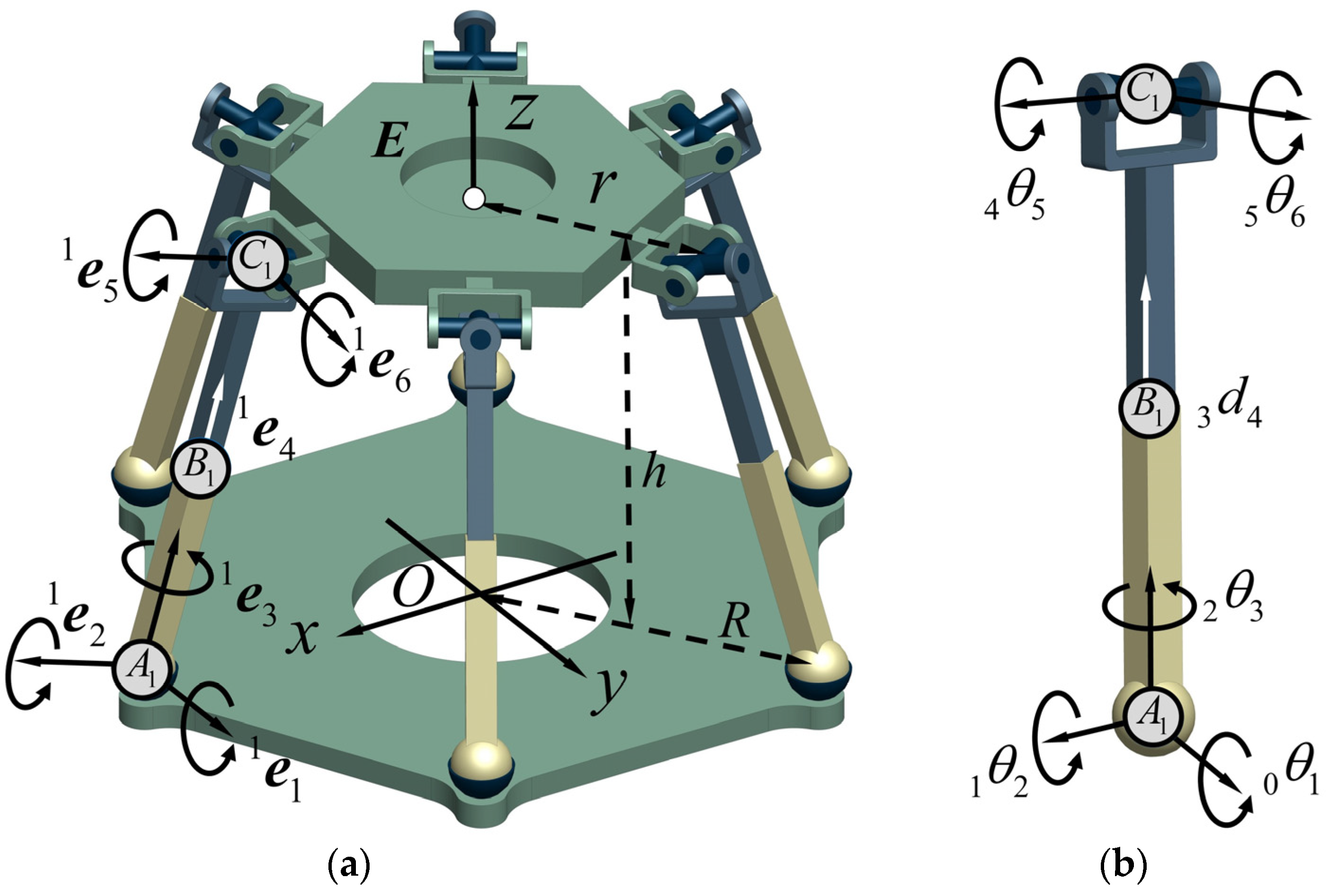
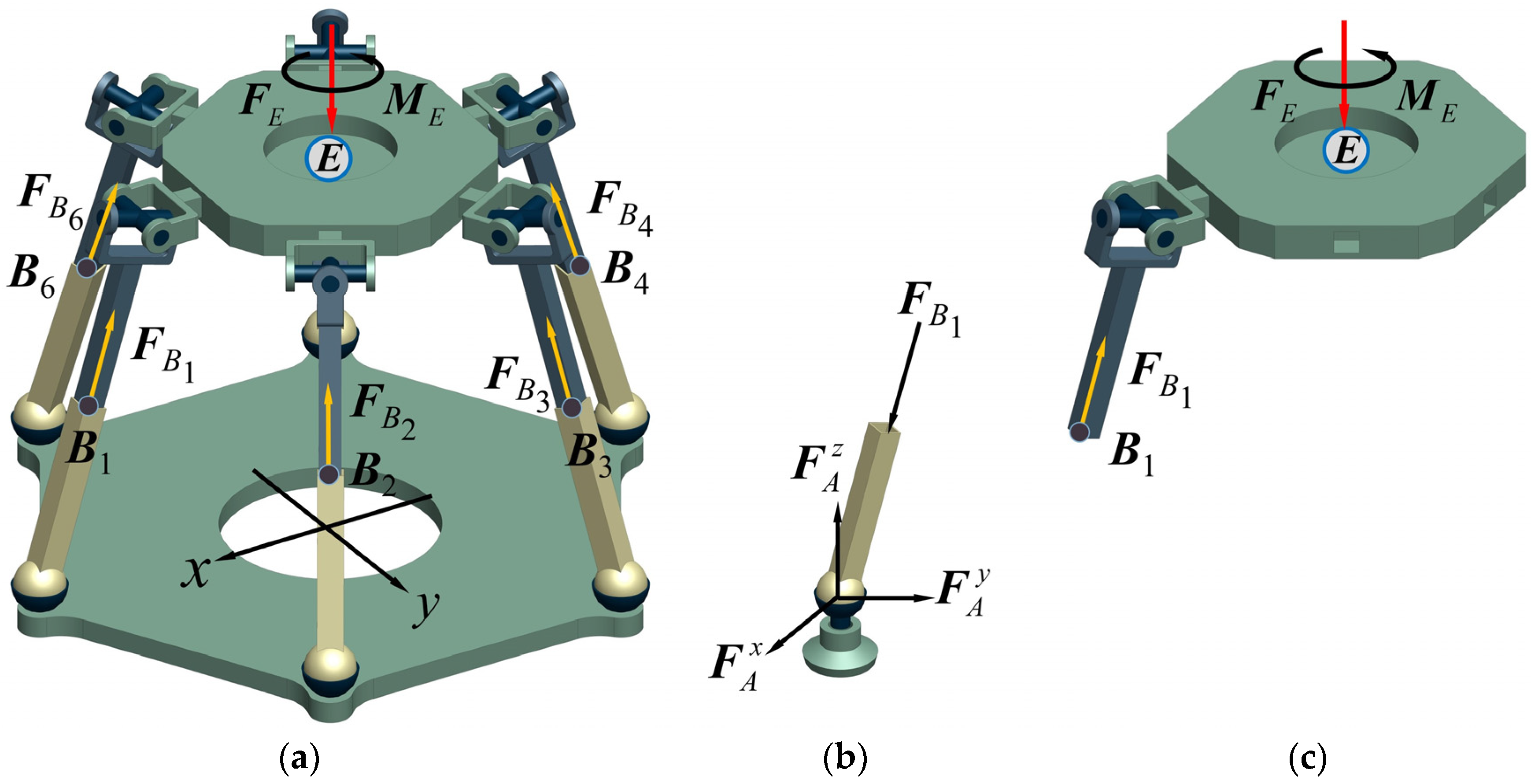
3.3. Kinematics of Gough–Stewart Platform

In this section, the inverse kinematics of the Gough–Stewart platform are computed. As depicted in Figure 4, the inverse kinematic equation of the Gough–Stewart platform can be established as:

$${\mathsf{\$}}_E={\mathbf{S}}_{ABC,i}{\mathit{\omega }}_{ABC,i},\left(i=1,2,\cdots ,6\right)$$

(16)

where $i$ represents the $i$-th subchain of the Gough–Stewart platform.

For the first kinematic chain $L_{ABC,1}$, the unit velocity screw equation of the moving platform can be expressed as:

$${\mathsf{\$}}_E={\mathbf{S}}_{ABC,1}{\mathit{\omega }}_{ABC,1}$$

(17)

where ${\mathbf{S}}_{ABC,1}=\left[\begin{array}{cccccc}{}_0\mathsf{\$}_{1,1}& {}_1\mathsf{\$}_{2,1}& {}_2\mathsf{\$}_{3,1}& {}_3\mathsf{\$}_{4,1}& {}_4\mathsf{\$}_{5,1}& {}_5\mathsf{\$}_{6,1}\end{array}\right]$ is the unit screw matrix of the first kinematic subchain, with velocity screws ${}_0\mathsf{\$}_{1,1}=\left[\begin{array}{c}{\mathit{e}}_{1,1}\\ {}_0\mathit{r}_{A_1}\times {\mathit{e}}_{1,1}\end{array}\right]$, ${}_1\mathsf{\$}_{2,1}=\left[\begin{array}{c}{\mathit{e}}_{2,1}\\ {}_0\mathit{r}_{A_1}\times {\mathit{e}}_{2,1}\end{array}\right]$, ${}_2\mathsf{\$}_{3,1}=\left[\begin{array}{c}{\mathit{e}}_{3,1}\\ {}_0\mathit{r}_{A_1}\times {\mathit{e}}_{3,1}\end{array}\right]$, ${}_3\mathsf{\$}_{4,1}=\left[\begin{array}{c}0\\ {\mathit{e}}_{4,1}\end{array}\right]$, ${}_4\mathsf{\$}_{5,1}=\left[\begin{array}{c}{\mathit{e}}_{5,1}\\ {}_0\mathit{r}_{C_1}\times {\mathit{e}}_{5,1}\end{array}\right]$, ${}_5\mathsf{\$}_{6,1}=\left[\begin{array}{c}{\mathit{e}}_{6,1}\\ {}_0\mathit{r}_{C_1}\times {\mathit{e}}_{6,1}\end{array}\right]$, and ${\mathit{\omega }}_{ABC,1}={\left[\begin{array}{cccccc}{}_0\omega _{1,1}& {}_1\omega _{2,1}& {}_2\omega _{3,1}& {}_3\mathit{v}_{4,1}& {}_4\omega _{5,1}& {}_5\omega _{6,1}\end{array}\right]}^T$.

Equation (17) is the velocity screw equation of the kinematic chain $L_{ABC,1}$ which can be applied to solve the relative angular velocities and relative linear velocities. Therefore, Equation (17) could be rewritten as:

$${\mathbf{S}}_{ABC,1}=\left[\begin{array}{cccccc}{\mathit{e}}_{1,1}& {\mathit{e}}_{2,1}& {\mathit{e}}_{3,1}& {\mathsf{0}}_{3\times 1}& {\mathit{e}}_{5,1}& {\mathit{e}}_{6,1}\\ {}_0\mathit{r}_{A_1}\times {\mathit{e}}_{1,1}& {}_0\mathit{r}_{A_1}\times {\mathit{e}}_{2,1}& {}_0\mathit{r}_{A_1}\times {\mathit{e}}_{3,1}& {\mathit{e}}_{4,1}& {}_0\mathit{r}_{C_1}\times {\mathit{e}}_{5,1}& {}_0\mathit{r}_{C_1}\times {\mathit{e}}_{6,1}\end{array}\right]$$

(18)

In order to obtain the unit screws in Equation (18), the rotation transformation matrix is applied to express ${\mathit{e}}_{j,i},{\mathit{r}}_{j,i}$ of each joint in the local coordinate system; $i$ represents the $i$-th chain and $j$ represents the $j$-th joint in this chain.

$$\left\{\begin{array}{l}{\mathit{e}}_{j,i}={\mathbf{R}}_{Z,i}\left({\displaystyle \mathsf{\prod }_{j=2}{\mathbf{R}}_{j,i}}\right){\mathit{e}}_{j,i}\left(0\right)\\ {\mathit{r}}_{j,i}={\mathbf{R}}_{Z,i}\left({}_0\mathit{r}_{A,i}\left(0\right)+{\mathbf{R}}_2{\mathbf{R}}_3{\mathbf{R}}_5{\mathit{r}}_{\mathit{r}od}^j\right)\end{array}\right.,\left(i=1,2,\cdots ,6;j=1,2,\cdots ,6\right)$$

(19)

where ${\mathbf{R}}_{Z,i}$ is the rotation transformation matrix around the $z$-axis, and it can be expressed as ${\mathbf{R}}_{Z,i}={\mathbf{R}}_z\left(\left(i-1\right){30}^{\circ }\right)$. ${\mathbf{R}}_j$ is the rotation transformation matrix from link $L_i$ to link $L_{i-1}$; when it rotates around the $x$-axis, ${\mathbf{R}}_j={\mathbf{R}}_x\left({}_{j-1}\theta _{j,i}\right)$; when it rotates around $y$-axis, ${\mathbf{R}}_j={\mathbf{R}}_y\left({}_{j-1}\theta _{j,i}\right)$; and when it rotates around $z$-axis, ${\mathbf{R}}_j={\mathbf{R}}_z\left({}_{j-1}\theta _{j,i}\right)$.

Suppose the velocity screw of the moving platform is given; the relative angular velocity of each kinematic chain $L_{ABC,i},\left(i=1,2,\cdots ,6\right)$ could be calculated using Equation (17).

$${\mathit{\omega }}_{ABC,i}={\left[{\mathbf{S}}_{ABC,i}^{\mathit{T}}{\mathbf{S}}_{ABC,i}\right]}^{-1}{\mathbf{S}}_{ABC,i}^{\mathit{T}}{\mathsf{\$}}_E,\left(i=1,2,\cdots ,6\right)$$

(20)

where ${\mathsf{\$}}_E=\left[\begin{array}{c}{}_0\mathit{\omega }_E\\ {}_0\mathit{v}_E+{}_0\mathit{r}_E\times {}_0\mathit{\omega }_E\end{array}\right]$, ${}_0\mathit{\omega }_E$ is the absolute angular velocity of the moving platform and ${}_0\mathit{v}_E$ is the absolute linear velocity of the moving platform with respect to the absolute coordinate frame.

4. Statics of the Gough–Stewart Platform in Plücker Coordinate

4.1. Statics of a Series Kinematic Chain

The equilibrium of an ideal object without considering its size is stated by Newton’s first law. Force and couple are two basic physical quantities of statics. In reality, the parameters of forces and torques, such as magnitude and acting position, are taken into account in the equilibrium of a rigid body. We therefore discuss the action of forces and couples on a rigid body together.

Suppose that there is an external force ${\mathit{F}}_n$ exerted on rigid link $L_n$ as shown in Figure 5. Therefore, a force ${\mathit{F}}_i$ and a torque ${\mathit{M}}_i$ should be applied to joint $J_i,(i=1,2,\cdots )$ to maintain the equilibrium of the chain.

Associating the force ${\mathit{F}}_i$ with the couple of ${}_0\mathit{r}_i\times {\mathit{F}}_i$, where ${}_0\mathit{r}_i$ is the position vector from the origin to joint $J_i$, the force screw can be expressed as:

$${\mathsf{\$}}_i^W=\left[\begin{array}{c}{\mathit{F}}_i\\ {}_0\mathit{r}_i\times {\mathit{F}}_i\end{array}\right]=\left[\begin{array}{c}{\mathit{F}}_i\\ {\mathit{M}}_i\end{array}\right]$$

(21)

In Equation (21), ${\mathit{F}}_i$ is called the force vector of the force screw and ${\mathit{M}}_i={}_0\mathit{r}_i\times {\mathit{F}}_i$ represents the moment of the force about the origin.

Suppose ${\mathit{e}}_i$ presents the unit direction vector of force ${\mathit{F}}_i$, namely $‖{\mathit{e}}_i‖=1$, where $‖\cdot ‖$ indicates the norm of vector ‘$\cdot$’. Equation (21) can be rewritten as:

$${\mathsf{\$}}_i^W={\mathit{F}}_i{\mathsf{\$}}_{iu}$$

(22)

with ${\mathsf{\$}}_{iu}=\left[\begin{array}{c}{\mathit{e}}_i\\ {}_0\mathit{r}_i\times {\mathit{e}}_i\end{array}\right]$.

The equilibrium condition of the rigid object, whose external loads are all expressed in screw coordinates, should be that the resultant force screw must be zero:

$${\displaystyle \sum _{i=1}^n{\mathsf{\$}}_i^W}=0$$

(23)

When there is an external load exerted on the mechanism, which can be expressed as ${\mathsf{\$}}_n^W$, Equation (23) is rewritten as:

$${\mathbf{S}}^W\mathit{F}={\mathsf{\$}}_n^W$$

(24)

where ${\mathbf{S}}^W=\left[\begin{array}{cccc}{\mathsf{\$}}_{1u}& {\mathsf{\$}}_{2u}& \cdots & {\mathsf{\$}}_{iu}\end{array}\right]$ is the unit force screw matrix composed of unit force screws of each joint, and the force vector $\mathit{F}={\left[\begin{array}{cccc}{F}_1& F_2& \cdots & F_i\end{array}\right]}^T$ contains all force information of each joint. Therefore, the inverse statics of each joint $J_i$ could be carried out through Equation (24):

$${\left({\mathbf{S}}^W\right)}^T{\mathbf{S}}^W\mathit{F}={\left({\mathbf{S}}^W\right)}^T{\mathsf{\$}}_n^W$$

(25)

When $\left|{\left({\mathbf{S}}^W\right)}^T{\mathbf{S}}_n^W\right|=0$, the kinematic chain is a redundantly actuated mechanism, or it is in a singular configuration. Otherwise, Equation (25) could be further derived as:

$$\mathit{F}={\left[{\left({\mathbf{S}}^W\right)}^T{\mathbf{S}}_n^W\right]}^{-1}{\left({\mathbf{S}}^W\right)}^T{\mathsf{\$}}_n^W$$

(26)

Based on the definition of velocity screw and force screw, the kinematic and static modeling could be associated with each other through unit screws. Through Equations (6), (7) and (10), expressed in Section 3, the unit screw ${\mathsf{\$}}_{iu}$ of each joint in the absolute coordinate system, which consists of position ${}_0\mathit{r}_i$ and posture ${\mathit{e}}_i$, could be obtained via an iterative procedure. And the solved kinematic parameters, which are expressed in screw form, can be directly employed in establishing the static equations based on Equation (26). The relationship and unified procedure of the kinematic and static modeling of a kinematic chain are given in Figure 6.

4.2. Statics of the Gough–Stewart Platform

Figure 7 illustrates a Gough–Stewart platform, which is a representative multi-loop spatial mechanism. For the sake of generality, suppose that there are three external forces, ${\mathit{F}}_E^x$, ${\mathit{F}}_E^y$ and ${\mathit{F}}_E^z$, and three external torques, ${\mathit{T}}_E^x$, ${\mathit{T}}_E^y$ and ${\mathit{T}}_E^z$, exerted on the moving platform $E$.

In the absolute coordinate system shown in Figure 7a, the force screws of the external loads can be expressed as:

$${\mathsf{\$}}_E^W={\left[\begin{array}{cccccc}{F}_E^x& F_E^y& F_E^z& M_E^x& M_E^y& M_E^z\end{array}\right]}^T$$

(27)

The force screws of each prismatic joint $B_i(i=1,2,\cdots ,6)$ can be expressed as:

$${\mathsf{\$}}_{F_{B_i}}=F_{B_i}\left[\begin{array}{c}{\mathit{e}}_{B_i}\\ {\mathit{r}}_{B_i}\times {\mathit{e}}_{B_i}\end{array}\right]$$

(28)

where ${\mathit{r}}_{B_i}$ is the absolute position vector of joint $B_i$, and ${\mathit{e}}_{B_i}$ presents its posture.

The moving platform would maintain stable under the action of external loads expressed by these force screws. Therefore, we obtain the following equations:

$${\mathbf{S}}^W{\mathit{F}}_{B_i}={\mathsf{\$}}_E^W$$

(29)

where ${\mathbf{S}}^W=\left[\begin{array}{cccccc}\begin{array}{c}{\mathit{e}}_{B_1}\\ {\mathit{r}}_{B_1}\times {\mathit{e}}_{B_1}\end{array}& \begin{array}{c}{\mathit{e}}_{B_2}\\ {\mathit{r}}_{B_2}\times {\mathit{e}}_{B_2}\end{array}& \begin{array}{c}{\mathit{e}}_{B_3}\\ {\mathit{r}}_{B_3}\times {\mathit{e}}_{B_3}\end{array}& \begin{array}{c}{\mathit{e}}_{B_4}\\ {\mathit{r}}_{B_4}\times {\mathit{e}}_{B_4}\end{array}& \begin{array}{c}{\mathit{e}}_{B_5}\\ {\mathit{r}}_{B_5}\times {\mathit{e}}_{B_5}\end{array}& \begin{array}{c}{\mathit{e}}_{B_6}\\ {\mathit{r}}_{B_6}\times {\mathit{e}}_{B_6}\end{array}\end{array}\right]$ is the unit force screw matrix and ${\mathit{F}}_{B_i}={\left[\begin{array}{cccccc}{F}_{B_1}& F_{B_2}& F_{B_3}& F_{B_4}& F_{B_5}& F_{B_6}\end{array}\right]}^T$ represents the force vector.

The mechanism is in singularity when it satisfies $\left|{\mathbf{S}}^W{\left({\mathbf{S}}^W\right)}^T\right|=0$. Otherwise, we could obtain the solution of ${\mathit{F}}_{B_i}$ through:

$${\mathit{F}}_{B_i}={\left[{\mathbf{S}}^W{\left({\mathbf{S}}^W\right)}^T\right]}^{-1}{\left({\mathbf{S}}^W\right)}^T{\mathsf{\$}}_E^W$$

(30)

Through Equation (30), the driven forces of each limb shown in Figure 7b,c can be computed. With projection equations, we immediately obtain:

$${\mathit{F}}_{B_i}=F_{B_i}{\mathit{e}}_i$$

(31)

Equation (31) provides the general equation of static equilibrium for a single rigid object, and also for a multi-rigid-body system. Force screws are particularly suitable for programming a computer for analyzing the statics of multi-body systems.

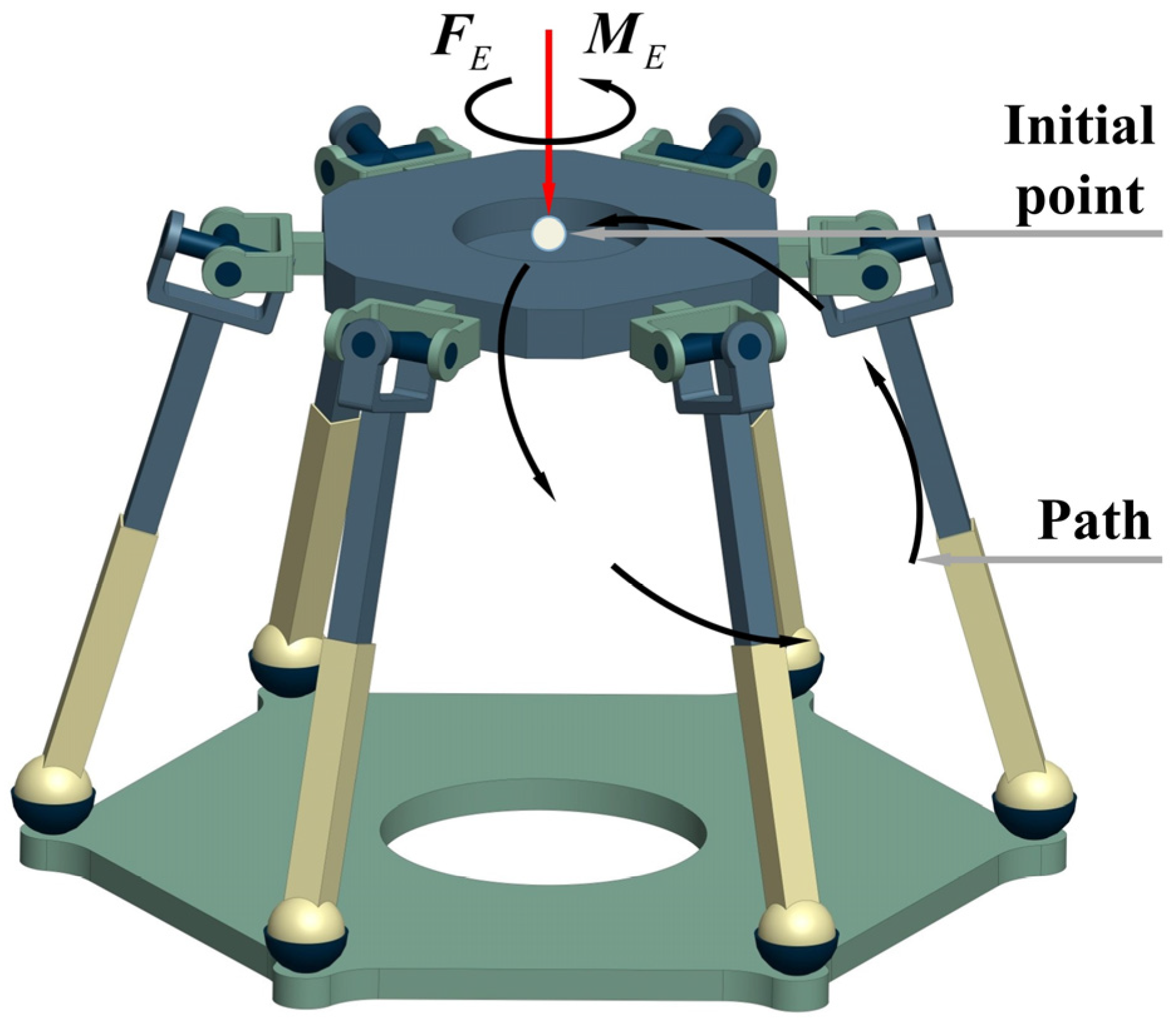
5. Numerical Experiment and Discussion

In order to verify the static modeling method of the Stewart platform, a trajectory of the moving platform is prescribed for the inverse kinematics, which is shown in Figure 8. The Gough–Stewart platform has six DoFs consisting of three translational motions and three rotational motions. Given a translational path of a circular trajectory for the moving platform, the parametric equations of the trajectory in the absolute coordinate system are expressed as:

$$\left\{\begin{array}{c}x\left(t\right)=-10\cos \left(t\right)\\ y\left(t\right)=-10\sin \left(t\right)\\ z\left(t\right)=20\cos \left(t\right)\end{array}\right.$$

(32)

where $x\left(t\right)$, $y\left(t\right)$, and $z\left(t\right)$ are the three motion variables of the center point on the moving platform at time $t$. From Equation (32), the unit velocity screw of the moving platform can be written as ${}_0\mathsf{\$}_{iu}={\left[\begin{array}{cccccc}0& 0& 1& 10\sin \left(n\Delta t\right)& 10\cos \left(n\Delta t\right)& 0\end{array}\right]}^{\mathit{T}}$, and the discrete conditions are shown in

Table 1. Discrete conditions of the simulation.

Discrete Condition	Parameters	Value
Total time of the path	$t\left(s\right)$	$10$
Interval of iteration	$\Delta t$	$0.001$
Steps of iteration	$k$	$10000$

. The kinematics analysis of the Gough–Stewart platform is performed through programming the introduced algorithm in MATLAB 2018a. These programs are executed on Windows 11 computers equipped with AMD Ryzen 7 6800HS with Radeon Graphics 3.20 GHz.

The displacement parameters of each joint are obtained through the numerical calculation method. Therefore, using the numerical calculation method introduces differences between the real solution of a practical problem and the approximate solution obtained via numerical calculation. In the iteration simulation, the errors could be minimized through optimizing the step length of the discrete conditions. There are no big differences between the results when the interval of iteration is smaller than 0.001, and it only brings high computation costs.

With the initial conditions of displacement ${\theta }_{j,i}^{}\left(0\right)$ illustrated in

Table 2. Initial configuration parameters of the Gough–Stewart platform.

${\theta }_{1,i}\left(0\right)\left(\mathrm{rad}\right)$	${\theta }_{2,i}\left(0\right)\left(\mathrm{rad}\right)$	${\theta }_{3,i}\left(0\right)\left(\mathrm{rad}\right)$	$d_{4,i}\left(0\right)\left(\mathrm{mm}\right)$	${\theta }_{5,i}\left(0\right)\left(\mathrm{rad}\right)$	${\theta }_{6,i}\left(0\right)\left(\mathrm{rad}\right)$
$\left\{{\theta }_{1,i}\right\}=\left\{-\frac{\pi }{6}\right\}$	$\left\{{\theta }_{2,i}\right\}=\left\{0\right\}$	$\left\{{\theta }_{3,i}\right\}=\left\{0\right\}$	$\left\{d_{4,i}\right\}=\left\{0\right\}$	$\left\{{\theta }_{5,i}\right\}=\left\{0\right\}$	$\left\{{\theta }_{6,i}\right\}=\left\{-\frac{\pi }{3}\right\}$

, the initial relative angular velocities ${\mathit{\omega }}_i\left(1\right)$ of the i-th kinematic chain could be derived using Equation (20).

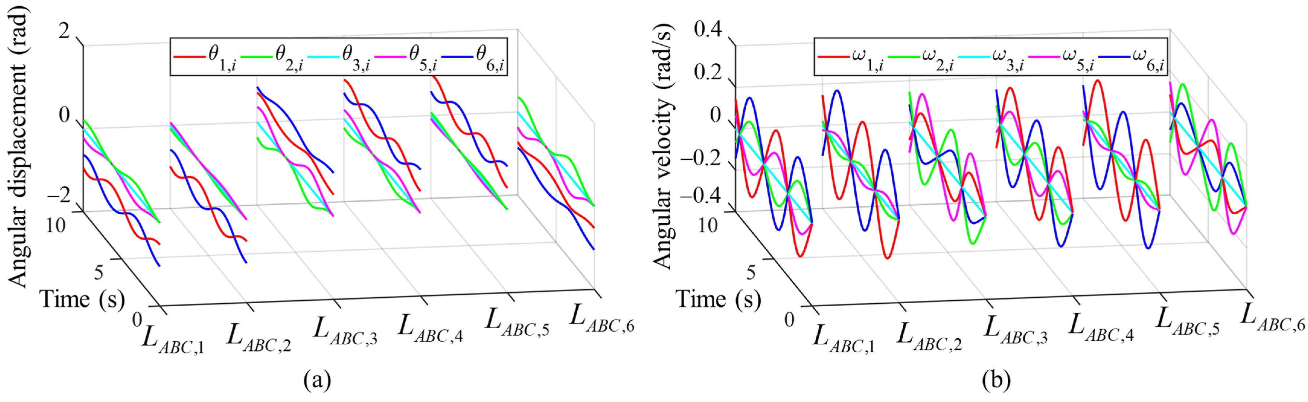
Figure 9 shows the angular displacements (Figure 9a) and angular velocities (Figure 9b) of each revolute joint in six kinematic chains.

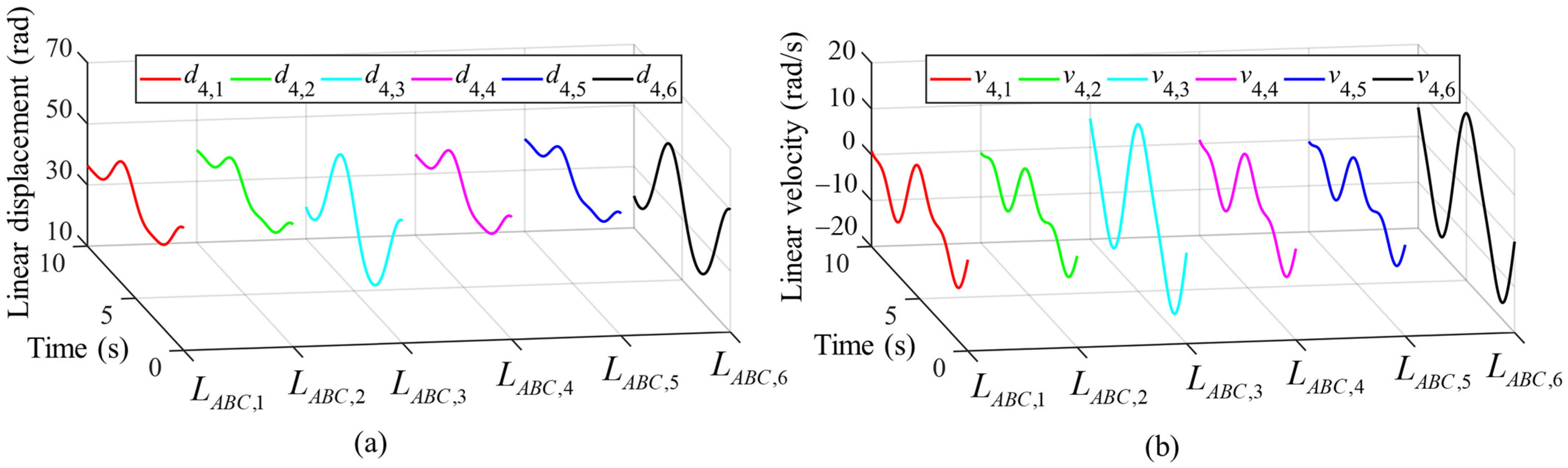
Figure 10 depicts the linear displacement (Figure 10a) and linear velocity (Figure 10b) of the linear pairs of each kinematic chain. All diagrams are plotted in MATLAB 2018a.

According to the inverse kinematics that are calculated in the above section, the kinematics of each joint in the absolute coordinate system could be calculated. Suppose there are an external force ${\mathit{F}}_E=\left[\begin{array}{ccc}0& 0& 10\end{array}\right]\left(kN\right)$ and a torque ${\mathit{M}}_E=\left[\begin{array}{ccc}0& 0& 10\end{array}\right]\left(kN\cdot m\right)$ exerted on the moving platform, which are shown in Figure 7 and Figure 8. And the force screw of the moving platform can be expressed in screw coordinates:

$$\left[\begin{array}{c}{\mathit{F}}_E\left(t\right)\\ {\mathit{M}}_E\left(t\right)\end{array}\right]={\left[\begin{array}{cccccc}0& 0& 10& 100\sin \left(k\Delta t\right)& -100\cos \left(k\Delta t\right)& -200\sin \left(k\Delta t\right)+10\end{array}\right]}^{\mathit{T}}$$

(33)

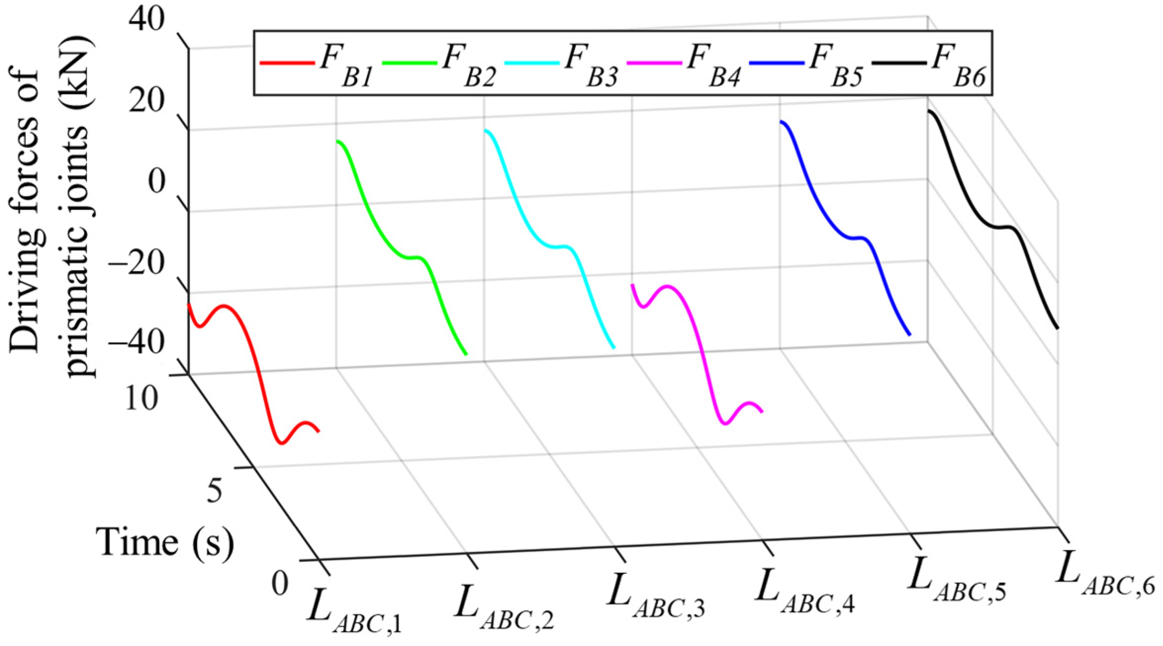
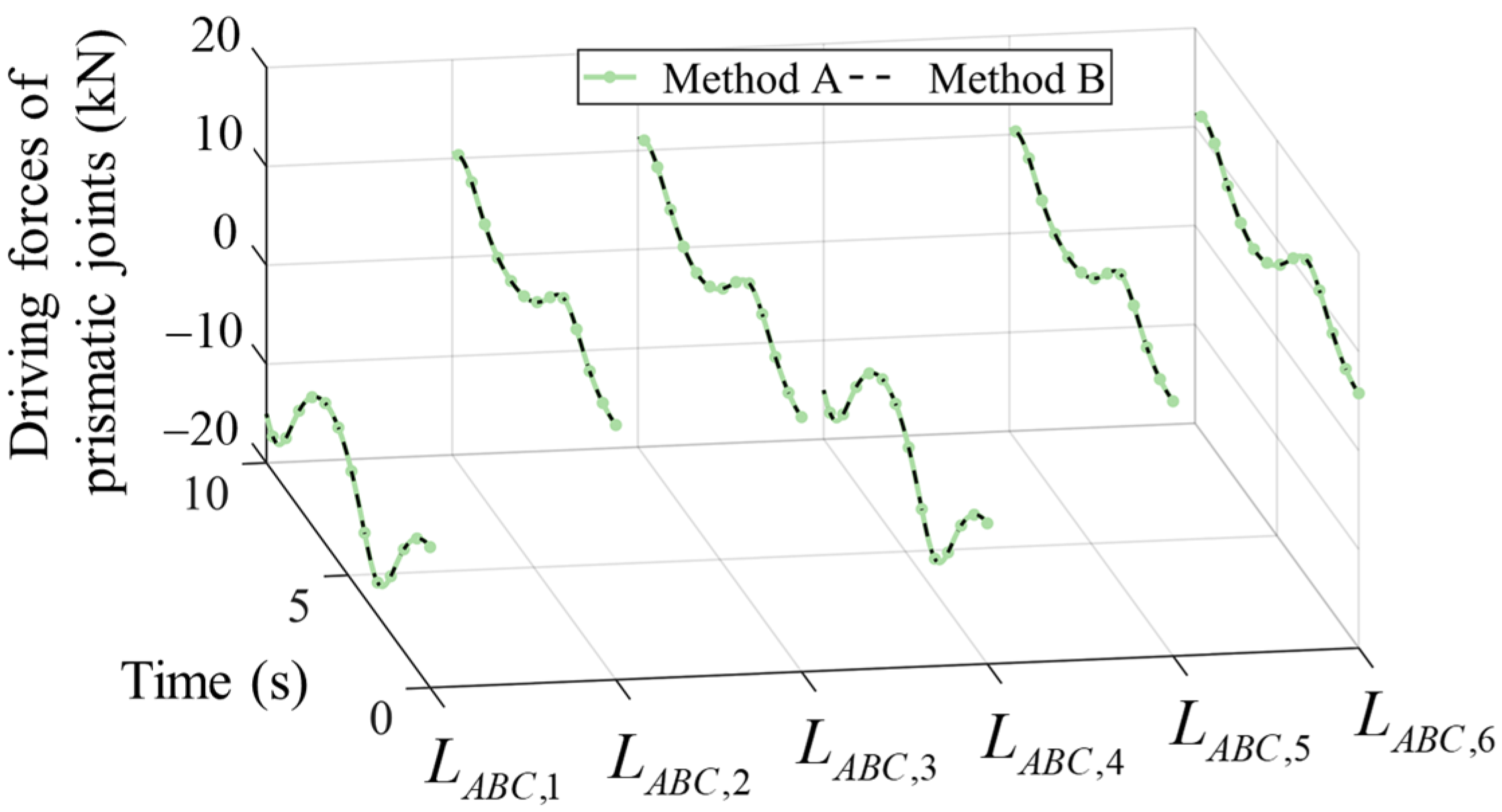
In this paper, the mass and inertia properties of the Gough–Stewart platform are ignored. Based on the structure parameters and the external forces and torques added to the moving platform, the driving forces ${\mathit{F}}_{B,i}$ to hold the equilibrium of the mechanism could be calculated through carrying out the proposed statics analysis, and the results are plotted in Figure 11. It is clear that the driving forces are adjusted to maintain equilibrium during the motion process. The simulation results in Figure 9, Figure 10 and Figure 11 show that no sudden changes in velocities or driving forces appeared and that the mechanism was never in singularity.

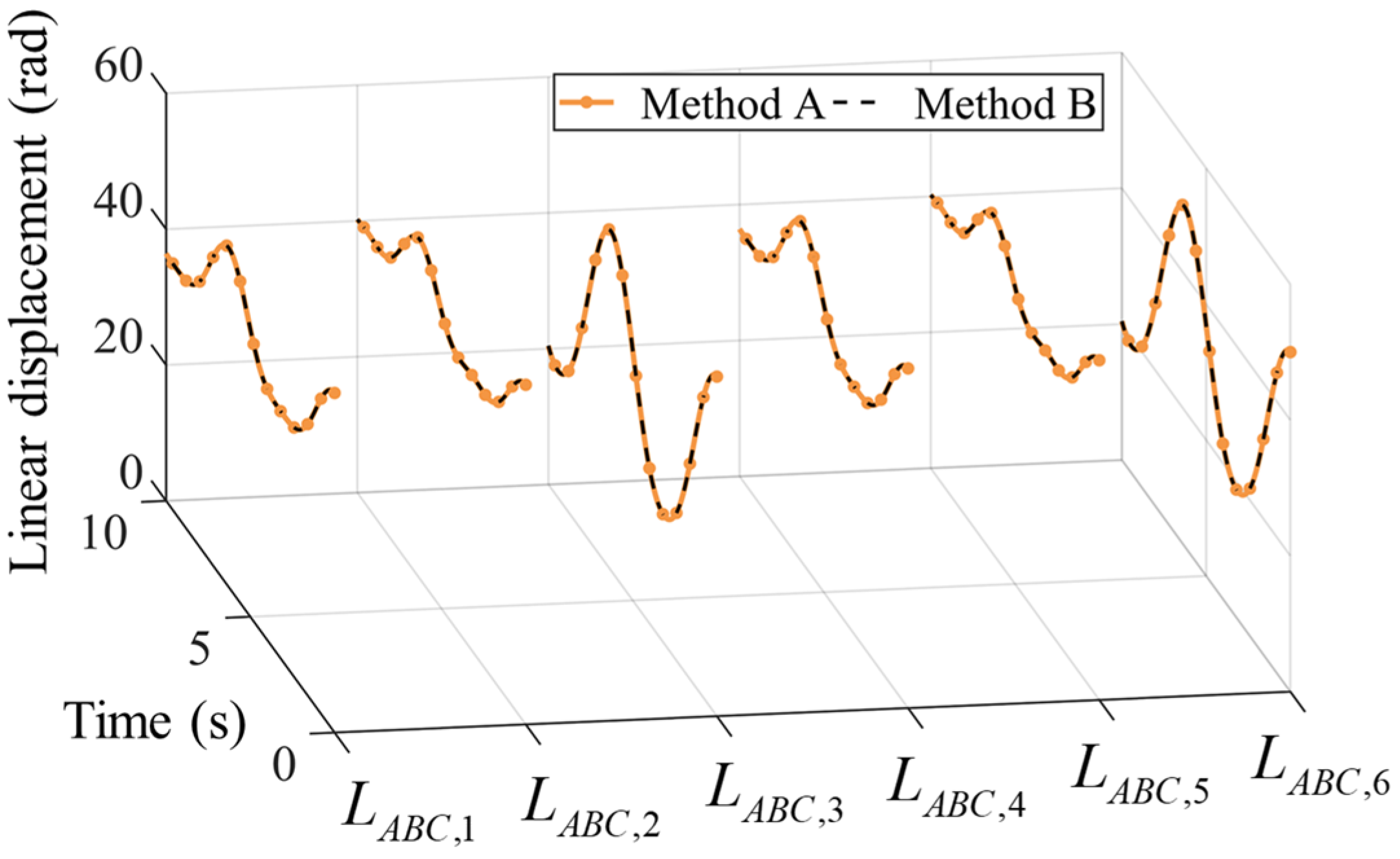
To further verify the correctness of the results simulated using the proposed modeling method here, another numerical analysis based on the method introduced by Gallardo-Alvarado is also performed [29]. Method A represents the method using the unified modeling method proposed in this paper, and Method B is the method introduced by Gallardo-Alvarado. From Figure 12 and Figure 13, the results of both methods are consistent, which validates both methods.

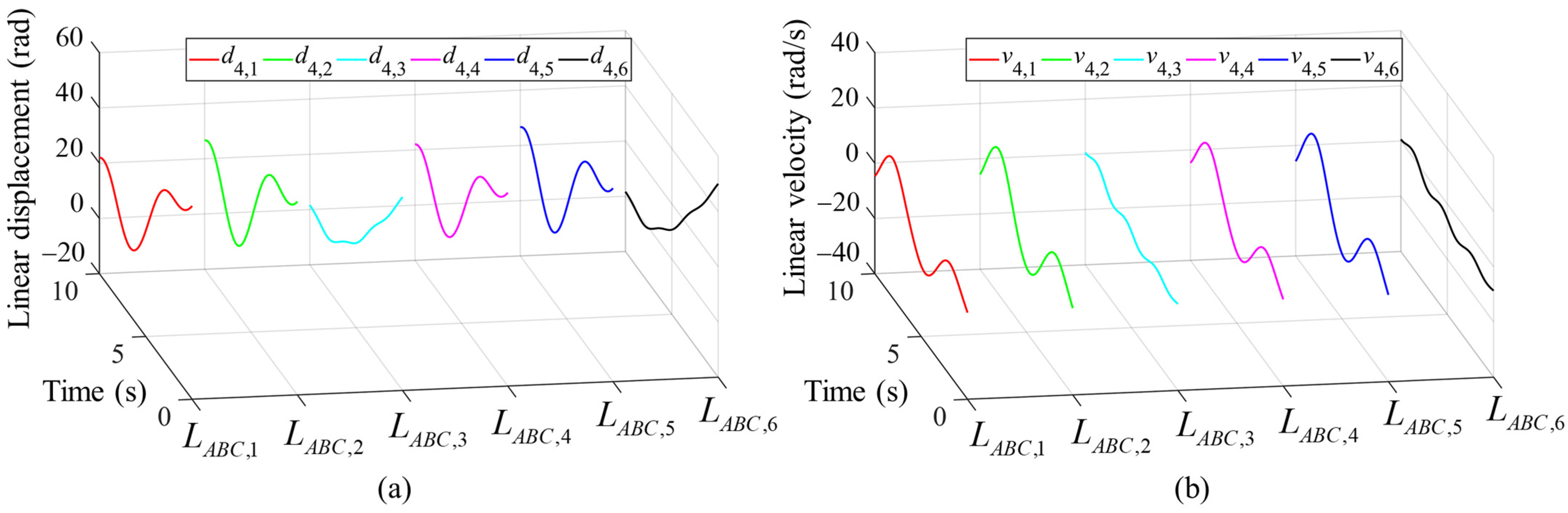
Besides demonstrating a simple circular trajectory, a more complex motion of the geometric center of the moving platform is given to show the performance of the method in analyzing the characteristics of a real mechanism. Some terms are added to simulate chaotic motion, and the velocity screw of the moving platform can be expressed as

$${}_0\mathsf{\$}_{iu}={\left[\begin{array}{cccccc}0& 0& 1& n\Delta t& -10\sin \left(n\Delta t\right)+\cos (n\Delta t)& -20\sin \left(n\Delta t\right)\end{array}\right]}^T$$

(34)

The same external loads acting on the geometric center of the moving platform are applied. The kinematics and statics analysis results are plotted in Figure 14, Figure 15 and Figure 16. Figure 14 gives the angular displacements (Figure 14a) and angular velocities (Figure 14b) of each revolute joint in six kinematic chains within the whole motion period. Because of the additional terms in the motion, the displacement and velocities are no longer periodic.

Figure 15 describes the linear displacements (Figure 15a) and linear velocities (Figure 15b) of the linear pairs within each kinematic chain.

Through the same static analysis approach, the driving forces ${\mathit{F}}_{B,i}$ to maintain the posture of the mechanism and keep the equilibrium within the complex motion period are analyzed. In Figure 16, the driving forces are in a reasonable arrangement and are adjusted during the motion. There are no sudden changes in either kinematic or static parameters, and the results show the working characteristics of the mechanism under complex motion requirements and external loads.

6. Conclusions

This paper proposes a unified screw kinematic and static analysis method and takes the Gough–Stewart platform as an illustrative example to investigate the kinematics and statics in screw coordinates. The velocity screw of a single rigid body is composed of angular velocity and linear velocity to express the general motion of a linkage, and the force screw of a single rigid body is composed of force and torque to express the general force of a linkage. The velocity screw equation indirectly provides the absolute position and posture of each joint at any time, while the force screw equation establishes the equation of external loads exerted on the linkage using the unit screw matrix obtained in kinematic analysis. Based on the fact that the resultant wrench of external loads and the self-weight of a rigid object in equilibrium should be zero, the static equilibrium equation of the Gough–Stewart platform is established and expressed in the form of screws. In this paper, the kinematic and static analyses are unified in screw coordinates. This theoretical method provides great convenience for the kinematics and statics of spatial mechanisms. Utilizing the velocity in screw form as a global variable and expressing all parameters in screw coordinates enables easier programming and debugging via directly calling the parameters. The advantages of using velocity in screw form can be seen, especially in dynamic analysis, because the second-order differential interpolation can be avoided. Furthermore, feedback control strategies could be developed according to the kinematic and static parameters.

References

1. Dasgupta, B.; Mruthyunjaya, T.S. The Stewart Platform Manipulator: A Review. Mech. Mach. Theory 2000, 35, 15–40. [Google Scholar] [CrossRef]
2. Fichter, E.F.; Kerr, D.R.; Rees-Jones, J. The Gough—Stewart Platform Parallel Manipulator: A Retrospective Appreciation. Proc. Inst. Mech. Eng. Part C J. Mech. Eng. Sci. 2009, 223, 243–281. [Google Scholar] [CrossRef]
3. Furqan, M.; Suhaib, M.; Ahmad, N. Studies on Stewart Platform Manipulator: A Review. J. Mech. Sci. Technol. 2017, 31, 4459–4470. [Google Scholar] [CrossRef]
4. Liu, X.; Wiersma, R.D. Optimization Based Trajectory Planning for Real-Time 6DoF Robotic Patient Motion Compensation Systems. PLoS ONE 2019, 14, e0210385. [Google Scholar] [CrossRef] [PubMed]
5. Galván-Pozos, D.E.; Ocampo-Torres, F.J. Dynamic Analysis of a Six-Degree of Freedom Wave Energy Converter Based on the Concept of the Stewart-Gough Platform. Renew. Energy 2020, 146, 1051–1061. [Google Scholar] [CrossRef]
6. Horoub, M.M.; Hassan, M.; Hawwa, M.A. Workspace Analysis of a Gough-Stewart Type Cable Marine Platform Subjected to Harmonic Water Waves. Mech. Mach. Theory 2018, 120, 314–325. [Google Scholar] [CrossRef]
7. Keshtkar, S.; Poznyak, A.S.; Hernandez, E.; Oropeza, A. Adaptive Sliding-Mode Controller Based on the “Super-Twist” State Observer for Control of the Stewart Platform. Autom. Remote Control 2017, 78, 1218–1233. [Google Scholar] [CrossRef]
8. Fry, S.T.; Turner, C.J. Design of a Stewart-Gough Platform for Engineering Material Characterization. In Proceedings of the ASME 2014 International Mechanical Engineering Congress and Exposition, Phoenix, AZ, USA, 11–17 November 2016; American Society of Mechanical Engineers: New York, NY, USA, 2016; Volume 11, p. V011T15A034. [Google Scholar]
9. Gan, D.; Dai, J.S.; Dias, J.; Seneviratne, L. Forward Kinematics Solution Distribution and Analytic Singularity-Free Workspace of Linear-Actuated Symmetrical Spherical Parallel Manipulators. J. Mech. Robot. 2015, 7, 041007. [Google Scholar] [CrossRef]
10. Dai, J.S.; Jones, J.R. A Linear Algebraic Procedure in Obtaining Reciprocal Screw Systems. J. Robotic Syst. 2003, 20, 401–412. [Google Scholar] [CrossRef]
11. Lu, Y.; Li, X.; Zhang, C.; Liu, Y. Analysis of Kinematics and Statics for a Novel 6-DoF Parallel Mechanism with Three Planar Mechanism Limbs. Robotica 2016, 34, 957–972. [Google Scholar] [CrossRef]
12. Shen, H.; Chablat, D.; Zeng, B.; Li, J.; Wu, G.; Yang, T.-L. A Translational Three-Degrees-of-Freedom Parallel Mechanism With Partial Motion Decoupling and Analytic Direct Kinematics. arXiv 2020, arXiv:2002.02964. [Google Scholar] [CrossRef]
13. Zhao, J.-S.; Wei, S.-T. Kinematics of Articulated Planar Linkages. Front. Mech. Eng. 2021, 7, 774814. [Google Scholar] [CrossRef]
14. Zhang, Z.; Xie, G.; Shao, Z.; Gosselin, C. Kinematic Calibration of Cable-Driven Parallel Robots Considering the Pulley Kinematics. Mech. Mach. Theory 2022, 169, 104648. [Google Scholar] [CrossRef]
15. Kanaan, D.; Wenger, P.; Chablat, D. Kinematic Analysis of a Serial–Parallel Machine Tool: The VERNE Machine. Mech. Mach. Theory 2009, 44, 487–498. [Google Scholar] [CrossRef]
16. Saafi, H.; Laribi, M.A.; Zeghloul, S. Forward Kinematic Model Improvement of a Spherical Parallel Manipulator Using an Extra Sensor. Mech. Mach. Theory 2015, 91, 102–119. [Google Scholar] [CrossRef]
17. Hu, B. New Approach for Analyzing the Stiffness of 3-RPS Parallel Manipulator. JME 2010, 46, 24. [Google Scholar] [CrossRef]
18. Hong, M.B.; Kinestatic, Y.J.C. Analysis of Nonsingular Lower Mobility Manipulators. IEEE Trans. Robot. 2009, 25, 938–942. [Google Scholar] [CrossRef]
19. Lu, Y.; Hu, B.; Yu, J. Analyses of the Stiffness and Elastic Deformation of a 2(3-SPR) Serial—Parallel Manipulator. Proc. Inst. Mech. Eng. Part K J. Multi-Body Dyn. 2009, 223, 189–198. [Google Scholar] [CrossRef]
20. Kong, X.; He, X.; Li, D. A Double-Faced 6R Single-Loop Overconstrained Spatial Mechanism. J. Mech. Robot. 2018, 10, 031013. [Google Scholar] [CrossRef]
21. Yang, T.-L.; Liu, A.; Shen, H.; Hang, L.; Jeffery Ge, Q. Composition Principle Based on Single-Open-Chain Unit for General Spatial Mechanisms and Its Application—In Conjunction With a Review of Development of Mechanism Composition Principles. J. Mech. Robot. 2018, 10, 051005. [Google Scholar] [CrossRef]
22. Kong, K.; Chen, G.; Hao, G. Kinetostatic Modeling and Optimization of a Novel Horizontal-Displacement Compliant Mechanism. J. Mech. Robot. 2019, 11, 064502. [Google Scholar] [CrossRef]
23. Zhao, J.-S.; Wei, S.-T.; Ji, J. Kinematics of a Screw Linkage. SN Appl. Sci. 2021, 3, 876. [Google Scholar] [CrossRef]
24. Zhao, J.-S.; Wei, S.; Ji, J. Kinematics of a Planar Slider-Crank Linkage in Screw Form. Proc. Inst. Mech. Eng. Part C J. Mech. Eng. Sci. 2022, 236, 1588–1597. [Google Scholar] [CrossRef]
25. Shai, O.; Pennock, G.R. A Study of the Duality Between Planar Kinematics and Statics. J. Mech. Des. 2006, 128, 587–598. [Google Scholar] [CrossRef]
26. Zhao, J.-S.; Wei, S.-T.; Sun, H.-L. Kinematics and Statics of a 3- UPU Robot in Screw Coordinates. J. Mech. Robot. 2023, 15, 061004. [Google Scholar] [CrossRef]
27. Zhao, J.; Feng, Z.; Chu, F.; Ma, N. (Eds.) Advanced Theory of Constraint and Motion Analysis for Robot Mechanisms; Academic Press: Waltham, MA, USA, 2014; ISBN 978-0-12-420162-0. [Google Scholar]
28. Dai, J. Historical Relation between Mechanisms and Screw Theory and the Development of Finite Displacement Screws. JME 2015, 51, 13. [Google Scholar] [CrossRef]
29. Gallardo-Alvarado, J. Kinematic Analysis of Parallel Manipulators by Algebraic Screw Theory; Springer International Publishing: Cham, Switzerland, 2016; ISBN 978-3-319-31124-1. [Google Scholar]
Figure 1. Geometry of a Stewart platform: (a) vertical view; (b) front view.
Applsci 13 10150 g001
Figure 2. Open kinematic chain.
Applsci 13 10150 g002
Figure 3. Closed kinematic chain.
Applsci 13 10150 g003
Figure 4. Kinematics analysis of the Gough–Stewart platform: (a) kinematic modeling of Gough–Stewart platform; (b) kinematic expressions of a single chain.
Applsci 13 10150 g004
Figure 5. Statics of kinematic chain.
Applsci 13 10150 g005
Figure 6. Procedure of kinematics and statics analysis of serial kinematics chain.
Applsci 13 10150 g006
Figure 7. Statics of Gough–Stewart platform: (a) statics of the Gough–Stewart platform; (b) statics of one fixed leg; (c) statics of the moving platform.
Applsci 13 10150 g007
Figure 8. The given circular trajectory of the moving platform and the external loads on the Gough–Stewart platform.
Applsci 13 10150 g008
Figure 9. The kinematics of each revolute pair through following the circular path: (a) angular displacement; (b) angular velocity.
Applsci 13 10150 g009
Figure 10. The kinematics of each prismatic pair through following the circular path: (a) linear displacement; (b) linear velocity.
Applsci 13 10150 g010
Figure 11. Driving forces of prismatic pairs F B , i of each chain through following the circular path.
Applsci 13 10150 g011
Figure 12. The linear displacements of each prismatic pair through following the circular path simulated using two methods.
Applsci 13 10150 g012
Figure 13. Driving forces of prismatic pairs F B , i of each chain through following the circular path simulated using two methods.
Applsci 13 10150 g013
Figure 14. The kinematics of each revolute pair through following the complex path: (a) angular displacement; (b) angular velocity.
Applsci 13 10150 g014
Figure 15. The kinematics of each prismatic pair through following the complex path: (a) linear displacement; (b) linear velocity.
Applsci 13 10150 g015
Figure 16. Driving forces of prismatic pairs F B , i of each chain through following the complex path.
Applsci 13 10150 g016