Article

PV Sizing for EV Workplace Charging Stations—An Empirical Study in France

by
Bruno Robisson
1,*,
Van-Lap Ngo
1,
Laurie Marchadier
1,
Mohammed-Farouk Bouaziz
2 and
Alexandre Mignonac
1
1
Commissariat à l’Energie Atomique et aux Energies Alternatives (CEA), CEA Cadarache, 13108 Saint-Paul-lèz-Durance, France
2
University Grenoble Alpes, CEA, Liten, INES, 50 Av. du Lac Léman, 73370 Le Bourget-du-Lac, France
*
Author to whom correspondence should be addressed.
Appl. Sci. 2023, 13(18), 10128; https://doi.org/10.3390/app131810128
Submission received: 7 July 2023 / Revised: 1 September 2023 / Accepted: 4 September 2023 / Published: 8 September 2023
(This article belongs to the Special Issue Photovoltaic Power System: Modeling and Performance Analysis)

Abstract

:
Photovoltaic (PV) powered Electric Vehicle Charging Stations (PVCS) have received extensive attention recently due to the complementary relationship of PV energy and electric vehicles. This paper proposes a methodology aimed at assisting a Charging Point Operator (CPO) in determining the size of the main components of such PVCS. The modular structure of the method gives flexibility for possible use on a new sizing problem by modifying key parameters such as the EV charging demand (i.e., arrival/departure times and energy needed to fill the battery), the EV charging strategy or the business model, independently from each other. It is of particular interest for a CPO that sizes many PVCS operated in the same environment (for example, a car park at a workplace). In that case, the CPO first has to apply the method on a representative charging station. Next, he can re-use parts of the obtained results to drastically speed up (from weeks to hours) the sizing of the other charging stations. The proposed method has been applied to the EVCS of an industrial research complex in southern France. The input dataset used to apply the method consists of more than 32,000 charging transactions spanning over 6 years with 350 EV users and 80 charging points. Three charging strategies with different levels of complexity are investigated, including Mean Power, Plug and Charge, and Solar Smart Charging. The considered business model is based on the maximization of the self-production rate. The numerical findings reveal that employing a straightforward charging strategy, such as Mean Power, leads to a substantial reduction of nearly half in the required size of the PV plant compared to the basic Plug and Charge mode. In addition, our analysis demonstrates that Solar Smart Charging has the potential to decrease the PV plant size by nearly three times.

1. Introduction

On 4 November 2022, the French Senate enacted legislation mandating exterior parking stations for light-duty vehicles exceeding 1500 square meters to allocate at least 50% of their surface area to solar panels [1]. The French government has also established a series of financial incentives to accelerate the transition towards a sustainable transportation sector, encompassing both the purchase of electric vehicles and the installation of charging infrastructure. These legal obligations and incentives collectively pave the way for the widespread adoption of energy systems that integrate both PV and EV. Reviews of all the possible interactions between these two technologies are provided in [2,3,4,5]. Amongst all these possible interactions, we consider that large PV-powered EV Charging Stations (PVCS) near workplaces are one of the most promising use-cases. First, from a technical point of view, in such a case, the EV charging demand (that lasts all the working day long) is “nearly” concurrent to the PV production. Second, if the number of EVs is large enough, this demand is also rather predictable. These two points a priori facilitate the optimization of the PV energy use. This use-case is also one of the simplest in terms of interactions between the stakeholders, rendering their cooperation possible, as proven experiments described in [6] and on a larger scale ten years later in [7]. Furthermore, when the PVCS are large enough (both in terms of PV capacity and the number of charging points), it takes advantage of the scale effect on costs. Finally, when the PV panels make car park canopies, the PVCS provides a better customer/worker experience (by shading the user’s car and by offering EV charging service) and promotes the energy transition.
In the context of large PVCS, several technical and financial stakeholders interact with each other [2]. An EV Charging Infrastructure (EVCI) with multiple charging points is managed by a Charging Point Operator (CPO). For the sake of simplicity, we consider that the EV driver interacts directly with the CPO, even if, in practice, another stakeholder called e-MSP (for e-Mobility Service Provider) sometimes acts as a third party between the CPO and the driver. Within the vicinity of the EVCI, ground-mounted PV plants and/or solar carports are installed and operated by a Photovoltaic Operator (PVO). In order to be as generic as possible, we assume that PVO and CPO are distinct legal entities. We consider that the PV plant and the charging stations are both connected to the distribution network, managed by the Distribution System Operator (DSO), but are associated with two different connection points (i.e., they have two different power meters). These power connections serve a dual function; they provide power to the EV stations during periods of insufficient PV generation and enable the surplus PV energy to be injected into the grid when there is an excess of production.
Sizing PVCS at the earliest design step is crucial, especially for the CPO, because such sizing will be the basis for the next design phases. However, this step is a particularly difficult task. First, by essence, the technical details of the final PVCS, such that the IT and power architecture and the EV charging control algorithms (if any), are unknown. Thus, during the sizing phase, the designer has to choose models that not only have to be “rough” (i.e., that do not include technical details) but also have to correspond to feasible and practical technical solutions. Second, data about the EV demand (i.e., arrival/departure times and energy needed to fill the EV batteries) that spans a large time horizon (at least half or one year) is key data to size the PVCS. In general, such data is not available or is of poor quality at this stage. Third, many business interactions between the different stakeholders can be imagined, rendering the formalization of a generic sizing method rather difficult.
The objective of this paper is to provide a method that encompasses these difficulties. First, the “rough” models of the PVCS used in this paper are based on more than ten years of expertise in analyzing the interactions between PV and EVs at CEA. In particular, this paper takes into account three different EV charging strategies. The most complex one sketches a strategy that has been validated in practice with real users in two different places [6,7]. Second, the method proposed in this paper is based on four relationships that can be studied independently from each other. One of them determines which part of the EV annual consumption comes from the PV, given the number of EVs, a charging strategy and the size of the PV plant. This relationship is determined in this paper thanks to a massive empirical dataset collected over more than 6 years, from 1 June 2016 to 31 August 2022, with 350 EV users and 80 charging points at the workplace. Computing this relationship requires time and resources. However, it can be re-used for PVCS that are in the same context (i.e., a large car park at a workplace). The use of such pre-computations drastically speeds up the time needed to apply the method (from several days to several hours). This property may be, for example, particularly interesting for a CPO that has to size several charging stations with approximately the same EV charging demand. Third, one of the four relationships is specific to a given financial exchange between the stakeholders. This relationship may be adapted easily to different business cases without changing the other relationships. To the best of our knowledge, the method proposed in this paper is the only one that has such properties.
The remainder of the paper is organized as follows: Section 2 describes the state of the art research on this topic and highlights our main contributions. Section 3 summarizes the proposed methodology, context, input data and variables. Section 4 details the computation of the different relationships between input and variables. These relationships are related to (1) the business models (i.e., stakeholders and their interactions); (2) the EV consumptions; (3) the PV production and forecast; and (4) the charging strategy. Section 5 presents numerical examples of the methodology, while Section 6 provides an overview of the results with the perspectives of the study. Finally, an Appendix A section is made to model the relationship between the Production-to-Consumption ratio and the Self Production Rate.

2. State of the Art

2.1. Research Positioning

There are four stages in the procedure of project development of an energy system [8].
  • The first one is the “idea development.” It consists of “brainstorming and idea generation activities to give the project a more rounded shape”;
  • The second one is the “concept development” which describes the scope of the project (case descriptions, investment context, system and stakeholder overviews, etc.). It also specifies the resources required and estimates key financial (such as revenue stream, CAPEX, OPEX, etc.) and technical figures. Amongst them, the size of the main components of the system is determined. For example, the sizing of PVCS consists in determining one or all of the following quantities: the maximum power that the PV plant may deliver (also called “peak power”), the number of charging points (and possibly the maximum power that each of these charging points may deliver), the number of EVs that may be charged on the PVCS, or the capacity and the maximum power of the storage system. For such sizing studies, EV demand (number of daily EVs and their arrival and departure time), users’ behavior, and vehicles’ characteristics are the most imperative type of input data. Other types of input data are also required, such as incentives, taxes, grid codes, PV potential, etc. The concept development phase also determines the project risks, its social and environmental impacts and its profitability;
  • The third stage is called “business development” and outlines all the actions needed to make “real” the system sketched during the previous phase. During this phase, the system is first designed in detail and an operation plan to build it is provided;
  • The last stage is dedicated to the project execution. This phase entails the construction and installation of the final system, plus any other civil work needed for the project operations.
The concept development phase usually consists of a prefeasibility study (PFS) and a feasibility study (FS). As explained in [8], “the PFS scans a series of options and determines the best one in the set. The FS analyzes in depth the best solution from the prefeasibility phase. The PFS reduces the number of options that are chosen to proceed with a more detailed feasibility study and eventually with business development, ultimately saving time and money”.
The objective of this paper is to provide a method to size PVCS during the early steps (i.e., during the PFS) of the concept development phase. As explained in [9], such sizing is particularly crucial, especially for the CPO, because it is considered a strong basis for the business development phase. Such sizing is a particularly difficult task because many of the details of the final system are not known. For example, much data necessary for sizing the PVCS is not available or is of poor quality at this stage. To circumvent this difficulty, EV demand could, for example, be synthesized from statistical distributions derived from experimental data [10]. However, due to daily and seasonal variations, this data also have to span a large time horizon (at least half or one year). Moreover, the details of the power infrastructure, of the IT architecture and of the control system that will be implemented on the final system are also generally not known. In the following, the term “control system” covers the algorithms (classified into scheduling, clustering and forecast in [11]) and all the interactions with the IT and the power systems that aim at optimizing the PVCS functioning for a given objective (expressed in terms of financial, efficiency and environmental [4]). Thus, the person who conducts the concept development phase has to use models of the control system that describe the behavior of the final one in a way as relevant as possible, but such models also have to be simple enough to explore many design possibilities [12].
The following section describes the state of the art on the problem of sizing during the concept development phase of energy systems that integrate at least both EVs and PV (in the context of micro-grid or not). In particular, we do not take into account works focusing solely on the design of the control algorithm. The reader could find such references in Table 1 of [9] (column ‘optimal control’).

2.2. Sizing PVCS at the Concept Development Step

The study in [9] details the sizing of the main components of a system constituted of a household, a battery, a PV plant and bidirectional EV chargers. Three EVs with identical parking time schedules during weekdays (8 a.m.–6 p.m.) are considered. The authors integrate the sizing problem into the optimal power management problem by considering, in addition to the EV and battery power profiles, the components ratings as decision variables. These variables are the BES capacity (kWh) and their charger power ratings (kW), the PV system power rating (kW), the inverter power rating (kW) and the EV charger power rating (kW). Power management minimizes the costs (including those due to battery degradation) by taking into account network and component constraints. Such constraints allow for elaborate business models based on self-consumption, energy arbitrage and FCR market participation. The optimization algorithm is formulated and implemented in GAMS (Generic Algebraic Modeling System) [13].
The authors in [14] propose an optimal sizing-control methodology for residential microgrids where EVs are viewed as controllable loads. The microgrid contains PV, Wind Turbines (WT), a bidirectional inverter and a local Battery Energy storage System (BES). The optimization algorithm is based on Mixed Integer Linear Programming (MILP) and solved using CPLEX [15]. It is designed to minimize the annual cost of electricity. The size of the components are the decision variables of this algorithm, in addition to the dispatched power profile. In this paper, the number of EVs is fixed and, so, is not considered as part of the sizing decision variables. EV mobility data include three EVs with a deterministic nature.
The authors in [16] identified the optimal sizes of PV, WT and BES in a smart home microgrid configuration and vehicle-to-home context. The energy management system aims at minimizing the annual cost of electricity, and it follows rule-based logic, whereas the sizing problem utilizes the particle swarm optimization technique [17]. The meteorological and EV mobility data (for one single vehicle) are randomly generated (based on probabilistic distribution functions obtained from various datasets).
The authors in [18] study a microgrid made of an EV charging station, a BES and a PV plant. This microgrid is located at a workplace. The operation of the charging stations is controlled using customized expert rules that aim to minimize the energy fed/drawn from the grid. The authors propose a methodology for determining the optimal PV panel tilt and the BES size for two scenarios and for eight different charging profiles. The optimal values are found by testing a set of values in a given range and selecting the value that gives the best results. In this paper, for example, the author tests the capacity of the BES from 5 kWh to 75 kWh by steps of 5 kWh. Such a technique that tests a given set of parameters will further be called “parametric analysis”.
In [12], the authors consider a system constituted of a PV plant and EVs (that embed bidirectional chargers). In one of their numerical examples, they consider a 2.64 MWp plant and 184 EVs. The algorithm that controls the charge/discharge of the EV is designed to minimize the difference between the day-ahead production commitment of the PV plant and its real production. The optimization problem is formulated as a linear optimization problem. The authors consider a deterministic charging demand, i.e., all the vehicles are supposed to be available from 9 a.m. to 6 p.m. Lastly, they compared the results of their control algorithm for different ratios between the number of EVs and the peak power of the PV plant.
An economic study of EV parking lots at workplaces equipped with PV in the states of Ohio and California in the US [19] was conducted to demonstrate the economic attractiveness of such an installation with different PV installed capacities and financial hypothesis. Vehicle mobility data (arrival time, parking time) are statistically simulated using probability distributions derived from the Ohio State University’s parking garage empirical data. Various incentives and tax deductions from multiple levels of authority are taken into consideration for the financial model. MatlabTM is utilized for EV charging demand simulation and grid emission, while PV production and cash flow computation are performed in the System Advisor Model (SAM) [20,21]. A constant 6.6 kW charging power is simulated in this case. To follow up with this, the authors also conducted a similar study with a more sophisticated charging algorithm using dynamic programming and optimization technics [22]. This algorithm maximizes the use of PV energy and reduces the impact on the grid while satisfying the energy demand of EVs. Parametric analyses are conducted with multiple varying factors (PV size, PV installation costs, incentives, electricity rates, parking rates) to study their financial impacts (mainly in terms of payback time).
The work in [23] presents a methodology for sizing different energetic components of a PVCS in the microgrid context, including the size of the PV system, the stationary battery systems and the transformer. Theses sizes and other operational constraints are part of the objective function of an optimization algorithm that aims to minimize the entire system’s economic costs. The EVs’ initial SOCs are assumed to follow Gaussian distribution within the range of 0.2 and 0.5. The EVs’ battery capacities, number of daily EVs and arrival time are also synthesized using Gaussian distributions. The paper concluded that with this methodology, the cost of the optimally sized configuration without PV would be higher than that of an optimal configuration with PV installation. In one of their numerical examples, they consider a charging station made of four chargers of 40 kW each, a 300 kWp plant, a 600 kWh battery and a 200 kW transformer.
The authors in [24] introduced a rather simple multi-phased methodology to size a microgrid made of a PV plant, a BES and a charging station. This method is formalized with an Excel-based tool customized for various stakeholders and authorities. The customization of EV charging profiles and of physical as well as financial parameters allows users from different backgrounds to efficiently analyze the performance of the charging infrastructure from multiple aspects. The energy management strategy in this work is rather straightforward and representative of the real deployment strategy: energy from the grid would be required if PV production (and sequentially a stationary battery system production) is insufficient. However, if PV production surpasses the EV demand, then the surplus would be stored in the stationary battery or injected into the grid if there is still excess energy. The aim of this control is to avoid overloading the power grid and guarantee a high percentage of PV energy.
In [25], the authors study the integration of EV and PV in an office building located in southern Italy. In this study, one EV is charged during working hours. Four different charging needs are considered (from 0 km per day to 120 km per day). They also compare two charging modes: the first one is an AC charge without control, and the second one is a DC charge with control such that the EV consumes the surplus of the PV production. The authors compute the self-consumption and self-production rates obtained for four different values of PV peak powers (from 4.5 kWp to 9 kWp) for the two charging modes and for different sizes of charging points.
In [26], the authors study the integration of EV and PV in a household. Several scenarios are simulated over a long-term period (ten years) in order to take into account the aging of the battery and the PV panels. The parameters that distinguish the scenario are the yearly driving distance of EV users (from 10,000 km per year to 25,000 km per year), the charging strategy (uncontrolled or basic control that increases the self-production) and the location and size of the PV plant (varies from 2 kWp to 10 kWp). The last parameter is the type of EV user: he is either a commuter who is not parked at home during working days or a “private user” who, on the contrary, returns home several times a day. The EV charging profiles associated with these types of users are synthetized from statistics described in [27].

2.3. Synthesis

The authors in [2] propose to distinguish systems that integrate PV and EV according to three criteria:
  • Their spatial configuration. The authors distinguish systems that span over households, buildings, charging stations or territories. We also propose to add the size of the PV plant and the number of EV users as criteria;
  • Their technological environment. It consists of the technological components that are included in or are added on. Such components could be BES, WT, Heat Ventilation Air Conditioning (HVAC), network technologies (such as DC micro-grids), etc.;
  • Their smart control strategy. The authors in [2] also distinguish the strategies by their objectives that can be expressed in monetary terms (such as maximizing the revenues or minimizing electricity costs, etc.), in energy efficiency terms (such as improving self-consumption or reducing the impact on the grid) or in ecological footprint terms (such as reducing the CO2 emissions). The authors also distinguish the strategies by their “coordination method”, that is, their mathematical formulation. These methods could be based on “optimization methods” (such as MILP, etc.), “heuristics methods” (such as those based on expert rules) or “hybrid methods” (i.e., a combination of the two previous methods).
As explained in Section 2.1, prefeasibility studies aim at exploring several potential solutions, whereas feasibility studies focus on the most promising ones. In practice, the two phases are distinguished by their levels of complexity, specifically in terms of required data and level of expertise. The level of expertise is mainly about the complexity of the charging schedule algorithms and the software that is used for their implementations. Heuristics methods are mostly used during prefeasibility studies, whereas optimization methods are rather used in feasibility studies.
Table 1 summarizes these reviewed papers in Section 2.2 using the aforementioned criteria along with additional ones: targeted project development stage, EV fleet and PV size, EV mobility data, sizing methods, and the variables/parameters to be sized.
Table 1. Summary of literature review: Abbreviations: FS = Feasibility Study, PFS = Prefeasibility Study, CS = Charging Station, MILP = Mixed Integer Linear Programming, LP = Linear Programming, DP = Dynamic Programming, PSO = Particle Swarm Optimization.
[9][14][16][18][12][22][23][24][25][26]This work
Development StageFSFSPFSPFSFSFSPFSPFSPFSPFSPFS
Spatial ConfigurationHouseholdResidential MicrogridHouseholdCSCSCSCSCSOfficeHouseholdCS
Fleet and PV Size3 EVs
From 0 to 50 KWp of PV
Hundreds of EVs
Hundreds KWp of PV
1 EV
Several kWp of PV
1 EV
Several kWp of PV
Dozens to hundreds of EVs
Dozens to thousands KWp of PV
Dozens to hundreds of EVs
Dozens to thousands KWp of PV
Several EVs Hundreds kWp of PVSeveral EVs Several KWp of PVOne EV
4.5 kWp to 9 kWp of PV
One EV
Several KWp of PV
Dozens to hundreds of EVs
Dozens to thousands KWp of PV
EV Mobility DataDeterministicDeterministicProbabilisticDeterministicDeterministicProbabilisticProbabilisticUser definedDeterministicProbabilisticEmpirical
ComponentsPV, BES, EV ChargerPV, WT, BESPV, WT, BESPV, BESPV, EVPV, EVPV, BES, TransformerPV, BES, EVBuilding, PV, HVAC, EVPV, EVPV, EV
Control AlgorithmNonlinear OptimizationMILPRule-basedRule-basedLPDPMILPRule-basedRule-basedRule-basedRule-based
Sizing AlgorithmNonlinear OptimizationMILPOptimization (PSO)Parametric AnalysisParametric AnalysisParametric AnalysisMILPParametric AnalysisParametric AnalysisParametric AnalysisParametric Analysis
Sized VariablesPV, BES, EV Charger RatingsPV, WT, BES sizesPV, WT, BES RatingsBES RatingsPV Ratings, #EVPV RatingsPV, BES, Transformer RatingsPV, BES, EV Charger RatingsPV, EV Charger RatingsPV RatingsPV, #EV
ToolGAMSCPLEX---Matlab and SAM-Customized ToolTRNSYSPVSOLMatlab

2.4. Our Contribution

We consider that the EV charging demand data are one of the most important input data in prefeasibility/feasability studies. More precisely, we think that, in order to obtain precise results, this EV charging demand has to be as “representative” as possible of the use-case under study. In particular, this data has to encounter the variability of the EV users’ behavior over a long period but also has to take into account the characteristics of the EVs and of the charging points. We also think that it could be possible to define “standard” EV charging demands corresponding to:
  • Workplace parking lots (where the EVs remain plugged in during work hours);
  • Shopping centers (where the users arrive all day long and stay only a couple of hours);
  • Residential (where the users arrive at the end of the day and leave in the morning);
  • Delivery fleet (where the EV arrives at a fixed time in the day and also leaves at another fixed time).
The workplace parking lots use-case illustrates this article; we have collected empirical data over a horizon of more than six years at an industrial and research complex in southern France. As detailed in Section 4.2, the dataset includes more than 32,000 transactions, 350 EV users, more than 40 EV models and 80 charging points. According to the literature review and to the best of our knowledge, this paper is the first that describes a sizing procedure based on a large and real EV charging dataset.
Furthermore, the computational logic of the proposed methodology can be split into four main relationships between input data and internal variables (defined in Section 3.3). Obtaining relationship 4, which relates the self-production ratio and the Production-to-Consumption ratio, is a rather complex task; the designer has to (1) collect and process input data (that are mainly the EV demand and the PV production and forecast), (2) perform simulations and (3) aggregate all the simulations results. Relationship 1 relates the price of the energy and the self-production rate. This relationship may be quite easily adapted to all the business models that aim at increasing this self-production rate. At last, relationships 2 and 3 are quite easy to compute. Thus:
  • When the PVCS designer assumes that the EV charging demand is a standard one, the pre-computations of relationship 4 can be re-used. The designer may also modify relationship 1 if the considered business model is not the same as the one described in this article. In the two cases, minimum effort, in terms of time and resources (i.e., a few hours for a non-specialist), is required;
  • When the designer encounters a specific use-case (i.e., non-standard), pre-processed data proposed in this paper is not usable. The four relationships of the methodology have to be computed. This level of involvement allows us to obtain an estimation of the project’s performance with the highest precision, but the effort is also the highest. We estimate that 3 or 4 weeks with decent programming competences are required.
In other words, the modular structure of our method enables us to modify the business models independently of the other parameters. It also enables to pre-compute intermediate results. Once these pre-computations are performed, the sizing procedure may be quick and simple. To our knowledge, this is the only method that has such properties. It is of particular interest, for example, for a CPO that will have to size many charging stations with approximately the same charging demand. In that case, the CPO will first have to compute all the relationships from the charging demand of a representative charging station. Next, he will re-use the relationships (in particular, the 4th) to drastically speed up the sizing of the other charging stations.

3. Context and Methodology

3.1. Use-Case: CEA Cadarache EV Charging Infrastructure (EVCI) and PV Plant

The data collection took place in the Cadarache research center of the French Alternative Energies and Atomic Energy Commission (otherwise known as CEA, the French acronym for “Commissariat à l’Énergie Atomique et aux Énergies Alternatives”) located near Aix-en-Provence. This research center disposes its own water, heating, lighting and electricity distribution network in which it operates as the DSO. A private bus service is offered to its employees for commuting and for trips between laboratories and canteens. A taxi service is also offered for intra-site trips. Thus, the Cadarache center can be seen as a town with a population of approximately 5000, privately owned and managed by CEA.
The CEA also set-up an EVCI during the summer of 2016. It involves 40 Diva-type terminals, produced and installed by G²Mobility, which was bought out by TotalEnergies in 2018. Each Diva terminal has two 22-kW AC charging points. Each of these charging points has a type 2 socket for mode 3 connection and a type E socket for mode 1 and 2 connections. These charging stations have been installed alone or in groups of up to four Diva terminals to create 30 charging stations spread throughout the center. Each charging station has an embedded IoT gateway that enables communication through 3G networks by using Open Charge Point Protocol (OCPP) commands. As soon as the EV is plugged in, it is charged at its nominal power. In other words, the EVCI lets the EV charge as rapidly as possible from the moment the vehicles are plugged in. This charging strategy, further named “Plug and Charge” strategy in this work, is generally the default strategy of most commercial charging points.
CEA also conducts research at Cadarache with INES on solar thermal energy and photovoltaics. In particular, CEA tests and evaluates innovative PV systems (such as Tandem Pérovskite-Silicium PV, bifacial PV, single- and dual-axis solar trackers) ranging in size from modules to a few tens of kW systems. The energy produced from all these pieces of equipment (which aggregates up to 50 kWp) is injected into the CEA private power network. Furthermore, the CEA plans to install other PV plants, either ground-mounted or on buildings, and to install PV solar shade. In this latter case, these PV plants will be sized for a self-consumption scheme, described in the following section.

3.2. Collective Self-Consumption Scheme

As explained in the introduction and visualized in Figure 1, we consider the general case where the EVCI and the PV installation are managed by two separate entities, namely the Charging Point Operator and PV Operator (CPO and PVO). The CPO has to manage the charging of a certain number of EVs while utilizing the production from the PV plant, characterized by a certain peak power, noted P P V p e a k . We also consider that they agree on an exchange of PV energy. Without loss of generality, this agreement could be a partnership with a ‘third party’ called Legal Person (LP), or Personne Morale Organisatrice (PMO) in French, according to the scheme called “collective self-consumption” in France. This LP entity plays the role of a facilitator for the financial as well as power flows between the CPO and the PVO. The CPO also contracts with an energy supplier (ESEV) that provides supplementary energy to the charging stations when PV production is insufficient to the EV charging consumption. In the meantime, the PVO also establishes a contract with another energy supplier (ESPV), which extracts the surplus PV energy produced when there is more PV production than EV consumption.
In this paper, the power x is denoted P x . The energy of P x over a period Δ , E x Δ is the integral of this power over Δ : ( E x Δ =   Δ P x d t ). The energy of the power P x calculated over a day, a month and a year are noted E x d , E x m and E x a , respectively. The energy of the power P x computed on an arbitrary period is noted without a subscript, i.e., E x . The price per kWh that actor A pays when he buys a given amount of energy from actor B is noted P r B A . It is important to note that this price may also include other services, apart from the energy production fee itself, such as transport, taxes and contributions.
With these notations (summarized in Table 2), the principle of this scheme, represented in Figure 2, is the following:
  • The PV power ( P P V ) and the corresponding energy ( E P V ), produced by the PV plant during the period, are visualized in the top left part of the figure;
  • The charging power ( P E V ) and energy ( E E V ) consumed by the EVs are represented on the bottom left diagram;
  • The CPO partially charges the EVs with the power P S P (SP for Self-Production) such that P S P = m i n P P V ,   P E V . The CPO buys the associated energy, represented in green and noted ESP to the LP at a price noted P r L P C P O ;
  • The PVO, for his part, sells ESP to the LP at a price noted P r P V O L P ;
  • The CPO also charges the EVs with the power P E S E V that complements P S P when there is not enough solar power (i.e., such as P E S E V = max ( P E V P P V ,   0 ) ). The CPO buys the associated energy, represented in dark blue and noted EESEV, to the power supplier ESEV at a price noted P r E S E V C P O ;
  • The PVO injects in the network the power P E S P V , if any, produced by the PV plant but not consumed by the EVS (i.e., such as P E S P V = max ( P P V P E V ,   0 ) ). The PVO sells the associated energy, represented in pink and noted EESPV, to the power supplier ESPV at a price P r P V O E S P V .
In such a configuration, the local DSO is responsible for the virtual dispatch (“virtual” because the dispatch is performed in front of the meter); the DSO measures E E V and E P V from the power meters of the EV charging point and the PV plants, respectively. The meters are read at a frequency that depends on the market time step whose value depends on countries. The DSO computes E E S P V ,   E E S E V ,   E S P based on the following logics and transfers these values to the LP, ESPV and ESEV, respectively.
  • E E S P V = max ( E P V E E V ,   0 )
  • E E S E V = max ( E E V E P V ,   0 )
  • E S P = min E P V ,   E E V

3.3. Main Internal Variables

The ratio between the total PV production to the total EV, computed for an arbitrary period, is termed Production-to-Consumption ratio (or PTC).
P T C = E P V E E V
We also consider the Self-Production Rate (SPR) and Self-Consumption Rate (SCR), which represent the proportion of total EV charging demand being supplied by the PV production and the proportion of total PV production used for EV charging, respectively. These variables are, for an arbitrary period, defined as follows:
S P R = E S P E E V
S C R = E S P E P V
Let us consider a period di such that the different prices are constant. The duration of such a period depends on the pricing scheme; if the prices are flat, the period is generally one year. On the contrary, if the prices are time-varying, the period is the market time step. The annual energy cost and the Mean Power Price, P r C P O   (€/MWh), which is the effective price of electricity that the CPO has to pay for both electricity from the PV and the electricity from the grid, are then calculated using Equations (4) and (5).
C o s t C P O a = d i Y e a r   E S P d i × P r L P C P O d i + E E S E V d i × P r E S E V C P O d i
P r C P O = C o s t C P O a E E V a

3.4. Methodology Description

3.4.1. Inputs/Output Data

This section describes the input data required, depending on the elements that are to be sized:
  • Given a target P r C P O (€/kWh) and a number of EV users, what should the PV peak power be (kWp)?
  • Given a PV peak power (kWp) and a number of EV users, what should the P r C P O be (€/kWh)?
  • Given a PV peak power (kWp) and a target P r C P O , what should be the maximum number of EV users?
The row name of Table 3 represents the targeted outputs, while the columns are the input data. For example, in order to calculate the peak power of a PV plant (first line of the table), 8 out of 9 inputs (marked with an X symbol) must be collected. The CPO has to provide the price of the power from the network ( P r E S E V C P O ) and from the PV plant ( P r E S P V C P O ); he also needs its target of Mean Power price ( P r C P O ), obtain data about potential PV production (location of the plant, orientation, tilt angle and possibly PV production and forecast profiles), the expected number of EVs and their main characteristics (size and efficiency of the embedded charger, capacity of the battery, etc.). He also needs a charging session history that contains, for each session, the start date and the end date of the session. This history also has to contain the energy withdrawn by the car during each session. The history also has to record the name of the charging point and the user’s badge number. Lastly, the CPO has to obtain the relationship between a badge and the EV model.

3.4.2. Principles

In this section, we briefly describe the main principles of the methodology, expressed in the form of four different relationships among different inputs, outputs and variables, as illustrated in Figure 3. First, we need to specify the energy exchange scheme between the CPO and the PVO. This scheme is then used to derive a relationship between the self-production rate (SPR) and the Mean Power price ( P r C P O ), with different prices as inputs. This first relationship is described in Section 4.1.
The charging session history is then used to express the annual EV energy consumption as a function of the number of EVs. This second relationship is then given in Section 4.2.
Next, we need to estimate the yearly PV production as a function of the PV peak power P P V p e a k . This production depends on the solar potential that varies with the location of the PV plant, its orientation and its tilt angle. Section 4.3 will specify more details about this relationship.
Lastly, we need the PV production forecast profile which is then combined with the charging session history to reconstruct the corresponding charging power profiles according to a given charging strategy. Based on these profiles and PV production profiles, we are able to compute the SPR. In addition, it is also possible to compute the Production-to-Consumption ratio, noted P T C . The relationship between the S P R and P T C is an abacus (that can then be approximated using empirical formulas as described in Appendix A), which is presented in Section 4.4.
The diagram in Figure 3 describes the computational logic flow for this methodology. The black plain line boxes are inputs and the dotted ones are inputs or outputs. The red boxes represent internal variables. Lastly, the bidirectional arrows represent the reciprocal relationship between two quantities (if one is known, the other can be determined and vice versa).

4. Relationships Necessary for the Application of the Method

4.1. Business Model

4.1.1. Hypothesis

We consider that P r E S P V = P r P V O L P in this paper, this means that all revenues of the PVO come with the same price, thus making its revenue independent of neither SPR nor SCR.

4.1.2. Relationship 1: Self-Production Rate versus Mean Power Price

The cost C o s t C P O given in Equation (4) can be rewritten by replacing E E S V E with E E S E V = E E V E S P = E E V S P R × E E V = E E V × ( 1 S P R ) , we obtain:
C o s t C P O = S P R × E E V × P r L P C P O + 1 S P R × E E V × P r E S E V C P O
The Mean Power price, previously given in Equation (5), is then obtained by dividing Equation (6) by E E V , thus establishing a linear relationship between P r C P O and SPR:
P r C P O = P r E S E V C P O S P R × P r E S E V C P O P r C P O L P
When P r E S E V > P r C P O L T , the Mean Power price for the CPO linearly decreases with the increasing value of SPR. In other words, if electricity from the PV plant is more affordable then from the grid, self-production has to be prioritized. When SPR = 0, P r C P O = E E V × P r E S V E . This means that when there is no PV available for EV charging, the Mean Power price is equivalent to the price of the power from the grid. When SPR = 1, P r C P O = P r C P O L P . This means that when there is no power coming from the network, the Mean Power price is the price of the power coming from the PV plant.

4.2. EV Consumption

4.2.1. Charging Periods

Data from 32,014 charging sessions were collected for more than 6 years, spanning from 1 June 2016 to 31 August 2022. Each charging session record contains the start and end time stamps of the session (noted ST and ET, respectively), the identification number (ID) of the charging point, the badge number of the user and the energy that has been supplied to the EV. The transaction duration, ET-ST, is denoted TD.
Figure 4 illustrates the distributions of the start and end times of the dataset. It is observed that the start time of the charging sessions is statistically concentrated around 8 a.m. (start of work hours), lunch time and early afternoon (after 4 p.m., when the business trips are terminated). There are also three main periods during which the majority of the charging sessions terminate. The first one is at 9 a.m. when the service cars that have been connected the day before are disconnected to be used for business trips, the second one is after lunchtime and the last period is at the end of the working day (around 5 p.m.) when employees leave the center. The average duration and energy consumption of each charging session were 11.3 h and 17.22 kWh, respectively, and a total of 551 MWh of electricity was consumed.

4.2.2. EV Users and EV Fleet Compositions

From the EVCI charging session history, we compute the number of “active” and “delivered” badges. A badge is said to be “active” from the start of its first charging session until the end of its last recorded session. The status “inactive” will be given otherwise. A badge is said to be “delivered” from its first connection to the EVSE. Figure 5 describes the number of active and delivered badges per day, where we can observe that 348 RFID badges were delivered for EV (including PHEV) owners and up to 200 active badges at the end of the considered period. Between 2021 and 2022, the number of delivered badges increased steadily by around 100 per year. At the end of the collection horizon, all the badges are inactive due to the definition of an active badge (i.e., they are all inactive after their last connection). It is also noted that there is a considerable amount of delivered inactive badges. This can be attributed to the loss of badges or to the fact that the users left them permanently or they stopped charging their EVs within the facility.

4.2.3. EV Characteristics

Technical information regarding the vehicle corresponding to the badge was also recorded: vehicle model and usage category (personal, internal taxi and service car). Amongst all the delivered badges, two hundred and thirty two vehicles are attributed to employees’ personal vehicles, eighty-four vehicles are for facility services and three Renault Zoé for internal taxi services. An additional 29 vehicles serving external companies are also among the considered EVs. In terms of car models, there is a very clear predominance of Renault Zoé, which represents 38% of the fleet. There are also, among others, 10% of Peugeot e208, 7% of Renault Twingo, 8% of Tesla (Model 3 and Model S) and 5% of Nissan Leaf vehicles.
Primary characteristics of vehicles were also collected from publicly available sources, namely, the nominal power of the on-board chargers (kW) and their battery capacity (kWh). Figure 6 displays the histogram of these nominal powers and battery capacities of the considered fleet. We observe that approximately 45%, 30% and 25% of EVs have nominal charging power at 22 kW, 11 kW and less than 11 kW, respectively. We also observe that more than half of the EVs have a battery capacity between 45 and 55 kWh.

4.2.4. Energy Consumption

From the EV charging session history, we have computed the aggregated daily, weekly, monthly, quarterly and annual energy delivered to the EVs. Figure 7 demonstrates that the total monthly energy consumption data can be classified into four groups over the entirety of the data collection. The first period, called pre-COVID-19, started in June 2016 and terminated at the beginning of the COVID-19 crisis. The second period corresponds to the first COVID-19 lockdown in France (March 2020–April 2020), during which very little charging service was used, leading to minimal electricity consumption. The third period (May 2020 to February 2022) has seen the introduction of the hybrid-working mode (i.e., normal onsite and work from home) and, thus, resulted in charging patterns similar to that of the first period but with slightly lower consumption. The last period of the considered horizon (March 2022 to August 2022) bears an identical context to the first period since the facility has returned to the pre-COVID-19 working mode (work from home is still available but has been exercised negligibly). We can notice that the electric consumption has increased significantly as compared to the first and third periods. This can be attributed to the increase in number of active badges during this period (as seen in Figure 5).

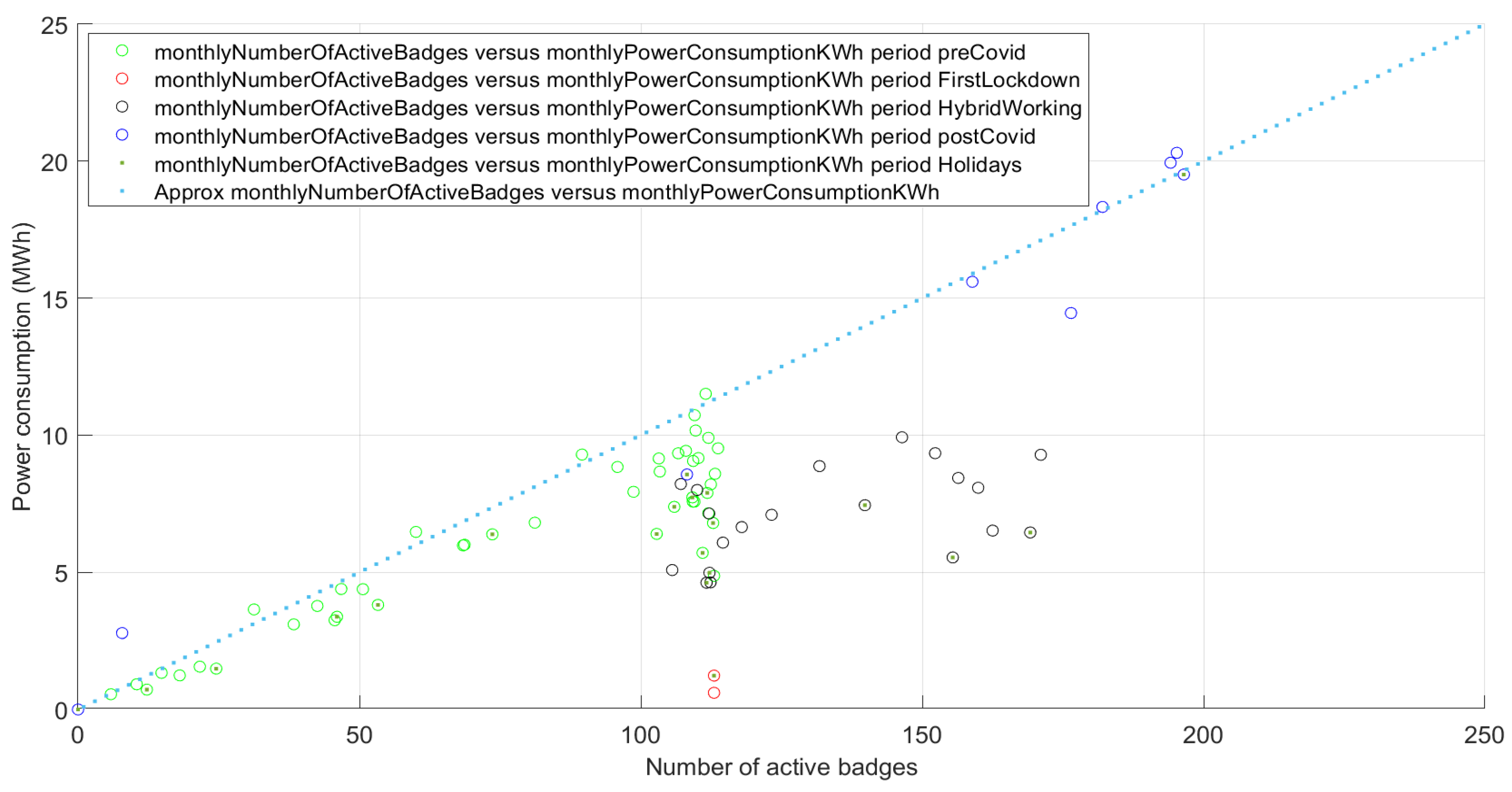
4.2.5. Relationship 2: Active Badge versus Energy Consumption

Figure 8 illustrates the relationship between the monthly energy consumption (noted E m o n t h l y , in kWh) and the number of active badges (noted B m o n t h l y without units) during the same month. The colors used in Figure 8 represent the same periods in Figure 7. It can be observed that there exists a simple linear dependence (represented with a dotted line) between the number of active badges and the maximum monthly energy consumption. This dependency is expressed in the following formula, further referred to as the second relationship in our methodology:
E m o n t h l y k W h = 100 × B m o n t h l y

4.3. PV Production

4.3.1. Production and Forecast Profiles

The PV production forecast is based on public forecasts provided by the French TSO, RTE. This forecast is the aggregated French PV production. It is calculated on the morning (approximately at 8 o’clock) of the current day. The time step of the forecast is one hour. We have retrieved the forecast data for the considered period. It is represented in Figure 9 (left). As the installed PV capacity increased significantly in France during this period, we have corrected the values in order to obtain forecasts such that the installed capacity would have been constant. We also normalized these values in such a way that they correspond to the production of a plant with a given peak power. In Figure 9 (right), this peak power is equal to 1 kWp.
In order to eliminate the effect of forecast imprecision, we suppose that the CPO is able to perfectly forecast the PV production. Thus, forecasted data is considered as the PV production.

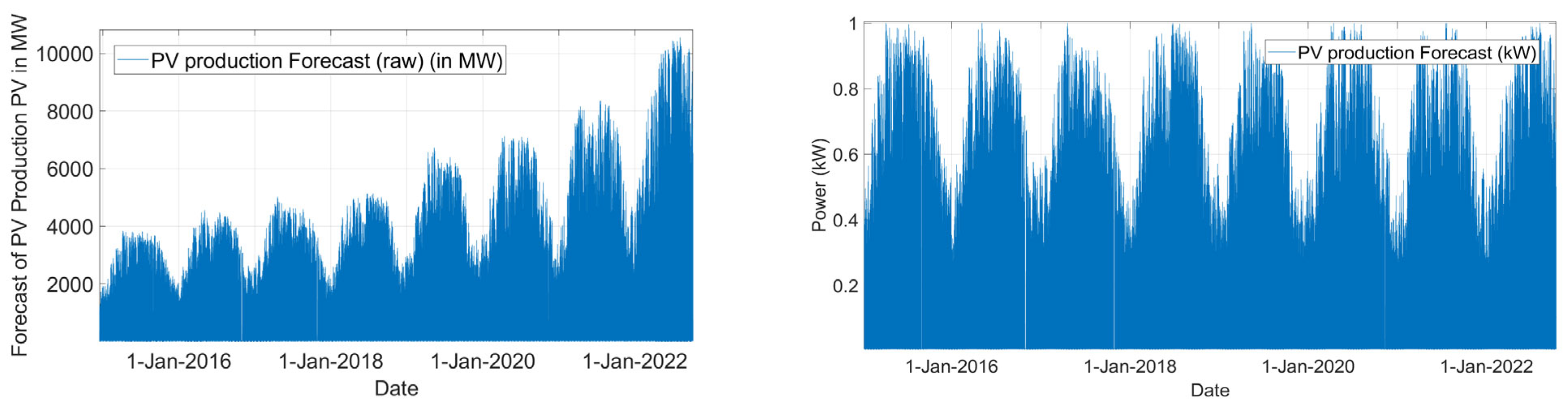
4.3.2. Relationship 3: Yearly PV Production versus Peak Power

There are two manners to obtain the yearly PV energy production from a peak power value for a given location as required to obtain the third relationship.
  • If production profiles are available, integrating the power over a complete year gives the energy produced during this year;
  • If production profiles are not available, many free software tools like PVGIS [28] estimate the annual PV production per peak power value.

4.4. Solar EV Charging

4.4.1. Production-to-Consumption Ratio

We have calculated the Production-to-Consumption ratio for annual periods (each begins on the 1st of June and ends on the 31st of May the next year) and for the period that begins on the 1 June 2021 and ends on the 31 August 2022. These values are summarized in Table 4, in which we can observe that the annual PV production is relatively constant while EV electricity consumption varies considerably.
It is also worth noting that the total production for the PV is rather large compared to the installed peak power (i.e., ~1.7 kWh per kW peak compared to ~1.6 kWh per kW peak estimated with PVGIS and with optimal orientation and tilt angle). This is because we have calculated the PV production from forecast data provided by RTE, and the normalization factor used for this aim has certainly been overestimated.

4.4.2. EV Charging Strategies

The charging power profiles for individual vehicles were not recorded during the period considered. Thus, we conduct simulations with different EV charging strategies based on charging session history to reconstruct these profiles. As the charging records contain the energy withdrawn by the vehicle i ( E i ) and the transaction duration DT, we suppose that this data are used by the CPO for controlling the charges. In practice, this data are not known, but they could be statistically estimated by the CPO. In this work, we consider three charging strategies with different complexity.
The first strategy is the Plug and Charge (PC) strategy described in Section 3.1. In that case, the charging power is limited by the nominal charging power of the embedded charger of the vehicle, noted P m a x i . The effective duration of the charging session is then equal to E i / P m a x i .
The second strategy is called ‘Mean Power’ (MP). In that case, the vehicle charges at constant power from the beginning to the end of the charging session. The duration of the charge is thus equal to DT and the constant charging power for vehicle i is E i / D T .
The third strategy is a Smart Charging (SC) strategy, whose main objective is to increase the self-production rate. The detailed algorithm is out of the scope of the article but can be briefly explained as follows. The PV production forecast of the PV plant is considered as the power that is “available” to charge the EVs. The planning algorithm then sorts the EVs according to the alphabetical order of the badges and allocates a part of this available power to each car. The principle of this allocation is as follows. The setpoints of a car are constituted of a constant power part added to a part that is proportional to the available power. Two constraints have been taken into account when choosing the setpoints: the sum of the power has to be less than the maximum power of the car ( P m a x i ) and the integrate of the setpoints has to be equal to the energy withdrawn by the car (   E i ).

4.4.3. Load Curve Reconstruction

Figure 10 represents the simulated load curves of 11 July 2018, obtained for different strategies and with a 75 kWp PV installation. The PV production is represented in blue. The curve that corresponds to the EV consumption with the PC strategy, in red, shows a large peak of approximately 200 kW at the beginning of the day and a second peak at noon. The curve that corresponds to the MP strategy, in yellow, is smoother and relatively synchronized with the PV production, but we observe that the EVs consume energy during the night (due to EVs that stay connected for more than a day). The curve that corresponds to the Smart Charging strategy, in purple, is in line with the PV production. We observe that there is no power consumption during night-time.
On this particular day, the Self-Consumption and Self-Production Rates are considerably higher for MP and SC strategies than the basic PC since their charging profiles are distributed throughout the day, in particular, when the PV production is the highest. Thus, the SPR is equal to 49% with the PC strategy, 89% with the MP and 100% with the PC strategy. The SCR is equal to 31% with the PC strategy, 62% with the MP and 69% with the PC strategy.

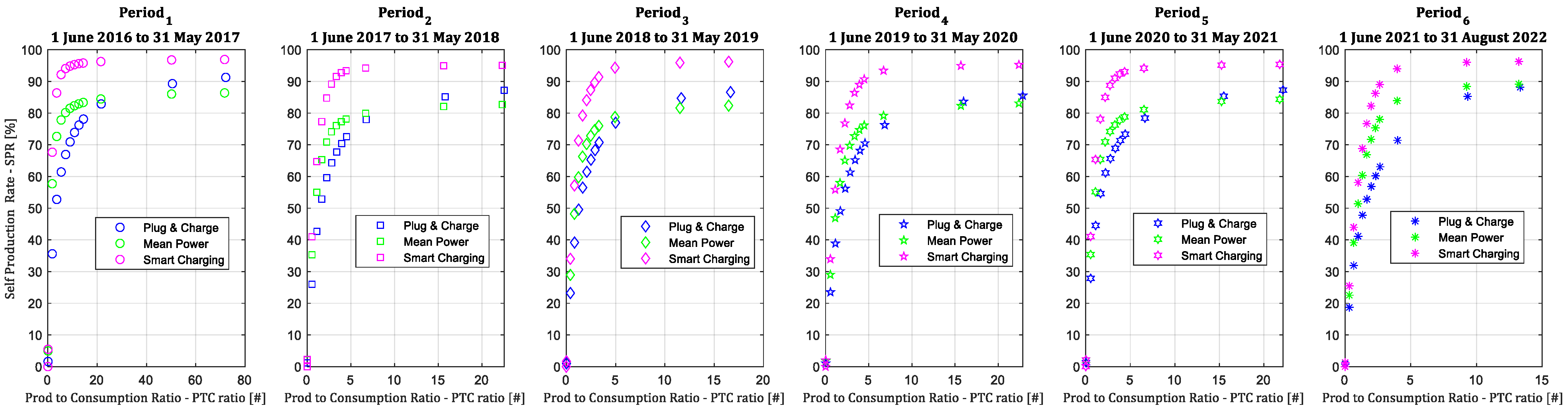
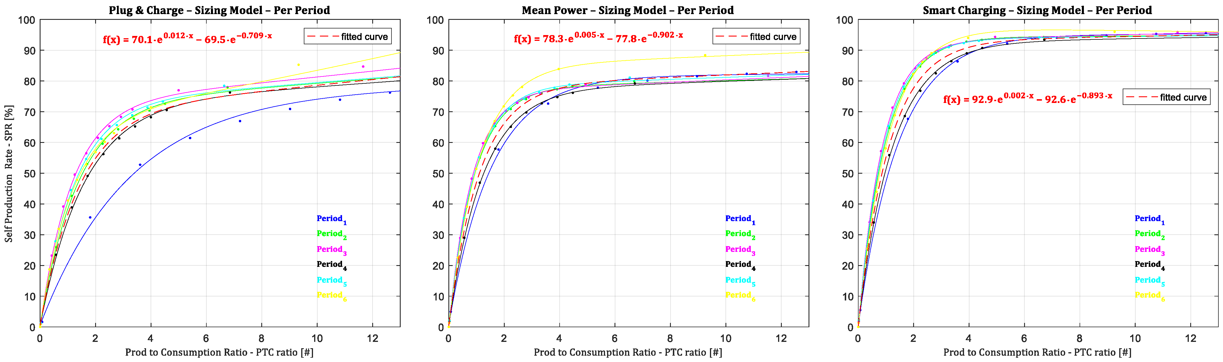
4.4.4. Relationship 4: Production-to-Consumption Ratio versus and Self-Production Rate

This section explores the relationship between the Production-to-Consumption ratio (PTC) and the SPR, given a particular charging strategy chosen among the three described in Section 4.4.2. In order to vary the PTC, as the total energy consumption of the cars is independent of the charging strategy, we have modified the value of the PV production. Fifteen different sizes of the PV plant have been considered for this study: Speak = [0, 1, 25, 50, 75, 100, 125, 150, 175, 200, 300, 700, 1000, 5000, 12,000] kWp.
First, we perform the following 17 simulations with the horizon spanning more than a 6-year period:
  • One simulation of the Plug and Charge strategy;
  • One simulation of the Mean Power strategy;
  • One simulation Smart charging strategy for each of the 15 different values of Speak.
Daily PTC and SPR for each of these simulations and for each value of PV plant size are then calculated. Figure 11 illustrates the values of daily PTC along with daily SPR, computed for a peak power value of 100 kWp, using more than 6 years of data. This figure distinguishes between the different charging strategies: in yellow, the results with smart charging, in red with Mean Power and in blue with Plug and Charge. We observe that the SPR is the highest for the smart charging strategy and is the lowest for the Plug and Charge strategy. We also observe that very high values of SPR are obtained with the SC strategy as soon as the PTC is higher than 1.
In addition, we have computed the PTC and SPR over the entire 6-year long period. Each point of Figure 12 has PTC as x-coordinates and SPR as y-coordinates. For the purpose of simplicity, only the PTC values obtained with the 10 lowest PV peak power values {0, 1, 25, 50, 75, 100, 125, 150, 175, 200} are displayed. The colors of the points distinguish different strategies similar to those in Figure 11.
We observe that, for a given value of PTC, the self-production increases with the SC strategy compared with the MP strategy. In the same way, the SPR increases with the MP strategy compared to the PC strategy. For example, for PTC = 1, the SPR is equal to 56% for the SC strategy, is equal to 48% for the MP strategy and is equal to 38% for the PC strategy. We can also observe that in order to obtain an SPR of 70%, the PTC has to be equal to 1.5 with the SC strategy, to 2.5 with the MP and to 4.1 with the PC strategy.
Notice that the results presented in Figure 12 allow us to simplistically aggregate our dataset and chosen strategies into the computational procedure described in Section 3.4.2. Such a choice is discussed in Section 5.2. The following subsection exemplifies the importance of these results in a specific use-case.

5. Sizing Procedure Examples

5.1. Price Examples

Since there are several stakeholders participating in the collective self-consumption scheme, the electricity would be billed differently according to stakeholder interactions. As assumed in Section 4.1.1, these bills are computed with flat rates and the cost of the electricity subscription is not considered.
The price of the electricity coming from the grid in this example is calculated by the Energy Regulation Commission (CRE) in France for 2023 [29]. The price structure of P r E S E V C P O   (424 €/MWh in total) is then composed of:
  • Energy Component: 322 €/MWh corresponding to “non-residential blue” tariff (version B, power subscription less than 36 kVA, included transportation, “supplementary power case” also called ‘alloproduit’ in french), as described in Annex B2 of [29];
  • Contribution Component: 31 €/MWh corresponding to the electricity consumption tax (Taxe Intérieure sur la Consommation Finale d’Electricité) or TICFE until 31 January 2022. This contribution since then has been reduced to 1 €/MWh as a result of electricity subsidy for French consumers (called “bouclier tarifaire” in french). Such a subsidy lasts until the end of 2024;
  • Tax Component: 71 €/MWh corresponding to 20% of the VAT on the energy, transport and contribution parts.
PV fit-in-tariff is a selling price also regulated by the CRE and is currently at 120 €/MWh (Tariff Tc, 100 kWp < P p e a k < 500 kWp in 2023) [30]. The purchase price P r P V O L P = P r P V O E S P V is thus supposed to be equal to 120 €/MWh as well. We consider that LP sells this energy at this price (i.e., without margin) but increased with transport, contribution and taxes. The price structure of P r L P C P O (197 €/MWh in total) is as follows:
  • Energy component: P r P V O L P = 120 €/MWh;
  • Transportation component: 13 €/MWh (as explained in [31]);
  • Contribution part: 31 €/MWh corresponding to TICFE;
  • Tax Component: 33 €/MWh corresponding to 20% of the VAT on the energy, transport and contribution.
A summary of these prices’ structure described above is given in Table 5.

5.2. Hypothesis

In the following examples, we suppose that the CPO plans to apply the methodology for prefeasibility studies (i.e., with the lowest effort but at the price of relatively low precision). Its use-case has to be similar to the one described in this paper in order to utilize the integrated dataset of the fourth relationship. In particular:
  • The configuration of the charging points must be similar to the one presented in Section 3.1, i.e., 100% of the charging points are 22 kW AC;
  • The characteristics of the EVs are identical to the presented ones (i.e., a probability distribution similar to the one of Figure 6);
  • The working time and user behavior (i.e., the statistics of the start and end date of the transaction, as depicted in Figure 4) are comparable;
  • The EVCI has to be large enough to integrate new users such that there is no congestion in the charging stations.
Note that if these assumptions are not satisfied, the fourth relationship is not valid and all the simulations would have to be performed again.

5.3. Sizing PV Given a Targeted Number of EVs and a Targeted Mean Power Price

As an illustration, let us consider that the CEA applies the method of this paper to size a PV plant located at Cadarache (near Aix-En-Provence, France) in order to charge its EV fleet in 2030. By using Figure 5, CEA observes that the number of EVs currently increases by approximately 100 per year. Thus, the number of EVs is assumed to be 1000 in 2030 (instead of 200 in 2022). By using Equation (8), this represents an annual consumption of 12 × 100 × 1000 = 1.2 GWh.
Let us consider that the CPO has a target price of P r C P O = 265 €/MWh. Equation (7) gives S P R = P r C P O P r E S E V C P O P r C P O L P P r E S E V C P O 70 % . Thanks to Figure 12, we identify that, in order to obtain an SPR of 70%, the ratio PTC has to be equal to 1.5, 2.5 and 4 for SC, MP and PC strategies, respectively.
With an EV consumption of 1.2 GWh, these correspond to an annual PV production of 1.8, 3 and 4.8 GWh. Once the required annual PV production has been identified, the PV peak power can be determined using solar potential for a particular location. For example, it is estimated that the PV production is about 1.4 GWh/MWp at the location of the experiment (south orientation, tilt angle of 20° and system loss of 18%). With such hypotheses, the peak power of the PV plant has to be equal to 1.28, 2.14 and 3.42 MWp to reach the targeted P r C P O L P .

5.4. Estimating the Mean Power Price Given an Existing PV Installation and a Number of EVs

Let us now suppose that the owner of an existing PV installation of 100 kWp in the same region wants to estimate the Mean Power price of the energy needed to feed 100 EVs with the smart charging strategy. The procedure for deriving this price, according to Figure 3, is the following:
  • From PVGIS: Annual PV Production E P V = 100 k W p × 1.4 M W h k W p = 140   M W h ;
  • From Equation (8): Annual EV Charging Consumption E E V = 12 × 100 k W h b a d g e × 100 [ b a d g e ] = 120 MWh;
  • Production-to-Consumption ratio P T C = E P V / E E V = 1 .16;
  • Self-Production Ratio (for Smart Charging) according to Figure 12: SPR = 0.6;
  • P r C P O can then be estimated from Equation (6);
  • P r C P O = P r E S E V C P O S P R P r E S E V C P O P r L P C P O 287   / M W h ;

5.5. Estimating the Number of EVs Given an Existing PV Installation and a Target Mean Power Price

Let us now suppose that the owner of an existing PV installation of 100 kWp in the same region wants to determine the number of EVs that it could charge with the Mean Power strategy and with a targeted Mean Power price of P r C P O = 265 €/MWh. The procedure for deriving the number of EVs that it can support is as follows, according to Figure 3:
  • From PVGIS: Annual PV Production E P V = 100 k W p × 1.4 M W h k W p = 140   M W h ;
  • From Equation (7), S P R = P r C P O P r E S E V C P O P r C P O L P P r E S E V C P O = 265 424 197 424 0.7 ;
  • The Production-to-Consumption ratio for different strategies is determined using Figure 12: P T C M P = 2.5 ;
  • Annual EV Charging Consumption (using the MP strategy) is then E E V = E P V P T C = 140 M W h 2.5 = 56   M W h ;
  • From Equation (8), the optimal number of EVs is then: E E V 12 × 100 = 56   M W h 12 × 100   k W h 46 .

6. Conclusions and Perspectives

In this study, we proposed a method for:
  • Sizing the PV plant required to properly charge a certain number of EVs, given a targeted Mean Power price;
  • Estimating the Mean Power price, given a PV plant size and the number of EVs to be charged;
  • Estimating the number of chargeable EVs for a particular PV installation and charging price.
We have applied this method to a car park located in a research center in southern France. The main input of this study is a massive empirical dataset collected over more than 6 years with 350 EV users and 80 charging points. To generate the EV charging power profiles, simulations were conducted with different charging strategies based on historical real data. This allowed us to obtain simulated EV profiles for the individual power demand and for different sizes of the PV plant. The effect of implementing rule-based charging strategies (Mean Power and Solar Smart Charging) has been proven to be significantly beneficial as compared to the simple Plug and Charge mode. In one of the showcases, the PV peak power required for 1000 vehicles to attain a charging cost of 265 €/MWh for Smart Charging, Mean Power and Plug and Charge strategies are 1.28, 2.14 and 3.42 MWp, respectively.
The main advantage of our methodology is its modularity, i.e., each key parameter (PV production, EV charging demand, business models and EV charging strategies) may be analyzed independently from each other. Thus, when the method is fully applied once on a given case, some computations may be re-used for other “similar” cases. In some cases, as fully exemplified in the previous section, the application of the method becomes very simple and quick.
The described methodology and results offer several avenues for future expansion:
  • Different simple and advanced strategies can be further integrated into this methodology, among which optimization-based methods are the most promising, in particular, Mixed Integer Linear Programming (MILP);
  • More realistic electricity tariff schemes (time-of-use or dynamic spot price) should be considered instead of flat rates from the energy provider ESEV;
  • Costs due to power subscription (in €/MW) should also be taken into account, in addition to the total electricity consumption (in €/MWh) as the number of EVs grows;
  • This paper assumes that the PV forecast is perfectly precise and omits any negative impact on the PV forecast accuracy. Hence, further studies are required to determine the impact of real PV forecast;
  • Individual Battery Degradation should be considered [32].
In contrast, we think that datasets representative of standard use-cases could be openly disseminated within the research community, as suggested in [33]. Such datasets could serve as valuable resources for benchmarking purposes. Furthermore, with increasingly higher aggregated EV capacity, the EVCI is also eligible for different market participation, thus creating several revenue streams for the CPO. For example, two of these markets encompass the European frequency containment market and demand-response market.

Author Contributions

Conceptualization, B.R. and L.M.; Software, B.R. and M.-F.B.; Validation, B.R. and V.-L.N.; Investigation, L.M.; Resources, B.R.; Data curation, B.R., L.M. and M.-F.B.; Writing—original draft, B.R.; Writing—review & editing, B.R., V.-L.N., M.-F.B. and A.M.; Visualization, B.R., V.-L.N. and M.-F.B.; Project administration, A.M.; Funding acquisition, A.M. All authors have read and agreed to the published version of the manuscript.

Funding

This work was supported by ADEME France, project PV2E_Mobility (grant number #1905C0043) and project T-IPV (grant number #2308D0002) and by the French National Program “Programme d’Investissements d’Avenir-INES.2S” (grant number ANR-10-IEED-0014-01).

Institutional Review Board Statement

Not applicable.

Informed Consent Statement

Not applicable.

Data Availability Statement

Not applicable.

Acknowledgments

We would like to show our gratitude to the direction and the logistics department of CEA Cadarache. We also thank our colleagues from INES/CEA Grenoble who provided expertise for the software development. We would also like to express our gratitude to the anonymous reviewers for their fruitful comments.

Conflicts of Interest

The authors declare no conflict of interest.

Abbreviations

PVPhotovoltaic
EVElectric Vehicle
CPOCharging Point Operator
PVOPhotovoltaic Operator
DSODistribution System Operator
EVCIElectric Vehicle Charging Infrastructure
ESEVEnergy Supplier of Electric Vehicles
ESPVEnergy Supplier of Photovoltaics
FSFeasibility study
LPLegal Person (La Personne Morale)
PVCSPhotovoltaic-powered Electric Vehicle Charging Station
PTCProduction-to-Consumption Ratio
PFSPrefeasibility study
SPR/SCRSelf-Production/Consumption Ratio
BESBattery Energy storage System
WTWind Turbine

Appendix A

Appendix A.1. Analytical Expression of the Relationship 4

Relationship 4, discussed in Section 4.4.4, is obtained from simulation results and is represented as an abacus. However, using the abacus directly is impractical due to the need for more automation in determining SPR from the PTC ratio (and vice-versa). Additionally, the points on the abacus are widely spaced, posing challenges for users trying to obtain one value given another. We propose utilizing analytical functions that interpolate between the abacus points to address these limitations. These functions can be integrated into software as mathematical expressions or lookup tables. To achieve this, we used the Matlab Curve Fitting ToolboxTM. Based on this analysis, the best-fit model for the data in Figure 12 is a two-term exponential function, which can be defined using the specific coefficients in Table A1.
Table A1. Coefficients of the analytical expression.
StrategyAnalytical Formula
Plug and Charge: S P R P T C = 70.1 × e 0.012 × P T C 69.5 × e 0.709 × P T C
Mean Power: S P R P T C = 78.3 × e 0.005 × P T C 77.8 × e 0.902 × P T C
Smart Charging: S P R P T C = 92.9 × e 0.002 × P T C 92.6 × e 0.893 × P T C
Figure A1 presents the points of the abacus and the associated analytical functions for the three control strategies.
Figure A1. Self Production Rate (SPR) as a Function of Production-to-Consumption (PTC) Ratio for over Six Years, Illustrated for Three strategies.
Applsci 13 10128 g0a1
We generated a look-up table using the derived analytical formulas to compute PTC ratios based on SPR input. Figure A2 illustrates the results for the three strategies, including an example of PTC ratios for an SPR of 70% (which is the value targeted in the sizing example of 5.3). Among the strategies, Smart Charging achieved the best ratio (PTC = 1.6), outperforming Mean Power (PTC = 2.4) and Plug and Charge (PTC = 4.2).
Figure A2. Production-to-Consumption (PTC) Ratio as a Function of Self Production Rate (SPR) for the 6-year period and for the three strategies.
Applsci 13 10128 g0a2

Appendix A.2. Sensitivity Analysis

Based on the six defined periods in Table 4, we computed the SPR and PTC, resulting in six abacus diagrams shown below (Figure A3). Each sub-figure represents SPR versus PTC for the three strategies: Plug and Charge (blue), Mean Power (green), and Smart Charging (magenta). In the first period (June 2016 to May 2017), PTC ranges from 0 to 80; in the last period (from June 2021 to August 2022), PTC ranges from 0 to 15. This variation is due to similar PV production during both periods but a significant increase in EV consumption.
Figure A3. SPR versus PTC ratio calculated for each of the six periods and for the three strategies.
Applsci 13 10128 g0a3
We applied the same curve fitting method to the six periods, resulting in curves represented in different colors. Figure A4 shows the curves for each period: blue (starting June 2016), green (starting 1 June 2017), pink (starting 1 June 2018), black (starting 1 June 2019), cyan (starting 1 June 2020), and yellow (starting 1 June 2021). The dotted red line also represents the curve obtained for the entire period.
Figure A4. Fitting Functions Comparison for six periods and the entire period.
Applsci 13 10128 g0a4
We notice that all the curves are nearly identical except for the curve associated with the first period and the Plug and Charge strategy (blue in the left sub-figure). The former curve is noticeably lower than the others, indicating that the SPR during that period was lower compared to the other periods for a given PTC. This can be attributed to the scarcity of EVs during that time (less than 50, according to Figure 5), with a higher proportion of them charging early in the morning. Furthermore, we observe that the curves calculated over the period of more than six years are consistently below those for period 2, period 3, period 4, and period 5. This suggests that the SPR estimated by relationship 4 is slightly pessimistic compared to the SPR observed during these four periods. In other words, our methodology, as described in Section 3.4, tends to oversize the PV peak power, overestimate the Mean Power price, and underestimate the value of EVs.

References

  1. Légifrance. LOI n° 2023-175 du 10 Mars 2023 Relative à L’accéleration de la Production D’énergies Renouvelables. Available online: https://www.legifrance.gouv.fr/dossierlegislatif/JORFDOLE000046329719/ (accessed on 23 May 2023).
  2. Hoarau, Q.; Perez, Y. Interactions between electric mobility and photovoltaic generation: A review. Renew. Sustain. Energy Rev. 2018, 94, 510–522. [Google Scholar] [CrossRef]
  3. Bhatti, A.R.; Salam, Z.; Aziz, M.J.B.A.; Yee, K.P. A critical review of electric vehicle charging using solar photovoltaic. Int. J. Energy Res. 2015, 40, 439–461. [Google Scholar] [CrossRef]
  4. Liu, L.; Kong, F.; Liu, X.; Peng, Y.; Wang, Q. A review on electric vehicles interacting with renewable energy in smart grid. Renew. Sustain. Energy Rev. 2015, 51, 648–661. [Google Scholar] [CrossRef]
  5. Nunes, P.; Figueiredo, R.; Brito, M.C. The use of parking lots to solar-charge electric vehicles. Renew. Sustain. Energy Rev. 2016, 66, 679–693. [Google Scholar] [CrossRef]
  6. Merten, J.; Guillou, H.; Ha, L.; Quenard, M.; Wiss, O.; Barruel, F. Solar Mobility: Two Years of Practical Experience Charging Ten Cars with Solar Energy. In Proceedings of the 5th International Conference on Integration of Renewable and Distributed Energy Resources, Berlin, Germany, 4 December 2012. [Google Scholar]
  7. Robisson, B.; Guillemin, S.; Marchadier, L.; Vignal, G.; Mignonac, A. Solar Charging of Electric Vehicles: Experimental Results. Appl. Sci. 2022, 12, 4523. [Google Scholar] [CrossRef]
  8. Danish Energy Agency. Prefeasibility Studies Guidelines-Methodology Overview on How to Conduct a Preseasibility Assessment of Renewable Power Generation Technologies. Available online: https://ens.dk/sites/ens.dk/files/Globalcooperation/prefeasibility_study_guidelines_final.pdf (accessed on 31 August 2023).
  9. Vermeer, W.; Mouli, G.R.C.; Bauer, P. Optimal Sizing and Control of a PV-EV-BES Charging System Including Primary Frequency Control and Component Degradation. IEEE Open J. Ind. Electron. Soc. 2022, 3, 236–251. [Google Scholar] [CrossRef]
  10. Figueiredo, R.; Nunes, P.; Brito, M.C. The feasibility of solar parking lots for electric vehicles. Energy 2017, 140, 1182–1197. [Google Scholar] [CrossRef]
  11. Al-Ogaili, A.S.; Hashim, T.J.T.; Rahmat, N.A.; Ramasamy, A.K.; Marsadek, M.B.; Faisal, M.; Hannan, M.A. Review on Scheduling, Clustering, and Forecasting Strategies for Controlling Electric Vehicle Charging: Challenges and Recommendations. IEEE Access 2019, 7, 128353–128371. [Google Scholar] [CrossRef]
  12. Latimier, R.L.G.; Kovaltchouk, T.; Ben Ahmed, H.; Multon, B. Preliminary sizing of a collaborative system: Photovoltaic power plant and electric vehicle fleet. In Proceedings of the 2014 Ninth International Conference on Ecological Vehicles and Renewable Energies (EVER), Monte-Carlo, Monaco, 25 March 2014. [Google Scholar] [CrossRef]
  13. GAMS: The General Algebraic Modeling System. Available online: https://www.gams.com/ (accessed on 31 August 2023).
  14. Atia, R.; Yamada, N. Sizing and Analysis of Renewable Energy and Battery Systems in Residential Microgrids. IEEE Trans. Smart Grid 2016, 7, 1204–1213. [Google Scholar] [CrossRef]
  15. IBM CPLEX Optimizer. Available online: https://www.ibm.com/fr-fr/analytics/cplex-optimizer (accessed on 31 August 2023).
  16. Naghibi, B.; Masoum, M.A.S.; Deilami, S. Effects of V2H Integration on Optimal Sizing of Renewable Resources in Smart Home Based on Monte Carlo Simulations. IEEE Power Energy Technol. Syst. J. 2018, 5, 73–84. [Google Scholar] [CrossRef]
  17. Sedighizadeh, D.; Masehian, E. Particle Swarm Optimization Methods, Taxonomy and Applications. Int. J. Comput. Theory Eng. 2009, 1, 486–502. [Google Scholar] [CrossRef]
  18. Chandra, G.R.; Bauer, P.; Zeman, M. System design for a solar powered electric vehicle charging station for workplaces. Appl. Energy 2016, 168, 434–443. [Google Scholar] [CrossRef]
  19. Tulpule, P.; Marano, V.; Yurkovich, S.; Rizzoni, G. Energy economic analysis of PV based charging station at workplace parking garage. In Proceedings of the IEEE 2011 Energy Tech, Cleveland, OH, USA, 25–26 May 2011. [Google Scholar] [CrossRef]
  20. MathWorks. Available online: https://fr.mathworks.com/ (accessed on 31 August 2023).
  21. NREL System Advisor Model (SAM). Available online: https://sam.nrel.gov (accessed on 12 June 2018).
  22. Tulpule, P.J.; Marano, V.; Yurkovich, S.; Rizzoni, G. Economic and environmental impacts of a PV powered workplace parking garage charging station. Appl. Energy 2013, 108, 323–332. [Google Scholar] [CrossRef]
  23. Yan, D.; Ma, C. Optimal Sizing of A PV Based Electric Vehicle Charging Station under Uncertainties. In Proceedings of the IECON 2019-45th Annual Conference of the IEEE Industrial Electronics Society, Lisbon, Portugal, 14–17 October 2019. [Google Scholar] [CrossRef]
  24. Krim, Y.; Sechilariu, M.; Locment, F. PV Benefits Assessment for PV-Powered Charging Stations for Electric Vehicles. Appl. Sci. 2021, 11, 4127. [Google Scholar] [CrossRef]
  25. Roselli, C.; Sasso, M. Integration between electric vehicle charging and PV system to increase self-consumption of an office application. Energy Convers. Manag. 2016, 130, 130–140. [Google Scholar] [CrossRef]
  26. Ritte, L.-M.; Mischinger, S.; Strunz, K.; Eckstein, J. Modeling photovoltaic optimized charging of electric vehicles. In Proceedings of the 3rd IEEE PES Innovative Smart Grid Technologies Europe (ISGT Europe), Berlin, Germany, 14–17 October 2012. [Google Scholar]
  27. Mischinger, S.; Strunz, K.; Eckstein, J. Modeling and evaluation of battery electric vehicle usage by commuters. In Proceedings of the IEEE Power and Energy Society General Meeting, Detroit, MI, USA, 24–28 July 2011. [Google Scholar]
  28. European Commission. Photovoltaic Geographical Information System. Available online: https://re.jrc.ec.europa.eu/pvg_tools/fr/ (accessed on 3 July 2023).
  29. Wargon, E.; Cellier, A.; Edwige, C.; Faucheux, I.; Plagnol, V. Délibération de la CRE du 19 Janvier 2023 Portant Proposition Des tarifs Réglementés de Vente D’électricité. Available online: https://www.cre.fr/Documents/Deliberations/Proposition/proposition-des-tarifs-reglementes-de-vente-d-electricite-1er-fevrier-2023 (accessed on 19 January 2023).
  30. Wargon, E.; Edwige, C.; Faucheux, I. Délibération de la CRE du 12 Octobre 2022 Portant Avis sur le Projet D’arrêté Modifiant L’arrêté du 6 Octobre 2021 Fixant Les Conditions D’achat de L’électricité Produite par les Installations Implantées sur Bâtiment, Hangar ou Ombrière Utilisant L’énergi. Available online: https://www.cre.fr/Documents/Deliberations/Avis/projet-d-arrete-modifiant-l-arrete-du-6-octobre-2021-fixant-les-conditions-d-achat-de-l-electricite-produite-par-les-installations-implantees-sur-b (accessed on 12 October 2022).
  31. Enedis. Le Tarif D’Acheminement de L’Électricité (TURPE). Available online: https://www.enedis.fr/le-tarif-dacheminement-de-lelectricite-turpe (accessed on 31 August 2023).
  32. Zheng, Y.; Shao, Z.; Lei, X.; Shi, Y.; Jian, L. The economic analysis of electric vehicle aggregators participating in energy and regulation markets considering battery degradation. J. Energy Storage 2021, 45, 103770. [Google Scholar] [CrossRef]
  33. Fachrizal, R.; Shepero, M.; van der Meer, D.; Munkhammar, J.; Widén, J. Smart charging of electric vehicles considering photovoltaic power production and electricity consumption: A review. eTransportation 2020, 4, 100056. [Google Scholar] [CrossRef]
Figure 1. Interactions of the EVCI’s stakeholders.
Applsci 13 10128 g001
Figure 2. Principle of collective self-consumption scheme.
Applsci 13 10128 g002
Figure 3. Computational procedure for EV and PV sizing.
Applsci 13 10128 g003
Figure 4. Histograms of start and end times of charging sessions.
Applsci 13 10128 g004
Figure 5. Number of active and delivered badges.
Applsci 13 10128 g005
Figure 6. Histograms of vehicles’ (a) nominal charging power and (b) battery capacity.
Applsci 13 10128 g006
Figure 7. Monthly energy consumption of the dataset.
Applsci 13 10128 g007
Figure 8. Monthly EV power consumption versus monthly number of active badges.
Applsci 13 10128 g008
Figure 9. Raw production forecast (left) and corrected values (right).
Applsci 13 10128 g009
Figure 10. Simulation results on 11th July 2018 for a PV system of 75 kWp.
Applsci 13 10128 g010
Figure 11. Daily SPR and Daily PTC for every day for 6 years of the experimentation.
Applsci 13 10128 g011
Figure 12. Relationship 4: PTC vs SPR, computed for different PV peak powers (0, 1, 25, 50, 75, 100, 125, 150, 175, 200) over a more than 6-year period.
Applsci 13 10128 g012
Table 2. Nomenclature of variables used in this paper.
SymbolExplanation
P E V Power supplied for EV Charging (kW)
P P V Power generated by PV (kW)
P E S E V Power extracted from the grid to charge EV (kW)
P E S P V Power injected to the grid from PV (kW)
P S P Power from PV for EV charging (kW)
E E V ,   P V ,   E S E V ,   E S P V , S P Δ Integration of the corresponding powers over certain duration ∆ (kWh)
P r P V O E S P V Purchasing price of EESPV by ESPV (€/MWh)
P r E S E V C P O Purchasing price for EESEV by CPO (€/MWh)
P r L P C P O Purchasing price for ESP by CPO (€/MWh)
P r C P O Mean power price for the CPO (€/MWh)
Table 3. Input and Output data.
Input
Output
Price
Network Power
P r E S E V C P O
Price PV Power
P r E S P V C P O
Mean Power Price
P r C P O
PV
Potential
PV Peak Power
P P V p e a k
# EV
Users
EVs
Characteristics
Charging Session
History
Badge/EV Model
Peak PowerXXXX XXXX
Mean Power PriceXX XXXXXX
#EV usersXXXXX XXX
Table 4. Sum-up of the PV production, the EV consumption and the PTC ratio over the 6-year period.
PeriodsDuration (Months)Annual PV Production (100 kWp)
MWh
Annual EV Consumption (MWh)Annual PTC Ratio
1 June 2016–31 May 201712178247.21
1 June 2017–31 May 201812171762.25
1 June 2018–31 May 2019121801091.66
1 June 2019–31 May 202012173762.28
1 June 2020–31 May 202112171772.21
1 June 2021–31 August 2022152381781.33
Table 5. Electricity Prices for different stakeholder interactions. Notice that these prices are simple flat rates.
InteractionNomenclaturePrices (€/MWh)Price Structure
PVO sells to LP P r P V O L P 120120 Energy
LP sells to CPO P r L P C P O 197120 Energy + 13 Transport + 64 (Taxes and contribution)
ESEV sells to CPO P r E S E V C P O 424322 (Energy + transport), 102 (Taxes and contributions)
Disclaimer/Publisher’s Note: The statements, opinions and data contained in all publications are solely those of the individual author(s) and contributor(s) and not of MDPI and/or the editor(s). MDPI and/or the editor(s) disclaim responsibility for any injury to people or property resulting from any ideas, methods, instructions or products referred to in the content.

