Abstract
With the increase in rooftop photovoltaic (PV) systems at the residential level, customers owning such renewable resources can act as a source of generation for other consumers in the same network. Peer-to-peer (P2P) energy trading refers to a local trading platform where the residential customers having excess PV power (prosumers) can interact with their neighbors without PV resources (customers) to improve the social welfare of society. However, the performance of a P2P market depends on the power system network constraints and trading strategy adopted for local energy trading. In this paper, we compare different trading strategies, i.e., the rule-based zero intelligent (ZI) strategy and the preference-based game theory (GT) approaches, for a constrained P2P platform. Quadratic trading loss and impedance-based network utilization fee models are suggested to define the network constraints for the P2P system. Additionally, a reluctance-based prosumer-sensitive model is developed to adjust the trading behavior of the participants under the heavy distribution losses/network fee. The presented results show that the suggested trading strategies enhanced the average welfare of the participants by approximately 17%. On average, the customers saved about $33.77 monthly, whereas the average monthly earnings of the prosumers were around $28.3. The ZI strategy enhanced the average monetary advantages of all the market participants by an average of 7% for a system having small distribution losses and a network fee as compared to the GT approach. Contrarily, for a system having high losses/a utilization fee, the GT approach improved the average welfare of the prosumers by around 75% compared to the ZI strategy. However, both trading strategies yielded competitive results compared to the traditional market under the standard values of network coefficients.
1. Introduction
Deregulated structures offer a competitive market environment where participating customers can interact autonomously to enhance their social welfare [1]. A peer-to-peer (P2P) structure is a local competitive market framework where customers with surplus energy produced by renewable power, such as photovoltaic (PV) solar or previously stored in a battery energy storage system (BESS) can sell it to the other consumers in the same network. These consumers with excess energy are known as prosumers in the P2P network. The basic intuition of the P2P platform is to efficiently utilize the PV energy of prosumers to improve the welfare of the P2P community. In traditional vertically aligned grids, the excess PV power can only be shared with the grid, which results in a limited flexibility for the prosumers. However, with the advancements in smart grids, the prosumers can interact with their neighbors to sell their PV energy at the desired price in the form of P2P trading. The main advantages of a P2P market are competitive buying/selling rates and increased flexibility for the market participants [2,3]. In P2P markets, prosumers can sell their PV energy at a competitive price compared to a utility feed-in tariff (FIT), whereas customers can meet their demand at a price that is lower than the utility price [4]. This sets up a competitive trading environment, where the participants can get competitive rates compared to the traditional market prices [5,6].
P2P markets can be set up using a centralized method, i.e., the energy transactions are monitored by a central entity such as the market operator or an aggregator, or using a decentralized method, i.e., the customers trade without any central operator overlooking the transactions [7,8]. The formulation of the P2P network depends on the bidding strategy used for the participants and the physical constraints of the network. The proper selection of the trading strategy can ensure a positive welfare for the P2P market by giving additional monetary advantages to the participants. Contrarily, if unaccounted for, the network constraints of the system can impair the welfare of the market. Different methods have been presented in the literature to model the behavior of such markets under the influence of the physical constraints of the network [9].
The major challenge for P2P platforms is to decide the optimal type of trading strategy based on the network parameters of the system. An improper selection of the bidding framework can impair the performance of the P2P platform under varying network parameters [10]. In this paper, we provide a comparison of two different trading strategies for the P2P platform while incorporating the network parameters and their impacts on the social–economic welfare of the market. Additionally, the reluctance-based sensitivity of prosumers towards the network parameters was developed to adjust the trading strategy of the participants based on the system parameters.
1.1. Literature Review
A literature survey of the P2P platforms with various bidding methods has been presented in this part of the introduction. Additionally, the importance of the network constraints for P2P markets has been shown from the previous literature.
1.1.1. Trading Strategies for P2P Platforms
One of the main components of P2P trading is the type of trading mechanism used for sharing PV energy between the prosumers and the customers. Different bidding strategies have been presented in the literature for P2P trading. In [11], a continuous double auction (CDA)-based market framework was formulated while using trading mechanisms such as the eyes on best (EOB) price and the zero intelligent (ZI) strategy. A privacy-preserved trading platform for the P2P market was developed in [12] for urban community microgrids while using the CDA mechanism. The authors in [12] proposed a price-targeting mechanism to maximize the profit of the participants in a decentralized manner. A nonuniform clearing mechanism using the k-continuous double auctions for the CDA-based structures was presented in [13] to optimally decide the clearing price based on the market behavior. The presented modification to the CDA trading mechanism in [13] resulted in a market-dependent clearing price to ensure maximum welfare for the customers. A robust trading price mechanism that considered the preference of the prosumers was suggested in [14] to develop the P2P structure within the microgrid. A dynamic price mechanism to find the equilibrium point between the traded quantity and the buy/sell price has been suggested in [15] for a smart community having renewable energy resources.
A blockchain-based implementation for the CDA markets was suggested in [16] using a game theory (GT) approach to optimally decide the clearing price for the customers. Similarly, the authors in [17] developed a decentralized GT pricing mechanism to solve the P2P trading problem in an energy blockchain environment to optimize the welfare of the prosumers in the microgrid. Various trading strategies such as uniform k-DA, discriminatory k-DA, Vickrey–Clark–Groves, and trade reduction auction mechanisms were compared in [18] for solar-based P2P trading platforms. The authors in [18] compared the bidding strategies under varying penetrations of PV energy resources for a suggested transactive energy framework. A cooperative GT-based approach was presented in [19] for a local energy community framework for maximizing the social welfare of both the customers and prosumers. A dual bidding strategy considering both inter- and intracommunity trading was suggested in [20] to enhance the economic welfare of the market participants while considering the uncertainties in the renewable power generation.
The mentioned literature survey covers the most commonly used trading strategies for the P2P platform. However, in the majority of the literature above, the network constraints were not considered while modeling the P2P trading structure. The energy transactions between the customers of a P2P market take place over the physical distribution lines of the utility, which are prone to trading losses. Similarly, the majority of implementations of P2P environments require a central entity to coordinate the transactions between participants. This requires a certain transaction fee for each P2P order for the market services provided by the market operator. The next part of the introduction provides an overview of the various implementations of P2P networks while considering network parameters.
1.1.2. P2P Market with Network Constraints
Network constraints play a pivotal role in determining the performance of a P2P market. The authors in [21] suggested network constraints for the P2P market in the form of trading losses and a network utilization fee. However, their implementation was limited to a social welfare maximization, and the individual welfare of each customer was not modeled using the network parameters. A constrained CDA market was developed in [22] for low-voltage (LV) networks using power factor distribution and loss factors for the network. A distribution locational marginal pricing (DLMP)-based formulation for the P2P networks was developed in [23] while developing the optimal-power-flow-based formulation for the LV networks.
A similar formulation for the P2P markets using the DLMP approach was suggested in [24] for a transactive energy framework for distribution networks. Trading losses have been suggested for the auction-based markets using the Bayesian GT in [25] to model the physical constraints for the P2P network. A DSO-based P2P market was formulated in [26] to model the interactions between the participants using the reserve constraints for the energy transactions. A congestion management for the LV P2P networks was suggested in [27] using the marginal prices of the network. The formulation in [28] models the individual behaviors of the market players of the P2P platform by using the user-centric behavior models while developing the network constraints for the P2P market. However, the implementation in [28] did not consider the optimal P2P clearance for the participants and the sensitivity of the prosumers towards the network coefficients.
1.2. Research Gaps and Contributions
The welfare of a P2P network depends on the type of bidding strategy and the physical parameters of the system. In a majority of the literature, (i) the network parameters are not considered while comparing the bidding mechanisms for the P2P participants; (ii) different trading strategies have not been explored while developing the constrained P2P markets; and (iii) the sensitivity of the prosumers towards the network parameters have not been discussed for modeling their trading behavior. Considering the mentioned research gaps, the proposed contributions are as follows:
- We modeled the intermittent nature of the PV sources for P2P trading prosumers using the fractional integral polynomial method;
- We compared different trading strategies, such as the rule-based ZI mechanism and GT approach, for constrained CDA markets for trading the PV energy to analyze the impact on the individual/social welfare;
- We suggested quadratic trading loss and network-impedance-based utilization fee models for the P2P markets to incorporate the network constraints;
- We designed a reluctance-based sensitivity model for the prosumers towards the network constraints of the system to highlight the trading pattern of the participants under heavy distribution losses/a network fee;
- We extended the P2P platform presented in [28] to incorporate the GT approach while considering the preference of the individuals and a sensitivity analysis of network parameters.
The remaining paper is organized as follows: Section 2 describes the system model for the suggested P2P market. In Section 3, the details of the market structure are presented. The results and analysis for the given test cases are discussed in Section 4. The findings of this research are concluded in Section 5.
2. System Model
The suggested model simulates the P2P market over the duration of a single day that is divided into number of intervals of equal duration . Additionally, the network consists of sets of prosumers and sets of customers trading with each other such that . Note that in all of our discussion, we refer to customers as the participants that consume the PV energy of the prosumers.
The suggested framework consists of three stages, as shown in Figure 1. The first stage collects the input data (i.e., the load profiles, PV curves of the prosumers, and day-ahead market price). The second stage uses the data from the first stage to compute the winners and the market price range for each time interval using the CDA market. The bid signals refer to the price set up by the customers, whereas the ask values refer the market price set up by the prosumer. Finally, in the third stage, the market operator determines the optimal set of parameters (i.e., the optimal trading quantity and P2P price for the matched orders using the trading approach).
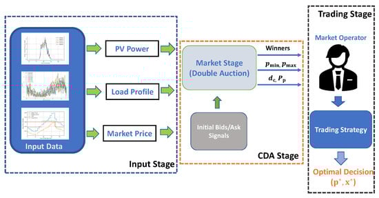
Figure 1.
Breakdown of different stages for the suggested market structure. The first step is to collect the input data for the CDA market. The second stage uses the CDA market to generate the winners for CDA auction. Third stage involves the trading strategy based on the parameters of the second stage to determine the optimal trading power and P2P price for each matched order.
Any unmatched orders at the end of P2P trading will be cleared at the utility price by the market operator. Prosumers will sell any excess renewable power as a FIT to the market operator. Similarly, the customers will pay the utility price to the market operator for meeting their demand.
2.1. Load Modeling for Market Participants
Load modeling is a crucial component for determining the demand curves of the P2P participants. This research uses the queuing load model as suggested in [29,30] to determine the load profile of the P2P participants. The queuing load model has the following advantages:
- The start time of each device is modeled as the output of a random process to capture the individual behavior of each participant. Due to the fact that the residential customers have distinct consumption patterns, queuing theory captures this uniqueness by determining the start time of each device randomly while still following a known stochastic process.
- To capture the daily and seasonal variations, the arrival rate of the devices are modeled using a Poisson distribution to capture the time-varying nature of the load.
While using the queuing theory, it is assumed that the population size and queue lengths are infinite to capture all the electric loads arriving into the queue. The model used in this research is an queue implement load model [31], where represents the Poisson process, G represents the probability distribution of the appliances, and ∞ indicates the infinite queue length. The Poisson process, , can then be defined mathematically as follows:
where and are the expected values for the duration and power of the electric loads for the market participant d, respectively. The individual load for each household can be modeled based on the aggregated distribution data as follows:
where and are the scaling coefficients for the individual household. The authors have provided a brief introduction of the suggested model for the simplicity of the readers. Further mathematical details and the analysis of the suggested queuing model are presented in [29,30].
2.2. Prosumer PV System Modeling
As the P2P trading model relies on excess prosumer energy, a prerequisite for the P2P platform is to model the PV curves for prosumers. This research uses the fractional integral polynomial method as suggested in [32] to model the PV energy of the prosumers by taking into account the following advantages:
- The suggested model uses parameters such as irradiance and temperature to find the PV energy, which reduces the modeling error compared to the standard irradiance-based models;
- The suggested model depends on manufacturer parameters such as the maximum voltage, temperature coefficient, short circuit current, and voltage coefficients. This models a practical P2P community, where each prosumer has a different PV system with distinct module parameters.
The subsequent subsections introduce the fractional integral polynomial method for modeling the PV power based on the characteristics of the module. First, the mathematical details of the model are presented based on the module parameters. The effect of the atmospheric parameters on the power of the PV system is then depicted by varying both the temperature and irradiance parameters. This models the intermittent nature of the PV system, which is imperative to set up any P2P trading platform.
2.2.1. Fractional Integral Polynomial Method
The suggested fractional integral model calculates the PV module as a function of the voltage, which is given as follows:
where and are the short circuit current and open circuit voltage parameters, respectively. Additionally, i represents the module current in the range , u represents the voltage of the module in the range , and represents a value given in the range . is a non-negative integer value. The power of the PV module can be determined as follows:
The above equations depend on the following major parameters: , and the sum of . These parameters depend on the atmospheric conditions and the manufacturer characteristics. The following equations determine the values of , and the sum of :
where, and are the series and parallel connected modules, respectively. and represent the standard test conditions (STC) parameters, G and T represent the arbitrary irradiance and temperature values, respectively, represents the open circuit voltage temperature coefficient, represents the short circuit current temperature coefficient, and represent the voltage limits for the PV module, and and are the rated PV module parameters. The validation of the Equations (3)–(7) is presented in the following subsections by varying the model parameters. Additionally, for complete mathematical details and derivation of the presented model, the readers are encouraged to go through the analysis provided in [32].
2.2.2. Temperature Effect on PV Power of Prosumers
One of the key advantages of using the suggested model compared to standard irradiance-based models is that it takes into account the effect of the temperature and the PV module characteristics on the power of the module. To demonstrate the impact of the temperature on the power output at a fixed irradiance, we implement our model for the module characteristics taken from [32]. The effect of the temperature on the i–u characteristics and the power is given in Figure 2. As is evident from Figure 2a,b, the temperature parameter affects the maximum power of the module.
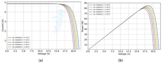
Figure 2.
Temperature effect on the characteristics of the PV module. (a) The i–u characteristics. (b) The power characteristics.
Figure 3 shows the effect of the temperature parameter for a PV system with a rated capacity of 5 kW and a system efficiency of 95% (the parameters for a single module are the same as those used for the results of Figure 2). From the figure, it is evident that the temperature parameter is important to model the PV curves for the prosumers. If unaccounted for, the modeling error for the given system was around 8%. The model using the irradiance parameter only ends up overestimating the PV power for the prosumer by around 0.32 kW, which, over a long-term market operation, would overestimate the prosumer energy available. Therefore, it is essential to use both the irradiance and temperature profiles of the prosumers for modeling the PV power for each P2P market interval. Note that any PV model that uses both the temperature and irradiance parameters (or standard irradiance-based models) for modeling the PV power can be used for the suggested P2P trading platform.
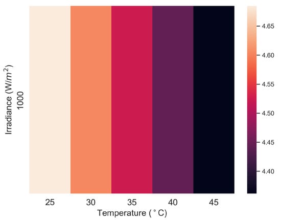
Figure 3.
Heat map for the power of the PV system for constant irradiance and varying temperature.
2.2.3. Irradiance Effect on PV Power of Prosumers
The suggested model was also validated for the same module characteristics as defined previously by varying the irradiance parameter while keeping temperature constant. Figure 4 shows the effect of the irradiance on the i–u and power characteristics of the module. From the given figure, it is evident that, by increasing the irradiance while keeping the temperature constant, this increased the maximum power of the module. Figure 5 shows the sensitivity of the PV system to both the irradiance and temperature parameters. The advantage of using the presented fractional integral model is its ability to model the intermittent nature of the PV system while using the atmospheric parameters, as depicted in Figure 2, Figure 3, Figure 4 and Figure 5.
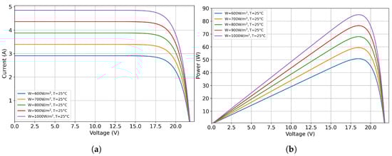
Figure 4.
Irradiance effect on the characteristics of the PV module. (a) The i-u characteristics. (b) The power characteristics.
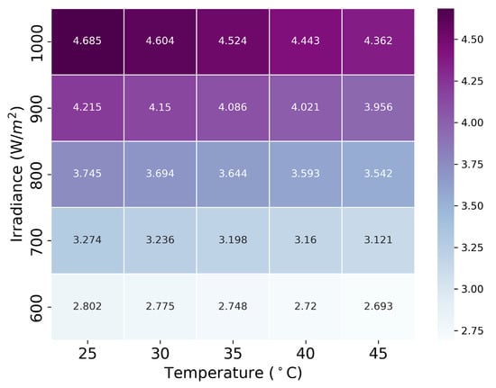
Figure 5.
Heat map for the power of the PV system for varying irradiance and temperature levels.
3. P2P Trading Platform
This section provides the details regarding the suggested P2P platform using different trading mechanisms under a CDA market structure while incorporating network constraints. The major steps involved are (i) setting up the initial bid/ask values, (ii) determining the winners of the market using an equilibrium-matching mechanism, (iii) computing the optimal set of quantities for each matched order using a bidding strategy, and (iv) designing a clearance mechanism. The details regarding different steps are given as follows:
3.1. Trading Strategies and Determination of Optimal Quantities
One of the fundamental steps for formulating a P2P platform is to develop the bidding mechanism for the market participants and to determine the optimal quantities for each P2P contract. This research compares two different strategies, i.e., the rule-based ZI method and the GT approach. The selected trading strategies are efficient in utilizing the energy of the prosumers in an intelligent fashion while increasing the monetary advantages of the market participants [11,18]. Additionally, the GT approach enables the participants to adjust their trading behavior based on the network parameters to avoid the negative welfare resulting from the system having high losses/a network fee. However, the presented framework can be implemented with any set of trading strategies. The quantities to determine the matched orders are the P2P price and the traded quantity. The next part of this section provides detailed description of the different trading mechanisms for the P2P platform, as well as the criterion used to determine the matched orders.
3.1.1. Strategy I: Rule-Based Zero Intelligent Strategy
The zero intelligent (ZI) strategy models the behavior of the market participants as “zero intelligent” by using a random criterion to generate the bid values. The main intuition behind using the ZI strategy is to generate the bid/ask signals within the limits of the utility values. The major advantage of using such a strategy is its constrained nature between the utility price and the FIT. Each prosumer will initialize the ask value, which cannot be higher than the utility tariff. Similarly, each customer will place a bid value that is greater than or equal to the FIT. This ensures a positive welfare for the participating customers/prosumers [11]. Mathematically, for any interval , the price signals generated using the ZI strategy are given as follows:
where and represent the bid and ask price of the ith customer, and jth prosumer, respectively, for the market interval, and are the FIT and retail values for the interval , respectively, and U represents a uniform random number in the range.
Figure 6 shows the initialization of the bids using the ZI strategy. From the figure, it is evident that the prosumers cannot put an ask price that is higher than the retail tariff. Similarly, the customers will initialize a bid value that is greater than the FIT. This ensures that, for the matched orders, the participants will get a better price compared to the utility value. After receiving the bid values for each customer, the next step is to use a matching mechanism for the proposed strategy. For finding the matched orders, equilibrium matching (EM) is proposed in this research.
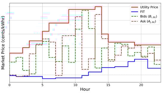
Figure 6.
Initialization of the bid/ask values using the ZI strategy.
- Equilibrium matching: EM sorts the bid values of the customers in descending order, whereas the ask prices for the prosumers are arranged in an ascending manner. P2P orders will be matched if the bid value is greater than or equal to the ask price [28]. This process will continue for all the P2P orders until the market interval terminates. Once the matched orders are determined using EM, the next part is to determine the trading price and quantity for each matched order.
- Determination of the price and traded quantity: Once an order is matched using EM, the rule-based ZI strategy determines the P2P price as follows:where represents the P2P price for the matched orders. The traded quantity can be determined based on the demand and the excess renewable power of the jth prosumer, which is defined as follows:where represents the traded quantity between ith customer and jth prosumer. Rule-based determination for the ZI strategy is a simple yet effective way of determining the optimal set of quantities for the matched contracts. However, it neglects the individual preference of the prosumers/customers towards determining the P2P price and amount of energy traded. This can impair the performance of the P2P network, especially under the constrained environment. The second strategy, a GT approach, provides an alternative to the simple rule-based determination to incorporate the individual preference of the market participants.
3.1.2. Strategy II: Preference-Based GT Approach
In the preference-based GT approach, the first step follows the rule-based determination, i.e., it determines the winners (matched orders) of the market using the EM approach. Consider a particular P2P order ; then, using the EM, the winners will be determined as follows:
where are the matched P2P contracts, and refer to the unmatched orders such that . refer to the total P2P contracts for a given market interval . For order , the quantities are given as follows:
The next step is to determine the optimal quantities for the matched contracts while considering the preference of the individuals.
Determination of and : For the orders , the quantities to find are the trading price and the trading quantity . This research uses a single-leader-, multiple-follower-based Stackelberg game (SLMFSG) approach to find the optimal quantities for the matched orders, as suggested in [33]. In our proposed framework, the market operator acts as a leader, and the market participants are the followers of the game that make their decisions based on the actions of the leader. For each , prosumer j computes the amount of power shared based on the utility function as follows:
where is the market trading price, is the excess renewable power, and is the reluctance parameter for the jth prosumer, respectively. The first part of the function is the revenue that the prosumer receives from sharing energy in the market. The reluctance term, , represents the negative impact on the utility of the prosumer j, which measures the unwillingness of the prosumer j to share its power in the P2P market [33]. For the given market price and the reluctance parameter , the objective of the prosumer is to maximize its utility function as follows:
In the SLMFSG approach, the leader (market operator) has no control over the decisions of the prosumers in solving its utility function. However, the operator sets the market price to consider the savings of the customers participating with the prosumers in P2P trading. The aim of the market operator is to choose the in such a way that it maximizes the cost savings of the customers, which are given as follows:
where represents the savings of the ith customer.
This forms an iterative process in which, at each iteration, the leader determines the market price while considering the savings of the customer based on the amount of energy shared . The prosumer will compute based on the to maximize its utility function (note that the solution to the objective function given in Equation (15) can be found using [33]) and sends the updated to the operator for the next iteration. This process continues until Stackelberg equilibrium is achieved. The pseudocode for the GT algorithm is given in Algorithm 1. The proof for the uniqueness of the Stackelberg solution for the given game can be found in [33]. Figure 7 shows the flowchart of the suggested P2P trading platform using both trading strategies.
| Algorithm 1 GT pseudocode for determining traded quantity and price |
| Input: and . in Output: . out Initialization: .
|
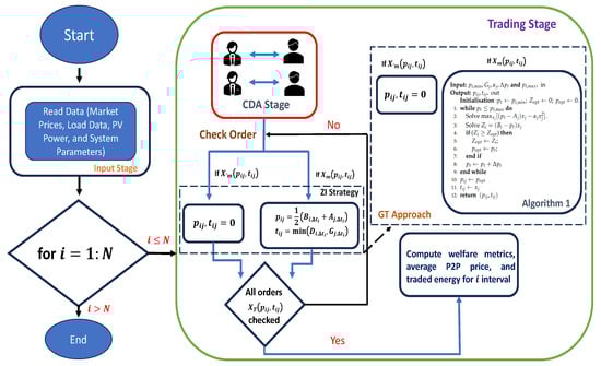
Figure 7.
Flow chart of the suggested trading strategies. First step involves collecting the data. The next step is to determine the winners of the CDA stage. The optimal trading quantity and price are then determined based on the type of trading strategy used.
3.2. Clearance Mechanism
There can be some unmatched P2P contracts, irrespective of the type of bidding mechanism used. For clearing the unmatched orders , the operator offers an FIT to the prosumers to sell any remaining excess PV generation that they could not trade into the market. Similarly, the customers will pay the retail tariff to meet their remaining demand to the market operator. The clearance quantities can be determined as follows:
where and represent the clearing quantities, is the total demand of the customers, and and represent the total P2P traded quantities.
3.3. Network Constraints
P2P trading takes place over the distribution networks, which require the incorporation of network parameters to determine the welfare of the market. The constraints such as the trading losses and the line limits can limit the welfare of the market participants. Therefore, it is important to consider the network constraints when developing the P2P market structure. This research suggests P2P trading losses and a network fee for modeling the physical constraints of the network.
3.3.1. Trading Losses
P2P transactions between the market participants take place over the distribution lines, which accumulate the trading losses due to line impedance. To model the physical losses of the system, this research presents a quadratic loss formula [21,28] based on the amount of energy traded between the participants, which is given as follows:
where represents the P2P losses, and is the loss coefficient. The value of depends on the distance between the market participants, the condition of the distribution lines connecting the two nodes, and the system voltage; ensures that the longer-distance P2P transactions will result in more trading losses for the participants [21].
3.3.2. Network Fee
P2P transactions require the services of the market operator to execute them in an organized fashion. Due to the market services provided by the operator, the customers/prosumers need to pay a certain amount of charges for each transaction. This payment compensates the services and the capital investment made by the operator to develop the P2P trading platform.
This research uses the impedance-based network utilization fee model with the participant’s contribution factor, as proposed in [28], to model the network fee constraint. An impedance-based approach computes the electrical distance between two nodes of the network based solely on the system’s configuration. Due to its ability to find the distance without using the operation conditions of the network, this makes it convenient to use it for distribution/radial systems. The mathematical relation to find the electrical distance using the impedance-based approach is given as follows:
where represents the electrical distance, and and represent the self-impedances and the mutual impedance between ith customer and the jth prosumer, respectively. The total transaction fee paid to the market operator using the computed electrical distance can be determined as follows:
where is the network fee paid to the market operator, and , given in the range , is the contribution factor. A higher value of the results in a larger transaction fee for the customers. The can be predetermined by the operator between the market participants. Finally, is the charge rate coefficient set up by the market operator, and it can also be predetermined based on the services required for the P2P platform.
3.4. Welfare Metrics
The last step for the suggested P2P platform is to determine the welfare of the market participants. This research suggests three metrics to evaluate the performance of the market: (i) The prosumers’ welfare—the increase in the revenue of the prosumers selling their excess PV energy; (ii) the customers’ welfare—the decrease in the payment of the customers interacting/trading with the prosumers; and (iii) the social welfare—the overall improvement in the well-being of the market participants [28]. To develop the mathematical relations, the original market value is first defined for the customers and prosumers as follows:
where and represent the original market value of the customers and prosumers without the P2P, respectively. The prices for the P2P trading are given as follows:
where and are the P2P trading values. By including the transaction fee constraint, the updated prices and can be written as follows:
The welfare quantities can be determined as follows:
where , and are the customers, prosumers, and social welfare, respectively.
4. Results and Analysis
The suggested market was evaluated using test system described in [28]. The details of the test case (the market parameters, load profiles, and PV data for the prosumers) can be found in [28] for a better understanding of the network. Briefly, the system under consideration consisted of 10 customers and 5 prosumers. Additionally, two intervals were simulated for the test case mentioned in [28]. Interval I simulated the system where the excess renewable power of the prosumers was less compared to the customers’ demand.
In Interval II, the excess renewable generation of the prosumers was higher compared to the demand of the customers. The market was averaged over samples to average the results due to the random initialization of the bid/ask signals for the ZI strategy. Figure 8 shows the simulation test case used to validate different trading strategies. Figure 9 shows the aggregated load data and the PV power for the market participants. Table A1 in the Appendix A shows the system parameters for the suggested P2P trading platform. Note that a few of the market parameters mentioned in Table A1 were used to show the original P2P trading trend in the Section 4. Parameters such as and were then varied, as detailed in Section 4.5, to show the sensitivity analysis.
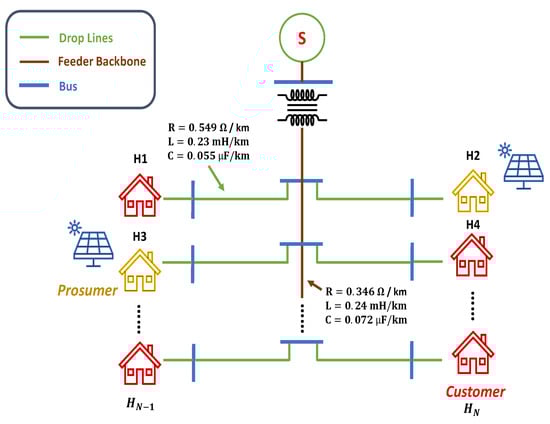
Figure 8.
Simulation test case with a set of 10 customers and 5 prosumers located at different nodes in a radial network based on [34].
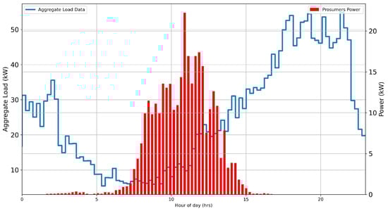
Figure 9.
P2P input data for the suggested trading platform. The data is shown as the double axis graph, where the aggregated PV power of the prosumers is shown in the form of the bar graph with respect to the power axis.
4.1. Trading Results for Interval I
Figure 10 shows the trading results of the different trading strategies for Interval I. Prosumers were able to sell the majority of their PV energy to the P2P customers because of their lower generation and the high demand of the customers (see Figure 10b). Contrarily, due to the relatively lower PV generation of the prosumers, the customers were only able to trade a small amount of their demand from the P2P market (Figure 10a). Figure 10c shows the Interval I welfare metrics using different trading strategies. Because the prosumers sold the majority of their PV energy via the P2P trading platform, their welfare was relatively higher compared to the customers’ welfare, as is evident in Figure 10c. The low welfare of the customers was due to their limited participation in the market because of the relatively lower PV generation of the prosumers. Figure 11 shows the convergence of the Stackelberg game for one of the samples of the market. In this particular sample, the matched orders were (P1-C1, P2-C1, P3-C2, and P4-C3), where P represents the prosumer number, and C represents the customer number. As is evident from Figure 11, the proposed GT approach found the optimal solution while maximizing the utility function of the prosumers’ and the customers’ savings.
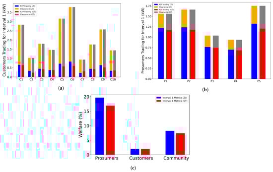
Figure 10.
Comparison of P2P trading results for Interval I for different trading strategies. (a) Customers’ trading pattern for Interval I. (b) Prosumers’ trading pattern for Interval I. (c) Welfare metrics for Interval I.
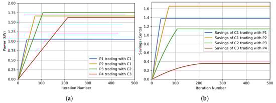
Figure 11.
Convergence of the Stackelberg game for one of the samples of market. (a) Prosumers’ power. (b) Customers’ savings.
Another important aspect for Interval I was that the amount of P2P energy traded using the GT approach was lower compared to the ZI strategy. This resulted in lower welfare for the market participants using GT compared to the rule-based determination. This was due to the fact that the prosumers will have some reluctance () when determining their utility function, which limits their participation in the P2P market. In an ideal case where the prosumers have zero reluctance (), both the ZI and GT methods will yield approximately the same trading results. However, the reluctance parameter is imperative to model the individual preference of the participants under the heavy losses/a network fee, which will be depicted at the later portion of the Section 4. Additionally, to avoid the singularity for the optimization function of the prosumers given in Equation (15), the problem will be solved for . Note that the clearance mechanism (gray portion of the bar graphs) in the results shows the unmatched orders of the P2P market. For customers, the clearance amount is the energy bought from the market operator at the utility real-time price (RTP). Similarly, the prosumers sell any remaining excess PV energy to the operator as a FIT for clearance purposes.
4.2. Trading Results for Interval II
Figure 12 shows the trading pattern for Interval II using different trading methods. For Interval II, the customers traded the majority of their demand from the market due to a relatively higher excess generation of the prosumers compared to the customers’ demand (Figure 12a). The market operator cleared only a small portion of the customers’ demand at the RTP for Interval II. Contrarily, the prosumers traded a small portion of their PV energy with the customers (Figure 12b), but the majority of the PV energy of the prosumers was cleared by the market operator as an FIT. This led to a lower welfare of the prosumers for Interval II when compared to the customers, as is evident from Figure 12c. The same trend was observed for the GT approach, i.e., due to a small value of the , the welfare of the market participants was lower as compared to the ZI strategy.
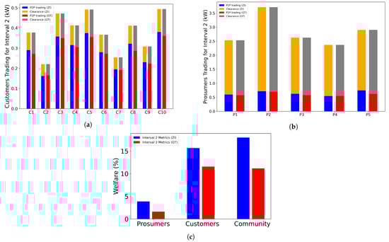
Figure 12.
Comparison of P2P trading results for Interval II (excess PV generation of prosumers was higher compared to the demand of the customers) for different trading strategies. (a) Customers’ trading pattern for Interval I. (b) Prosumers’ trading pattern for Interval I. (c) Welfare metrics for Interval I.
4.3. P2P Traded Energy during Solar Hours
Figure 13 shows the amount of P2P energy traded over the solar hours. From the figure, it is evident that the P2P energy traded between the participants increased for the hours where there was more surplus PV power for the prosumers. For the solar hours where there was less PV energy available, the P2P energy traded also decreased. The amount of traded energy for the ZI strategy was comparatively higher when compared to the GT method, as is explained above.
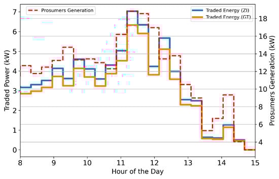
Figure 13.
Comparison of P2P traded energy over the solar hours for each trading strategy. The results are plotted as double axis graph. Dotted plot shows the prosumers’ excess PV power with respect to the second axis.
4.4. Price Comparison and Average Savings of Participants
Figure 14 shows the comparison of the average P2P price versus the RTP and FIT. As is evident from the figure, the participants were offered a price that was competitive to the market values. The customers were offered a price that was lower than the retail tariff, and the prosumers sold their energy at a higher price than the FIT. This resulted in additional saving/earning for the market participants.
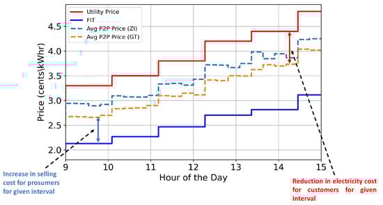
Figure 14.
Comparison of average P2P price with retail and FIT during the solar hours for each trading strategy.
Note that both of the strategies offered an average P2P price that was competitive woth respect to the market values. Table 1 shows the percentage of P2P trading for the different intervals using each trading strategy. The percentage shows the amount of PV energy traded via the P2P market. Table 1 also shows the average monthly savings of the participants. Each customer saved around $3.50, and each prosumer earned an additional $5.80 for the ZI strategy. Similarly, the average savings per participant for the GT approach were $3.25 (per customer) and $5.50 (per prosumer). The monetary advantages for the market participants were established without impairing their comfort factor (shifting of loads). This shows that the presented framework improves the welfare of the P2P community by utilizing the excess PV power of the prosumers in an efficient manner.

Table 1.
Percentage of local trading of P2P energy for the two intervals and average monthly savings.
4.5. Effect of Network Parameters on Welfare of P2P Platform
The welfare of the suggested P2P trading platform depends on the network coefficients such as the loss coefficient, the contribution factor, and the charge rate coefficient. If the distribution/radial network is prone to high losses/a network fee, the welfare of the customers/prosumers can be impaired compared to the ideal market. Under such scenarios, the preference of the participants can play a pivotal role in determining the trading pattern. This research proposes a reluctance-based sensitivity approach for the prosumers to curtail the amount of the traded P2P power for the networks having high distribution losses/a network fee. Note that we only show the effect of network parameters for Interval I. The same conclusions can be made regarding the results for Interval II.
4.5.1. Effect of Contribution Factor
The contribution factor determines the percentage of the network fee that the participants need to pay to the market operator for providing the services. In the suggested network utilization fee model (refer to Equation (20)), the network fee paid by the prosumers depends on the factor (). Contrarily, the customers pay the portion of the total network fee. Hence, by increasing the value of the , the portion of the network fee that the customers need to pay for each energy transaction increases. Contrarily, the network utilization fee decreases by increasing the value of the for the prosumers. Therefore, the prosumers’ welfare is directly proportional to the value of . On the other hand, the customers’ welfare decreases with the increase in the due to the fact that it increases the amount of the utilization fee that customers need to pay for the market services. Figure 15 shows the effect of the contribution factor for the suggested platform. At the intersection point of Figure 15, the found the best compromise between the welfare of both the customers and prosumers. Note that, for the both ZI and GT strategies, the general trend remained same, with the only difference being the lower welfare for the GT method, as is explained above in the Section 4.
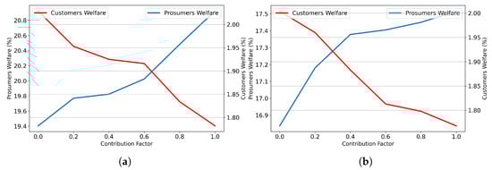
Figure 15.
Effect of the contribution factor on the welfare of the participants for Interval I. (a) ZI strategy. (b) GT approach.
4.5.2. Sensitivity towards Loss Coefficient
Figure 16 shows the effect of the loss coefficient on the prosumers’ welfare for Interval I. It is evident from Figure 16a that if the value of the loss coefficient () was increased to a high value, the welfare of the prosumers became negative. This was due to the fact that, for very high values of , the majority of the PV power of the prosumers was utilized in meeting the losses of the system. A small portion of the P2P power traded by the prosumers was utilized by the customers, which resulted in a negative revenue compared to the traditional market. In the ZI strategy, because the prosumers do not have any preference when determining the amount of traded energy for the matched orders, the P2P energy will remain the same for each value of the loss coefficient. Since at constant value of traded energy , increasing increases the trading losses . Contrarily, for the GT approach, the prosumers can use their reluctance parameter to limit their participation in the P2P market by decreasing the under heavy distribution losses.
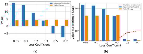
Figure 16.
Prosumers’ welfare for different values of loss coefficient. (a) ZI strategy. (b) GT approach.
Figure 16b shows the trading pattern of the prosumers for different values of the loss coefficient using the GT approach. For high values of the loss coefficient, the prosumers increased their reluctance parameter . This resulted in the limited amount of PV energy traded with the customers that could avoid the negative welfare for the prosumers. Under such circumstances, the prosumers preferred to sell their surplus PV energy to the operator as an FIT. This is one of the main advantages of the suggested GT approach, where the prosumers can adjust their trading pattern based on the network parameters using the parameter .
4.5.3. Sensitivity towards Charge Rate Coefficient
Figure 17 shows the effect of the charge rate coefficient on the welfare of the prosumers for Interval I. The same trend can be observed as with the loss coefficient, where the prosumers’ welfare decreased to a negative value for the ZI strategy. This is because the network utilization fee is directly proportional to the charge rate coefficient . Increasing to a high value results in the prosumers paying more to the market operator as compared to what they will earn from the market for P2P transactions. This results in a negative revenue for the prosumers participating in the P2P market at high values of . For the GT approach, the prosumers increase the value of to decrease the amount of traded energy with the customers. Note that for high values of the charge rate coefficient, the welfare also remains negative for the GT approach. This is because at such values of , the prosumers will have to pay more to the market operator when compared to the revenue they will earn from the P2P market for any amount of energy traded. However, the GT approach manages to limit the welfare of the prosumers to a very small negative value, which is more competitive compared to the ZI results. Because the suggested P2P platform depends on the day-ahead market and intermittent nature of the PV resources, the performance of the presented trading strategies can be improved by introducing the intraday market to model the uncertainty of the PV source. However, this aspect of the suggested P2P platform has been left for future research [35].
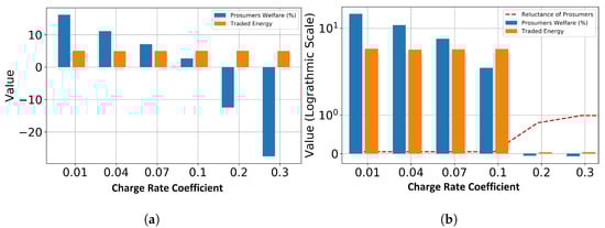
Figure 17.
Prosumers’ welfare for different values of charge rate coefficient. (a) ZI strategy. (b) GT approach.
5. Conclusions
The efficient utilization of the excess PV energy of prosumers can enhance the social welfare of the P2P community. P2P trading platforms using a specific trading mechanism ensures that the surplus PV energy can be shared in a cost-effective manner. This research proposed the comparative analysis of two trading strategies, i.e., the ZI method and GT approach, for a constrained P2P trading platform. The results were simulated over different intervals to show the effectiveness of the proposed trading methods. Additionally, the trading losses and network utilization fee were suggested for incorporating the network constraints. The results show that both of the trading methods give additional monetary advantages for the market participants, while they increased the average welfare by 17%.
A reluctance-based sensitivity approach was also suggested to model the individual preferences of the prosumers under heavy distribution losses/network fees. The GT approach is more beneficial for the networks where there are high losses/a utilization fee as compared to the ZI method, wherein it improved the welfare of the market participants by about 75%. The future research involves adding battery energy storage and an aggregator demand response optimization framework to further enhance the monetary benefits of the market participants for the suggested P2P network.
Author Contributions
Conceptualization, S.L. and T.M.H.; methodology, S.L. and T.M.H.; validation, S.L., T.H., R.F. and F.A.K.; formal analysis, S.L., T.H., F.A.K. and B.C.; writing—original draft preparation, S.L., T.H. and F.A.K.; writing—review and editing, B.C., R.F. and T.M.H.; supervision, T.M.H. and R.F. All authors have read and agreed to the published version of the manuscript.
Funding
This research received no external funding.
Institutional Review Board Statement
Not applicable.
Informed Consent Statement
Not applicable.
Data Availability Statement
The data presented in this study are available on reasonable request from the corresponding author.
Acknowledgments
Sheroze Liaquat thanks the Higher Education Commission (HEC) of Pakistan and the Center of Power System Studies (CPSS) at SDSU for funding this research.
Conflicts of Interest
The authors declare no conflict of interest.
Abbreviations
The following abbreviations and symbols are used in this manuscript:
| P2P | Peer-To-Peer |
| ZI | Zero Intelligent |
| GT | Game Theory |
| FIT | Feed-In Tariff |
| RTP | Real Time Price |
| EM | Equilibrium Matching |
| List of Symbols | |
| Number of Market Intervals | |
| Poission Process | |
| Expected Value of Device Duration | |
| Expected Value of Device Power | |
| , | Scaling Coefficients for Queuing Model |
| Short Circuit Current | |
| Open Circuit Voltage | |
| Series-Connected Modules | |
| Parallel-Connected Modules | |
| , | STC Parameters |
| , | Maximum and Minimum Voltage Levels |
| i | Index of Customer |
| j | Index of Prosumer |
| P2P Price | |
| Demand of Customer | |
| , | P2P Clearance Quantities |
| P2P Loss | |
| Loss Coefficient | |
| Electrical Distance | |
| Network Fee | |
| Contribution Factor | |
| Charge Rate Coefficient |
Appendix A
Table A1 shows the simulation parameters used for the suggested P2P trading platform.
Table A1.
Simulation parameters used for the suggested P2P platform.
Table A1.
Simulation parameters used for the suggested P2P platform.
| Parameter | Value |
|---|---|
| Queuing Load Model Parameters | |
| PJM system operator data for January 1, 2016 for ComEd load area [36] | |
| 500 W [30] | |
| 5 kW [30] | |
| Solar Parameters | |
| Module characteristics | Five different characteristics taken for prosumers given in [32] |
| Rated system capacity | Randomly initialized in range [3, 6 kW] [28] |
| T | Forecast temperature data presented in [28] |
| G | Forecast irradiance data presented in [28] |
| Market Parameters | |
| 96 | |
| 15 min | |
| N | 1000 |
| Retail tariff | ComEd hourly price [37] |
| FIT | ComEd hourly price [37] |
| 0.05 [28] | |
| 0 [28] | |
| 0.03 [28] | |
| 0.001 | |
References
- Liaquat, S.; Zia, M.F.; Benbouzid, M. Modeling and formulation of optimization problems for optimal scheduling of multi-generation and hybrid energy systems: Review and recommendations. Electronics 2021, 10, 1688. [Google Scholar] [CrossRef]
- Cucchiella, F.; D’adamo, I.; Gastaldi, M. Photovoltaic energy systems with battery storage for residential areas: An economic analysis. J. Clean. Prod. 2016, 131, 460–474. [Google Scholar] [CrossRef]
- Soto, E.A.; Bosman, L.B.; Wollega, E.; Leon-Salas, W.D. Peer-to-peer energy trading: A review of the literature. Appl. Energy 2021, 283, 116268. [Google Scholar] [CrossRef]
- Yao, H.; Xiang, Y.; Hu, S.; Wu, G.; Liu, J. Optimal Prosumers Peer-to-Peer Energy Trading and Scheduling in Distribution Networks. IEEE Trans. Ind. Appl. 2021, 58, 1466–1477. [Google Scholar] [CrossRef]
- Tushar, W.; Saha, T.K.; Yuen, C.; Smith, D.; Poor, H.V. Peer-to-peer trading in electricity networks: An overview. IEEE Trans. Smart Grid 2020, 11, 3185–3200. [Google Scholar] [CrossRef]
- Zhang, C.; Wu, J.; Long, C.; Cheng, M. Review of existing peer-to-peer energy trading projects. Energy Procedia 2017, 105, 2563–2568. [Google Scholar] [CrossRef]
- Morstyn, T.; Teytelboym, A.; McCulloch, M.D. Bilateral contract networks for peer-to-peer energy trading. IEEE Trans. Smart Grid 2018, 10, 2026–2035. [Google Scholar] [CrossRef]
- Cali, U.; Fifield, A. Towards the decentralized revolution in energy systems using blockchain technology. Int. J. Smart Grid Clean Energy 2019, 8, 245–256. [Google Scholar] [CrossRef]
- Zhang, C.; Wu, J.; Zhou, Y.; Cheng, M.; Long, C. Peer-to-Peer energy trading in a Microgrid. Appl. Energy 2018, 220, 1–12. [Google Scholar] [CrossRef]
- Morstyn, T.; McCulloch, M.D. Multiclass energy management for peer-to-peer energy trading driven by prosumer preferences. IEEE Trans. Power Syst. 2018, 34, 4005–4014. [Google Scholar] [CrossRef]
- Li, Z.; Ma, T. Peer-to-peer electricity trading in grid-connected residential communities with household distributed photovoltaic. Appl. Energy 2020, 278, 115670. [Google Scholar] [CrossRef]
- Wang, Z.; Yu, X.; Mu, Y.; Jia, H. A distributed Peer-to-Peer energy transaction method for diversified prosumers in Urban Community Microgrid System. Appl. Energy 2020, 260, 114327. [Google Scholar] [CrossRef]
- Angaphiwatchawal, P.; Phisuthsaingam, P.; Chaitusaney, S. A k-Factor Continuous Double Auction-Based Pricing Mechanism for the P2P Energy Trading in a LV Distribution System. In Proceedings of the 2020 17th International Conference on Electrical Engineering/Electronics, Computer, Telecommunications and Information Technology (ECTI-CON), Phuket, Thailand, 24–27 June 2020; pp. 37–40. [Google Scholar]
- An, J.; Lee, M.; Yeom, S.; Hong, T. Determining the Peer-to-Peer electricity trading price and strategy for energy prosumers and consumers within a microgrid. Appl. Energy 2020, 261, 114335. [Google Scholar] [CrossRef]
- Zhou, Y.; Lund, P.D. Peer-to-peer energy sharing and trading of renewable energy in smart communities—Trading pricing models, decision-making and agent-based collaboration. Renew. Energy 2023, 207, 177–193. [Google Scholar] [CrossRef]
- Doan, H.T.; Cho, J.; Kim, D. Peer-to-peer energy trading in smart grid through blockchain: A double auction-based game theoretic approach. IEEE Access 2021, 9, 49206–49218. [Google Scholar] [CrossRef]
- Dong, J.; Song, C.; Liu, S.; Yin, H.; Zheng, H.; Li, Y. Decentralized peer-to-peer energy trading strategy in energy blockchain environment: A game-theoretic approach. Appl. Energy 2022, 325, 119852. [Google Scholar] [CrossRef]
- Lin, J.; Pipattanasomporn, M.; Rahman, S. Comparative analysis of auction mechanisms and bidding strategies for P2P solar transactive energy markets. Appl. Energy 2019, 255, 113687. [Google Scholar] [CrossRef]
- Malik, S.; Duffy, M.; Thakur, S.; Hayes, B.; Breslin, J. A priority-based approach for peer-to-peer energy trading using cooperative game theory in local energy community. Int. J. Electr. Power Energy Syst. 2022, 137, 107865. [Google Scholar] [CrossRef]
- Gokcek, T.; Sengor, I.; Erdinc, O. A novel multi-hierarchical bidding strategy for peer-to-peer energy trading among communities. IEEE Access 2022, 10, 23798–23807. [Google Scholar] [CrossRef]
- Paudel, A.; Sampath, L.; Yang, J.; Gooi, H.B. Peer-to-peer energy trading in smart grid considering power losses and network fees. IEEE Trans. Smart Grid 2020, 11, 4727–4737. [Google Scholar] [CrossRef]
- Guerrero, J.; Chapman, A.C.; Verbič, G. Decentralized P2P energy trading under network constraints in a low-voltage network. IEEE Trans. Smart Grid 2018, 10, 5163–5173. [Google Scholar] [CrossRef]
- Morstyn, T.; Teytelboym, A.; Hepburn, C.; McCulloch, M.D. Integrating P2P energy trading with probabilistic distribution locational marginal pricing. IEEE Trans. Smart Grid 2019, 11, 3095–3106. [Google Scholar] [CrossRef]
- Amanbek, Y.; Kalakova, A.; Zhakiyeva, S.; Kayisli, K.; Zhakiyev, N.; Friedrich, D. Distribution Locational Marginal Price Based Transactive Energy Management in Distribution Systems with Smart Prosumers—A Multi-Agent Approach. Energies 2022, 15, 2404. [Google Scholar] [CrossRef]
- Leong, C.H.; Gu, C.; Li, F. Auction mechanism for P2P local energy trading considering physical constraints. Energy Procedia 2019, 158, 6613–6618. [Google Scholar] [CrossRef]
- Botelho, D.; de Oliveira, L.; Dias, B.; Soares, T.; Moraes, C. Integrated prosumers—DSO approach applied in peer-to-peer energy and reserve tradings considering network constraints. Appl. Energy 2022, 317, 119125. [Google Scholar] [CrossRef]
- Zhao, J.; Wang, Y.; Song, G.; Li, P.; Wang, C.; Wu, J. Congestion management method of low-voltage active distribution networks based on distribution locational marginal price. IEEE Access 2019, 7, 32240–32255. [Google Scholar] [CrossRef]
- Liaquat, S.; Hussain, T.; Celik, B.; Fourney, R.; Hansen, T.M. Day-ahead continuous double auction-based peer-to-peer energy trading platform incorporating trading losses and network utilisation fee. IET Smart Grid 2023, 6, 312–329. [Google Scholar] [CrossRef]
- Hansen, T.M.; Chong, E.K.P.; Suryanarayanan, S.; Maciejewski, A.A.; Siegel, H.J. A Partially Observable Markov Decision Process Approach to Residential Home Energy Management. IEEE Trans. Smart Grid 2018, 9, 1271–1281. [Google Scholar] [CrossRef]
- dos Reis, F.B.; Tonkoski, R.; Hansen, T.M. Synthetic residential load models for smart city energy management simulations. IET Smart Grid 2020, 3, 342–354. [Google Scholar] [CrossRef]
- Eick, S.G.; Massey, W.A.; Whitt, W. Mt/G/∞ Queues with Sinusoidal Arrival Rates. Manag. Sci. 1993, 39, 241–252. [Google Scholar] [CrossRef]
- Ortiz-Rivera, E.I. Approximation of a photovoltaic module model using fractional and integral polynomials. In Proceedings of the 2012 38th IEEE Photovoltaic Specialists Conference, Austin, TX, USA, 3–8 June 2012; pp. 2927–2931. [Google Scholar]
- Tushar, W.; Chai, B.; Yuen, C.; Huang, S.; Smith, D.B.; Poor, H.V.; Yang, Z. Energy storage sharing in smart grid: A modified auction-based approach. IEEE Trans. Smart Grid 2016, 7, 1462–1475. [Google Scholar] [CrossRef]
- Tonkoski, R.; Lopes, L.A.C.; El-Fouly, T.H.M. Coordinated Active Power Curtailment of Grid Connected PV Inverters for Overvoltage Prevention. IEEE Trans. Sustain. Energy 2011, 2, 139–147. [Google Scholar] [CrossRef]
- Garcia-Guarin, J.; Alvarez, D.; Rivera, S. Uncertainty Costs Optimization of Residential Solar Generators Considering Intraday Markets. Electronics 2021, 10, 2826. [Google Scholar] [CrossRef]
- PJM Data Miner. Available online: https://dataminer2.pjm.com/list (accessed on 21 February 2022).
- ComEd Hourly Price. Available online: https://hourlypricing.comed.com/live-prices/ (accessed on 21 February 2022).
Disclaimer/Publisher’s Note: The statements, opinions and data contained in all publications are solely those of the individual author(s) and contributor(s) and not of MDPI and/or the editor(s). MDPI and/or the editor(s) disclaim responsibility for any injury to people or property resulting from any ideas, methods, instructions or products referred to in the content. |
© 2023 by the authors. Licensee MDPI, Basel, Switzerland. This article is an open access article distributed under the terms and conditions of the Creative Commons Attribution (CC BY) license (https://creativecommons.org/licenses/by/4.0/).