Abstract
The target simulation of airplanes is an important research topic. It is particularly important to find the right balance between high performance and low cost. In order to balance the contradictions between realistic target simulations and controllable costs, the scientific formulation of the performance parameters of target simulation is the key to achieving high performance. This paper proposes an intelligent simulation technology based on RCS imaging simulation through the combination of 60° variation corner reflector and a Luneberg lens reflector. It is designed to simulate several important RCS characteristics of the aircraft. At the same time, the different RCS images are automatically shifted to the corresponding gear position to achieve the purpose of simulation, and the price is low and the performance is good. It can be used for the training of radar target searching.
1. Introduction
At present, the methods for aircraft simulation at home and abroad mainly include target characteristics simulation [1,2,3,4] and motion characteristics simulation [5,6,7,8]. In order to improve the function coverage of target drones, it is necessary to develop the technology for simulating variable radar scattering characteristics. The commonly used RCS enhancement techniques include: dielectric reflectors, corner reflectors and Luneberg lens reflectors. A Luneberg lens reflector can focus electromagnetic waves and reflect them out with a high gain, and significantly increase the RCS in a specific angular range. Furthermore, the beamwidth can be adjusted according to the size and position of the reflector. However, its disadvantage lies in the high requirements for the process. The corner reflector material is a common metal with low technological level requirements. Its interface stiffness is high, the price is low and it can meet the needs of the target. Therefore, corner reflectors or Luneberg lenses are commonly used to simulate the radar scattering characteristics of targets [9,10,11,12,13,14,15,16,17,18,19].
In China and other countries, Luneberg lens reflectors and corner reflectors have also been subjected to a lot of research in other aspects.
The Luneberg lens reflector is also used in the fields of military target aircraft, calibration reflectors, target indicators or simulators, navigation beacons, targets, buoys, etc. For example, the Luneberg lens reflector with a diameter of 0.3 m can simulate a radar target aircraft of a heavy bomber. In civilian use, fishermen’s boats are usually equipped with Luneberg lens reflectors, so that our radar can detect them and carry out search and rescue in rainstorm weather. At the same time, Luneberg lens reflectors can also be used as an antenna; the most widely used is in satellite communication systems, because compared with parabolic satellites on the ground, Luneberg lens reflectors can achieve beam control and a large angle range of 120°. They can also focus the incident electromagnetic wave [20]. In addition, many companies have also conducted research on the production of Luneberg lens reflectors, and launched many practical commercial products, such as France’s high-speed train satellite antenna, Australia’s Luneberg lens reflector array, Japan’s lens antenna in the new wind measurement radar, and Egypt’s Dr. Farag made a multi-feed source helmet lens antenna [21].
In 2005, Zhang Bo et al. [22], aiming at the background characteristics of a bridge’s water surface, started with changing the RCS value of the bridge’s exposure characteristics, and realized the simulation of the bridge’s false target by means of a corner reflector array at a suitable position and coating with absorbing materials. In 2009, Royason et al. [23] proposed a decoy array simulation RCS model and calculation method, and calculated the RCS of the angular reflector array of a ship at sea. This method solved the problem of the model complexity and low calculation efficiency relate to the large electrical size. In the same year, Zhang Ning et al. [24] established a mathematical model for the approximate calculation of pier RCS, filtering the target area based on structural analysis and using sliding windows for assignment, which effectively reduced the number of local windows involved in the calculation, and set the corner reflector array of an anti-radar fake pier according to the model. Yan et al. modified the diagonal reflector structure and installed a metamaterial absorber to maintain the same RCS distribution characteristics at 8 GHz and 12 GHz, which could effectively cope with radar detection [25]. Hao et al. realized the variable RCS of the corner reflector by rotating the side of the corner reflector, which could simulate objects considerably larger than itself, but it was not possible to simulate complex targets [26]. Zhang et al. modified and enhanced the target RCS by adding the Luneberg lens under the nose of a target drone [27].
This paper proposes an intelligent simulation technology based on RCS imaging simulation. It can simulate the typical RCS characteristics of aircraft by mutating the structure of the 60° corner reflector and combining it with the Luneberg reflector. At the same time, Doppler frequency simulators with many speed gears from 0 to 200 km/h are designed to simulate the speed of an airplane. In this paper, an aircraft simulator with a high accuracy of RCS distribution characteristics, wide range of Doppler effect simulation, high performance index and low cost is studied, which has wide research significance and application value.
2. Target Drone Simulation Principle
2.1. Variable Principle of Corner Reflector
The RCS of the target is used to represent the intensity of the signal reflected back to the radar receiver after the radar transmitter emits an electromagnetic wave towards the surface of the target. It is a physical quantity indicating the scattering ability of the target scatterer to the radar transmitted wave. It is defined as times the ratio of the power scattered by the target in the receiving direction and the plane wave power density incident at the target from a given direction in a unit solid angle. It is denoted by , and can be expressed as follows:
where represents the radar–target distance, and , and represent the energy flow density, electric field strength, and magnetic field strength of the target echo signal received by the radar, respectively. The energy flow density, electric field strength, and magnetic field strength of the radar transmitting signals to the target are denoted by , and , respectively.
The RCS value is scalar, measured in square meters. Its logarithmic representation is commonly used in practical applications, i.e., for the number of decibels per square meter (also known as decibel square meter, denoted as dBsm), and the expression is as follows:
The variable RCS properties of corner reflectors can be further analyzed by considering the angle, frequency, polarization mode, and the number of reflections of the incident wave. Usually, electromagnetic calculation methods such as Geometrical Optics (GO), Area Projection (AP), and Physical Optics (PO) are used for analysis. The traditional GO algorithm can effectively calculate the RCS value of a trihedral corner reflector. However, as it is a high-frequency approximation method, it considers the electromagnetic wave as a beam with a wavelength of 0, which makes it impossible to analyze the polarization mode of the incident wave. The PO method cannot be further extended and applied to irregular corner reflectors with more complex structures due to its inability to calculate the irradiation area. Therefore, this article uses the PO-AP algorithm to analyze the omnidirectional RCS of the diagonal reflector model.
Assuming that the metal flat plate forming the corner reflector is an ideal conductor, the reflecting object will induce twice the current corresponding to the incident tangent magnetic field on its surface, where is the normal vector of the reflector surface. The reflected magnetic field at the observation point, whose distance from the origin is , can be determined by the PO method as follows:
where is the incident magnetic field that reaches the surface of the reflecting object, while and are the unit and distance vectors from the incident point to the origin, respectively. Equation (4) integrates the area where electromagnetic waves irradiate the reflector.
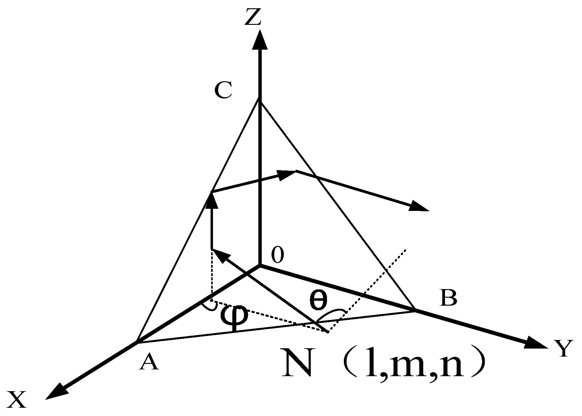
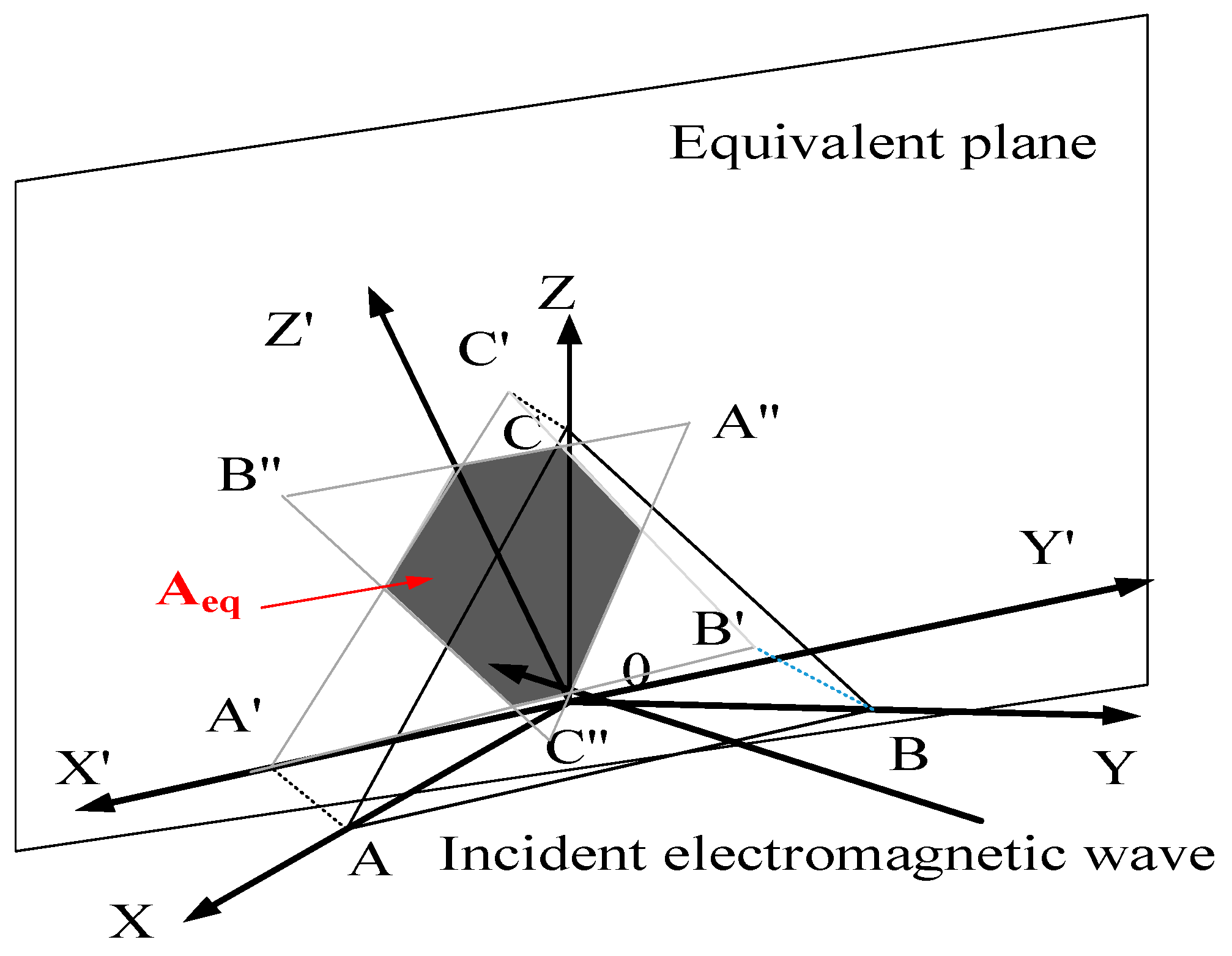
The incident wave may be reflected zero to three times inside the corner reflector, and only three reflected echoes will return to the radar receiver along the path of the original incident direction. Thus, three reflections within a large angular range form the main contributing source of the corner reflector RCS, while up to two reflections can be ignored when calculating the monostatic RCS. The ability of the incident wave to be reflected three times depends on the mutual determination of the incident point P and the incident direction. When a plane wave is at an infinite position, all three reflected echoes have equal phases. Therefore, when the RCS value is calculated using the PO method, an angular reflector can be equivalent to a plane of some dimension through the vertex and orthogonal to the direction of incident, which is the “equivalent aperture”. The incident direction of the electromagnetic wave . Figure 1 shows the schematic diagram of the triple-bounce of the corner reflector.
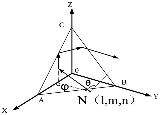
Figure 1.
Schematic diagram of the triple-bounce of the corner reflector.
The expression of the incident magnetic field is
where is the unit vector representing the magnetic field direction, while and are the unit and distance vectors from the incident point to the origin, is the amplitude, and d is the distance vector from the incident point to the origin. Let , and be the unit vectors along the X, Y and Z axes, respectively. Subsequently, the unit vectors and can be obtained as follows:
where is the polarization angle of the electric field at the incident point, e.g., vertical polarization means that this angle is 0°.
Therefore, the three reflections of incident electromagnetic waves on the corner reflector can be obtained from (5) as
where and are the normal vectors of the reflection surfaces and , respectively.
The total reflected magnetic field is composed of a combination of the re-radiation of the aforementioned incident magnetic field. There are six combinations, namely, , , , , and .
After putting (6) into (4), reflected three times on the corner reflector can be obtained as follows:
By substituting (7) into (1), the RCS value of the incident point can be obtained as follows:
In order to simplify the RCS calculation of complex structures, the RCS of the variable corner reflector can be calculated only by obtaining the shape of the “equivalent aperture”. Subsequently, the shape can be integrated to obtain its area , which is determined by regional projection.
Firstly, the reflector structure has multiple scattering centers. Therefore, the RCS of target scattering center is required. The transfer function of multiple scattering centers is defined as:
where is the scattered electric field, is the scattered electric field, is the frequency, is the world, and is the wave number, .
The above transfer function references the spherical wave transfer factor, and according to this definition, the RCS of the target scattering center is:
After the equivalent aperture is projected onto the equivalent plane, it can be regarded as an irregular plane, and for specular reflection on a flat plate, the transfer function is:
Therefore, the RCS value of the equivalent aperture is:
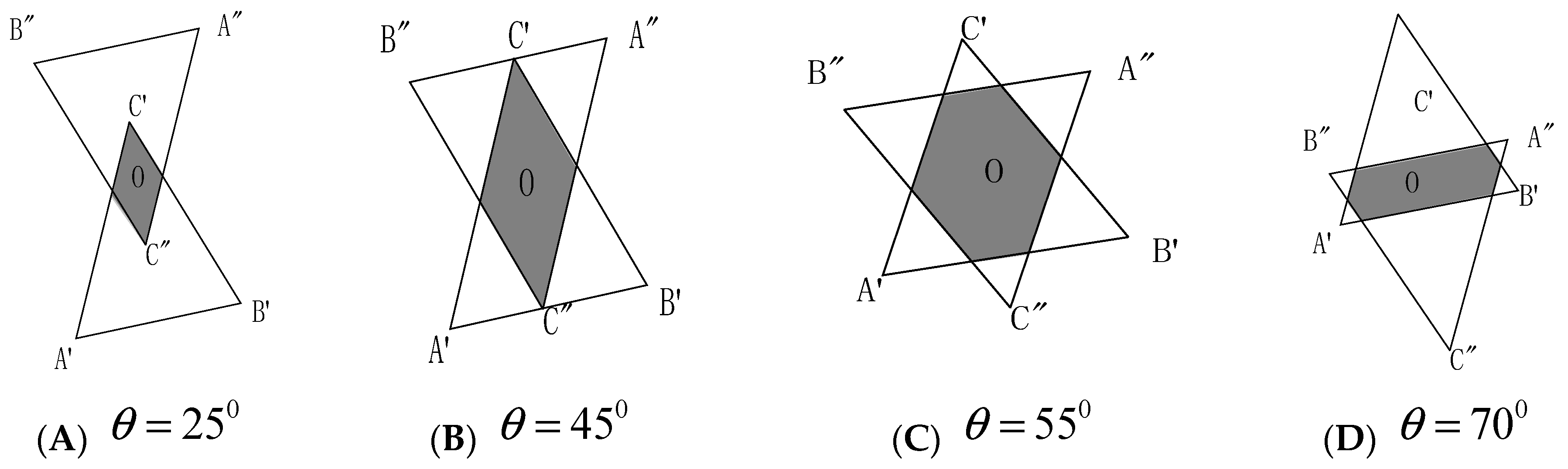
A spatial coordinate system is established where the virtual and real apertures are located. The real and virtual aperture triangles are denoted by and , respectively. The origin of the spatial coordinate system where the real aperture is located is still at point O. The , and axes extend in the , and directions, respectively. The area covered by triple reflection in a corner reflector is usually a parallelogram or hexagonal, as shown in Figure 2.
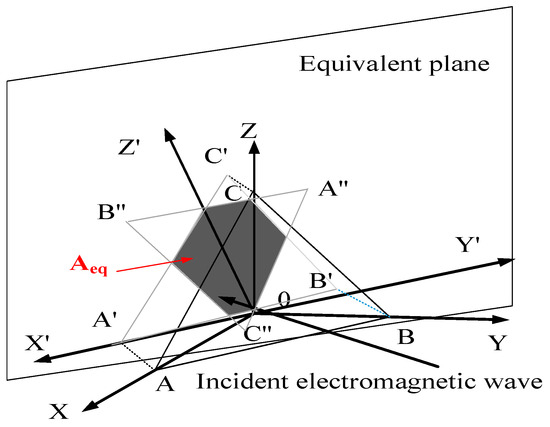
Figure 2.
Schematic diagram of the equivalent plane of the corner reflector.
In order to simplify the RCS calculation of complex structures, the RCS of the variable corner reflector can be calculated only by obtaining the shape of the “equivalent aperture”. Subsequently, the shape can be integrated to obtain its area , which is determined by regional projection. In this way, the RCS can be used to estimate the angular reflector when the plane wave containing the wavelength is vertically incident on the plate:
Figure 3 shows the variation of with when .

Figure 3.
Variation of trihedral corner reflector area with .
2.2. Luneberg Lens Reflector
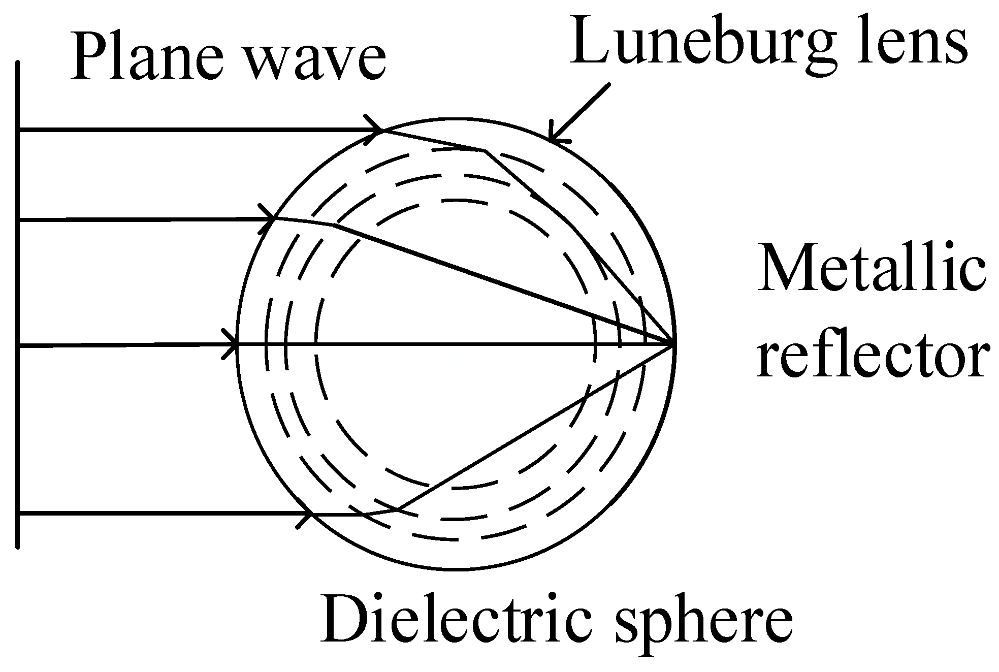
The Luneberg lens reflector is a passive reflector made by coating a layer of metal reflector on the surface of a Luneberg ball according to the principle of light reflection and refraction in a passive medium [15,16]. The ideal Luneberg lens reflector is a mirror-symmetric spherical structure that has a continuous gradient of permittivity along the radius of the ball. The permittivity of the Luneberg ball changes from 2 in the center to 1 on its surface. The relative permittivity of the outermost medium of the reflector is the same as or close to that of air. The reflector has a refractive index of 1.414 at the center of the sphere and gradually decreases to 1 at its outermost layer.
The gradient nature of the medium of the Luneberg lens ball makes it an excellent focusing system, as shown in Figure 4.

Figure 4.
Schematic diagram of Luneberg lens.
The Luneberg lens is a spherical lens whose refraction coefficient is a function of the distance from the center of the sphere to its surface, as expressed below:
where represents the distance between the center of the sphere and the outer surface of the medium sphere, and represents the radius of the Luneberg lens.
The dielectric constant of each dielectric spherical layer is
Using (11), the relative dielectric constant of the corresponding dielectric layer of Luneberg lens can be calculated.
2.3. Doppler Signal Generation
Assuming that the target is an ideal target, i.e., the target size is considerably smaller than the radar resolution unit, the transmitted signal can be expressed as:
where represents the amplitude of the transmitted signal, represents the angular frequency of the transmitted wave signal, and represents the initial phase. Subsequently, the echo signal received from the moving target can be expressed as:
where represents the attenuation coefficient and represents the time delay of the radar signal from the transmission to reception.
If the target is stationary, the time delay represented by has a constant value of 2R/c. If the target moves with a certain speed, the distance R changes with the change of time t, namely:
The phase difference can be expressed as:
The derivative of the phase difference can be obtained as:
At this point, the speed of the moving target is:
Similarly, if the target is stationary, in Equation (2) has a constant value. Consequently, is a fixed value. However, the environment around the target is not static when the target is measured. As an example, if the wind blows the trees, the leaves will produce vibration, and flowing rivers will produce a large amount of clutter interference, which will affect the Doppler frequency deviation.
In this paper, the oscillation circuit is used to simulate the Doppler frequency corresponding to the velocity. Here, Figure 5a shows the schematic diagram of a capacitor-based three-point LC oscillation circuit. The oscillation frequency is , where . Although the oscillating waveform produced by this circuit structure is utility, it is difficult to adjust the frequency of the generated oscillating waveform. Therefore, this circuit is only suitable for a high fixed frequency. The most widely used sinusoidal oscillators are LC and RC oscillator circuit structures.
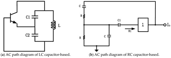
Figure 5.
Two types of oscillating circuits.
In the sinusoidal oscillation circuit shown in Figure 5b, the oscillation frequency is . The oscillation waveform output by this circuit structure has a stable frequency and no distortions. The amplitude of the output waveform can be stabilized by adding negative feedback, which makes it suitable for applications requiring an adjustable frequency.
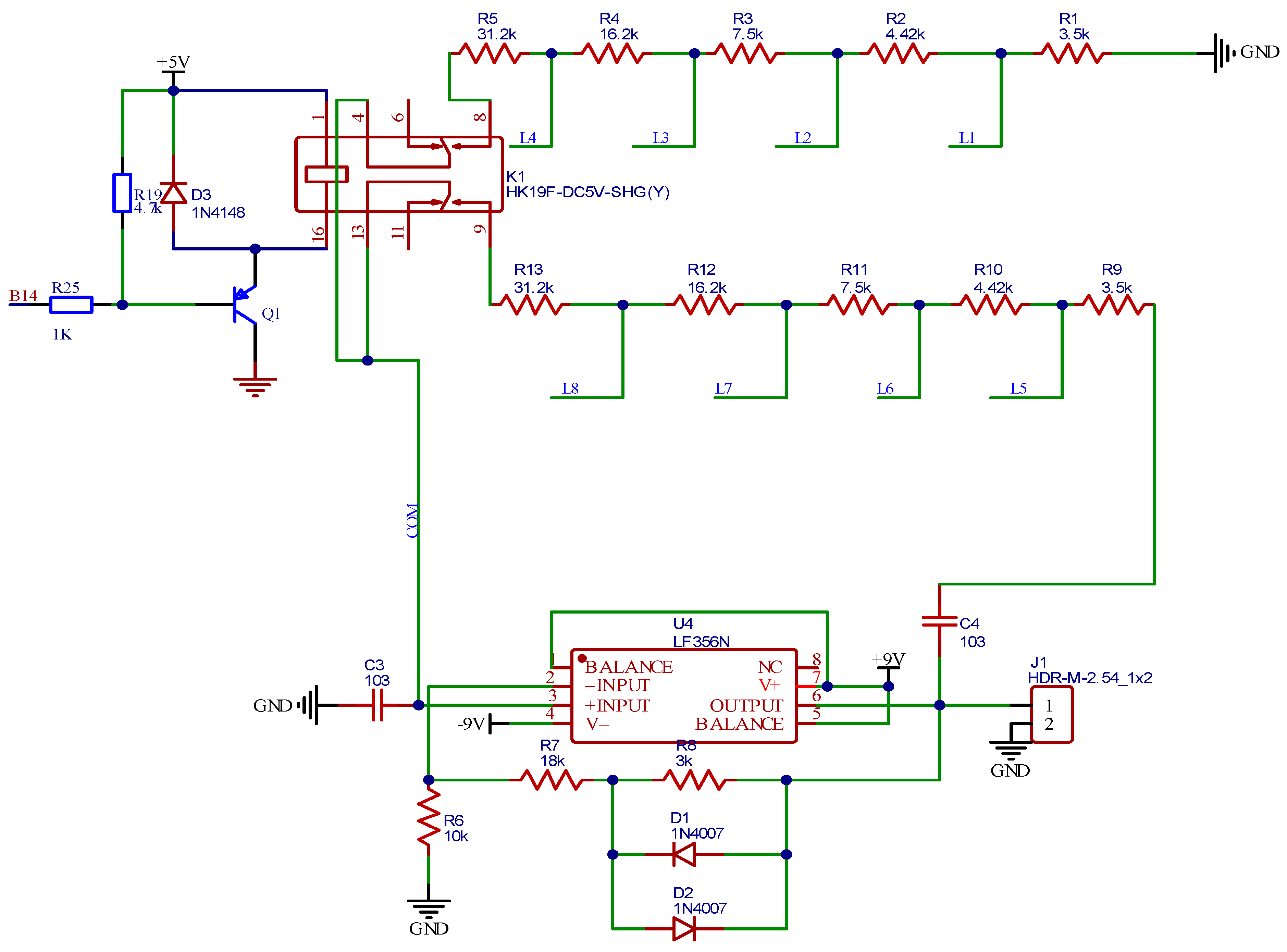
To evaluate the performance of the Doppler frequency simulator, a 10 GHz frequency test system is designed for experimental verification, as shown in Figure 6. A speed of 0–200 km/h is simulated, divided into six levels: 0 km/h, 12.5 km/h, 25 km/h, 50 km/h, 100 km/h and 200 km/h. According to Equation (6), the corresponding analog frequencies can be calculated at 0, 230 Hz, 460 Hz, 925 Hz, 1.96 kHz, and 4 kHz. The voltage of the 4 kHz oscillation circuit is ±9 V, R1 and R2 are equal to 62.82 kΩ, C3 and C4 are equal to 0.01 μF, R7 is 18 kΩ, R4 is 10 kΩ and R8 is equal to 3 kΩ. The two diodes constitute a nonlinear network, which can render the amplifier of the circuit stable over 3 repetitions [28]. This prevents the distortion of the output waveform and ensures its stability. The opamp uses LF356n. Since it is a single-stage common emitter amplifier circuit, the output voltages of the transistor and are 180° in phase. When the output voltage passes through the RC network, it becomes the feedback voltage, and then sends this to the input end. L1-L8 are eight LED lights, and the communication status of the communication interface is determined by the blinking of the LED lights.
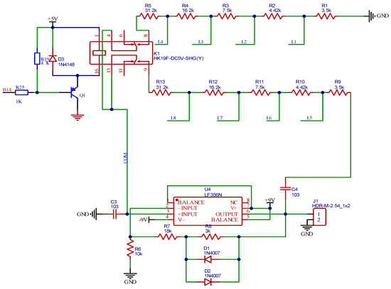
Figure 6.
Design of Doppler frequency simulator with adjustable speed gear.
2.4. Fidelity Evaluation Model
Fidelity is a measure of the closeness of the simulation to the real world and is the key to simulation verification.
The factors that affect the energy domain’s fidelity are mainly caused by the power intensity. For the target simulation, the power error is mainly reflected in the RCS (dBsm), or the energy proportion within the peak width. To evaluate the RCS peak index model, the error range between the RCS value (a) of the simulated aircraft and the RCS value (b) of the reference object need to be determined. Assuming an allowable error range of ±3 dB, when the difference between (a) and (b) is within this range, the fidelity is considered to be up to standard. The following expression can be used to provide a fidelity score within the error range, while mapping the normal distribution model’s score to the [0, 100] range:
where is the weight coefficient of the corresponding part, represents the difference between the RCS values of the simulated target and the reference object, and is the standard deviation of the error.
The fidelity score can be calculated to determine whether the simulation is realistic. The fidelity evaluation is shown in Table 1.

Table 1.
Fidelity evaluation index.
3. Target Simulation Modeling and Analysis
An aircraft’s RCS is mainly composed of three parts: sharp angle RCS distribution characteristics, stationary spatial distribution region, and some fluctuations caused by multiple scattering. It becomes very complicated to directly simulate the entire horizontal 360° space region of an aircraft. Therefore, the typical characteristics of the aircraft’s horizontal position, including nose, wing and tail, are described in the following. The design of these three parts can help to effectively realize the target drone simulation [29].
(1) Nose −30°~30° scheme design.
The nose simulation assembly is mainly composed of a 60° variable corner reflector and two Luneberg lens reflectors, wherein the vertical side length of the corner reflector is 600 mm and the diameter of the Luneberg lens is 83 mm. The scanning angle range is as follows: azimuth dimension −90°~90°, pitch dimension 0°, angular scanning interval 1°. Figure 7 and Figure 8 show the composite simulation model and the RCS distribution characteristics, respectively.

Figure 7.
Combination simulation model.
Figure 8.
Radar cross section comparison results from −30° to 30°.
As Figure 8 shows, the RCS distribution characteristics of the assembly have an error of about 0.3 dBsm at the maximum RCS of 0 degrees compared with the distribution characteristics of the head, which meets the requirements. Meanwhile, the sharp angle range of −3°~3° is also consistent, which fulfills the design requirements.
(2) Wing −30°~30° scheme design.
The wing assembly is mainly composed of a tetrahedral variant assembly with a side length of 780 mm and two metal balls with a diameter of 192 mm. These balls are mainly used to reduce the edge diffraction of the corner reflector. The scanning angle range is as follows: azimuth dimension −90°~90°, pitch dimension 0°, angle scanning interval 1°. Figure 9 and Figure 10 show the composite simulation model and the RCS distribution characteristics, respectively.

Figure 9.
Combination simulation model.
Figure 10.
Radar cross section comparison results from −30° to 30°.
As Figure 10 shows, the RCS distribution characteristics of the assembly have an error of about 0.02 dBsm at the maximum RCS of 0° compared with the distribution characteristics of the head, which meets the requirements. Meanwhile, the sharp angle range of −3°~3° is also consistent.
(3) Tail −30°~30° scheme design.
The tail simulation assembly consists of a 60° variable corner reflector, a Lombo ball reflector and two metal balls. The vertical side length of the corner reflector is 540 mm, and the diameter of the Lombo ball is 83 mm. The scanning angle range is as follows: azimuth dimension −90°~90°, pitch dimension 0°, angle scanning interval 1°. Figure 11 and Figure 12 show the composite simulation model and the RCS distribution characteristics, respectively.
Figure 11.
Combination simulation model.
Figure 12.
Radar cross section comparison results from −30° to 30°.
As Figure 12 shows, the RCS distribution characteristics of the assembly have an error of about 0.05 dBsm at the maximum RCS of 0° compared with the distribution characteristics of the head, which fulfills the requirements. Meanwhile, the sharp angle range of −3°~3° is also consistent.
4. Analysis of Experimental Results
The performance of the composite object is evaluated by designing a 10 GHz frequency test system for experimental verification. Figure 13 shows the system.

Figure 13.
Test system for the processed physical object.
The computer uses the serial debugging assistant software to send the corresponding instruction statements for controlling the start of RF transceiver components and the setting of parameters. The horn antenna is used as the transceiver antenna of the test system. The vector network analyzer is used to set the transmitting continuous wave point frequency. Figure 14 shows the actual product processed according to the simulation model.
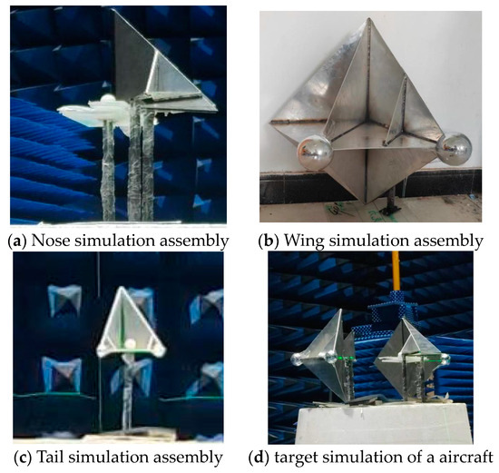
Figure 14.
Target simulation of each part.
Figure 15 shows the test results. It can be observed that when the simulated target drone is placed horizontally at the frequency of 10 GHz, the peak RCS values appear around −180°, −152°, −90°, −39°, −9°, 0°, 9°, 39°, 90° and 152°. The RCS values at −180°, −152°, −90°, −39° and −9° are 21.26 dBsm, 12.37 dBsm, 38.17 dBsm, 17.14 dBsm and 13.09 dBsm, respectively. The RCS values at 0°, 9°, 39°, 90° and 152° are 25.49 dBsm, 12.66 dBsm, 17.14 dBsm, 38.97 dBsm and 12.37 dBsm, respectively. The RCS value at 0° is 1.39 dBsm compared with the corresponding actual value of an aircraft, and the RCS values at other peaks also decreases within 3 dBsm of the aircraft. The test results show that the assessment index of less than 3 dBsm test error is satisfied. Equation (18) shows that the fidelity score is 93.1 points, which indicates a very realistic level and high performance of the simulation, according to Table 1. When the vector network analyzer is measuring, there will be a fluctuation of ±1 dB, which is a systematic error. Therefore, at the position of the symmetric angle, the RCS value will include a certain test error, but as long as it does not exceed 1 dB, the test result can be proven to be correct.
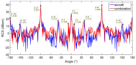
Figure 15.
Radar cross section distribution characteristics of the target simulation.
Deep learning algorithms fall into the following four main categories: convolutional neural networks, recurrent neural networks, generative adversarial networks, and reinforcement learning networks. The convolutional neural network includes a convolutional layer, a pooling layer and a fully connected layer, which is used to learn the features in the image and perform classification and detection. Figure 16 shows the classification of deep learning algorithms.
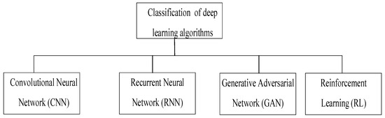
Figure 16.
Classification of deep learning algorithms.
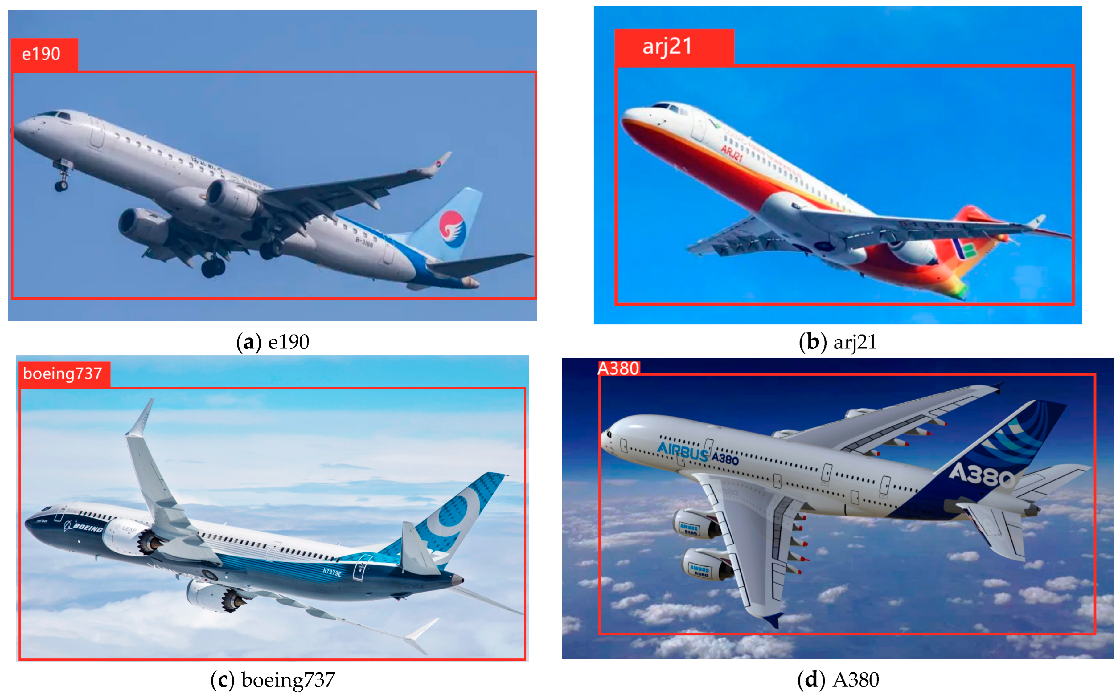
Therefore, the simulated targets are added into a data set and classified by fuzzy clustering or deep learning algorithms. Figure 17 shows the schematic diagram of intelligent shifting for target recognition. The data are collected through the data acquisition module of the single chip microcomputer, and then transmitted to the computer by Wi-Fi. When the identification result is one of the classification results in 1–4, the computer transmits instructions to the relay of the single side machine, and the relay closes the corresponding gear and outputs the corresponding Doppler frequency characteristics. Examples of simulation targets include four types of aircraft, marked as 1, 2, 3 and 4, respectively. Figure 18 shows the classification results.
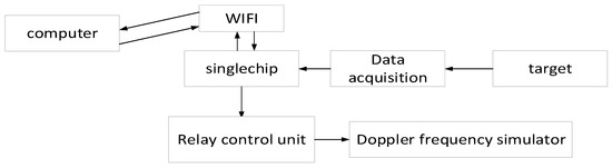
Figure 17.
The schematic diagram of intelligent shifting for target recognition.
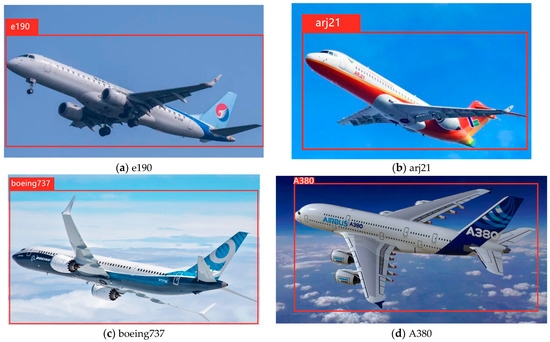
Figure 18.
Identification result of four aircrafts.
The vector network analyzer sets the transmitting continuous wave point frequency. According to the Nyquist sampling theorem, . The specific parameters are shown in Table 2.
Table 2.
Parameter settings.
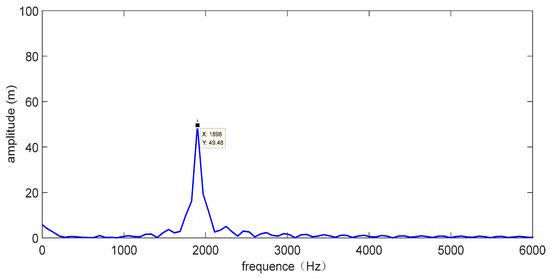
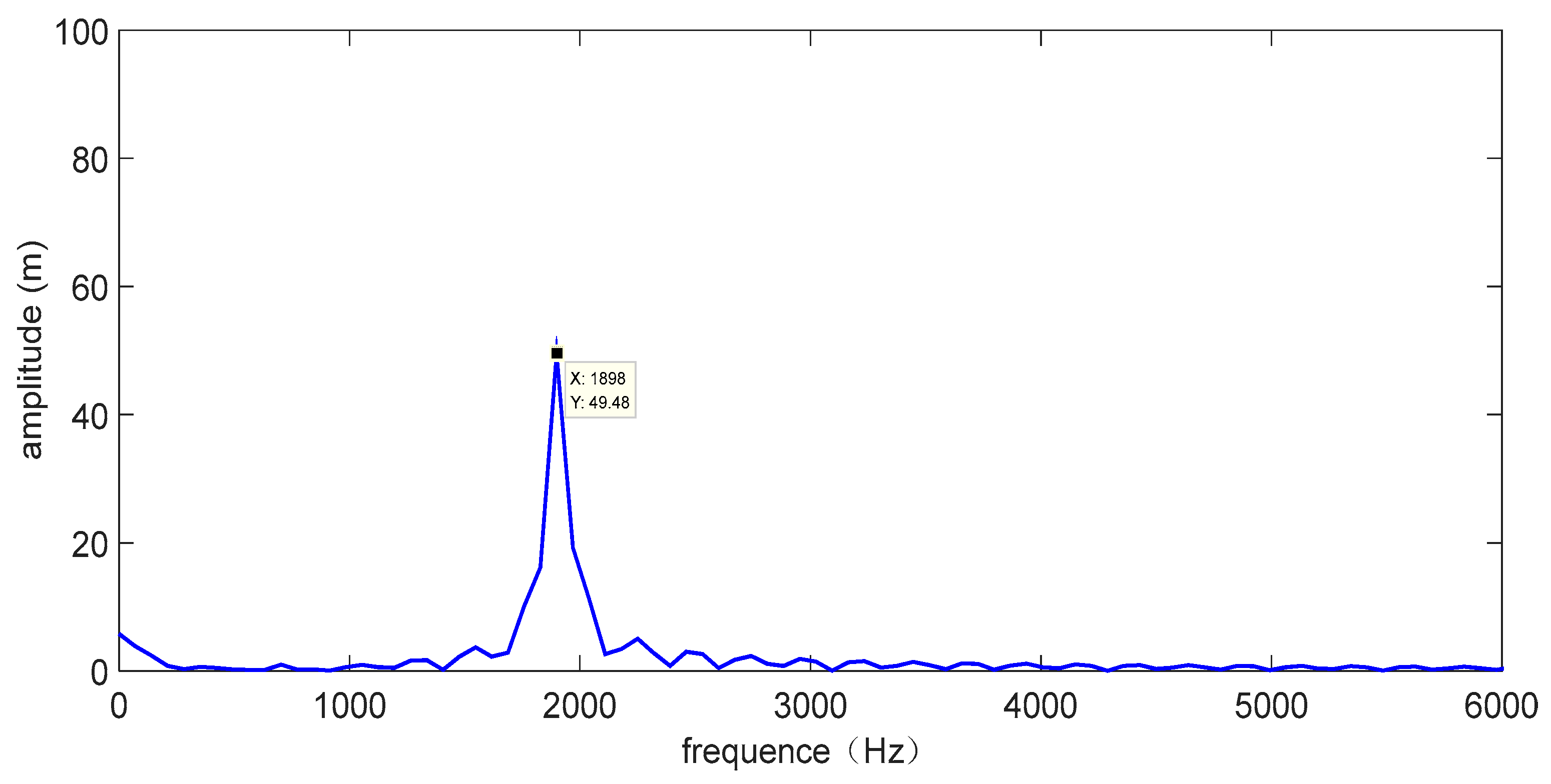
Figure 19.
Speed level: 100 km/h (simulator oscillation frequency: 1.96 kHz).

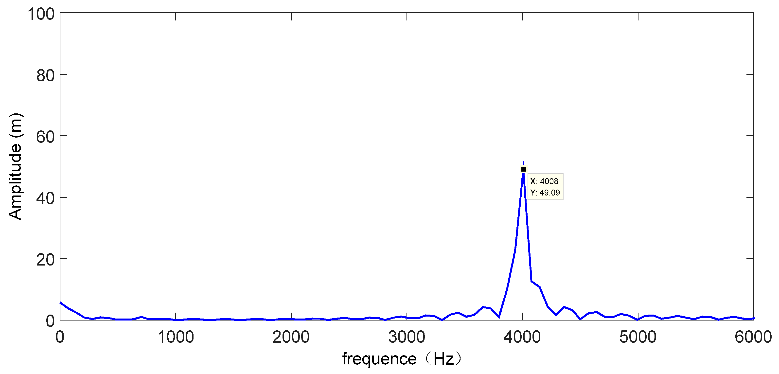
Figure 20.
Speed level: 200 km/h (simulator oscillation frequency: 4 kHz).
Figure 19 and Figure 20 show that the simulated Doppler frequency components appear on the processed spectrum, which verifies the effectiveness and accuracy of the Doppler frequency simulator proposed in this paper.
For the simulation of different speed characteristics, the error between the frequency of the Doppler frequency simulator and the Doppler frequency detected by radar echo is shown in Table 3.
Table 3.
Error analysis of Doppler frequency shift simulator.
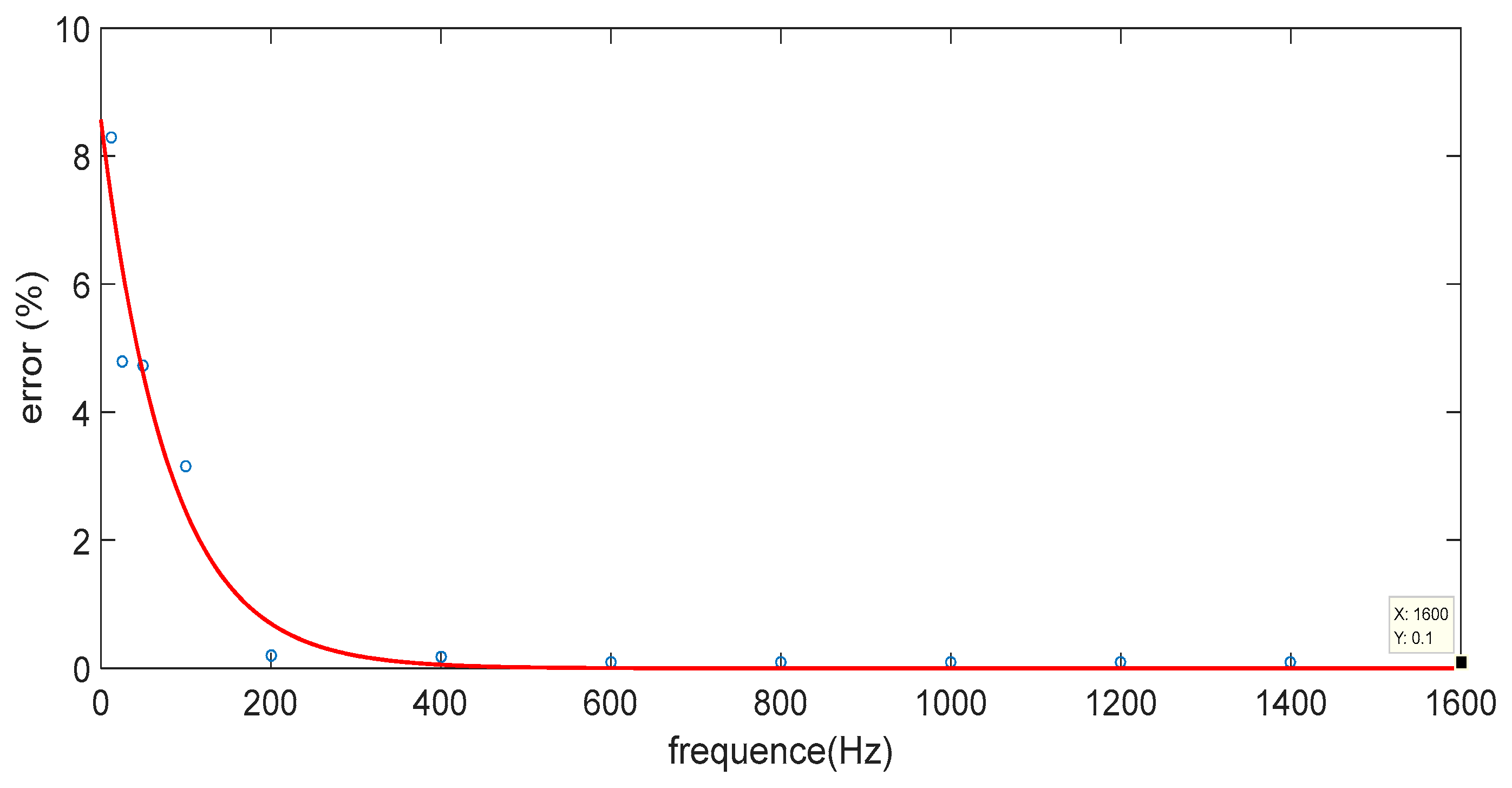
Then, according to the frequency error corresponding to the speed gear in Table 2, the corresponding error variation trend chart is obtained, as shown in Figure 21.
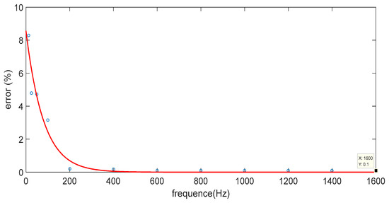
Figure 21.
Error analysis trend chart.
According to Figure 21, the faster the speed, the larger the Doppler frequency, and the smaller the corresponding Doppler frequency error. When the speed gear reaches the maximum speed of the aircraft (about 1600 km/h), the Doppler frequency is 3.2 MHz, and the corresponding error is about 0.1%
Aircraft speed simulation needs ≥1.3 Ma. The RCS distribution characteristics of the aircraft simulator designed in this paper have high simulation fidelity, the speed meets the requirements of aircraft simulation, and the flight duration is 2 h. Compared with other aircraft simulators, the flight duration is longer and the cost is only 10,000 RMB. The JC-80 has a short endurance, and the S-400 meets the needs of aircraft simulation, but the cost is higher. The specific performance comparison is shown in Table 4.
Table 4.
Cost effectiveness analysis.
5. Conclusions
Target simulation technology is very important in radar detection. This paper presented a cost-effective target drone design based on RCS characteristic simulations. The main conclusions are as follows:
- The PO-AP method was used to analyze the RCS of the variable corner reflector, which made up for the shortcomings of the traditional PO method that could not calculate a complex model. A simulation target of an aircraft was designed;
- The distribution characteristics of sharp angle RCS, stationary space region distribution characteristics and fluctuations caused by multiple scatterers of an aircraft were simulated by combining the corner reflector, Luneberg lens reflector and metal sphere. The RCS error of the nose was 1.39 dBsm, while the error of other parts was less than 3 dBsm, which satisfied the design index;
- A fidelity evaluation model for complex targets was proposed, and the designed simulation target drone scored up to 93.1 points, indicating a highly realistic level. This provided an objective and reliable fidelity evaluation rule for complex targets and provided a relevant theoretical basis;
- The Doppler frequency simulator designed in this paper can simulate the motion characteristics of an aircraft, with errors of 8.3% and 4.8%, respectively, which can meet the test requirements.
Author Contributions
Conceptualization, X.W.; methodology, J.H.; investigation, S.Y.; formal analysis, H.G.; software, J.H. All authors have read and agreed to the published version of the manuscript.
Funding
This research was funded by Ministry of Education of the People’s Republic of Chinagrant number (20190209400011).
Institutional Review Board Statement
Not applicable.
Informed Consent Statement
Not applicable.
Data Availability Statement
Not applicable.
Conflicts of Interest
The authors declare no conflict of interest.
References
- Tang, Y.; Qian, P.; Zhang, B. Development status and prospect of radar target echo simulation technology. Aerosp. Electron. Countermeas. 2019, 36, 28–34. [Google Scholar]
- Guo, B.; Kong, X.L.; Sun, H.X.; Zhang, Y.; Li, Y.B. Research on Simulation method of helicopter radar Characteristics. Aeronaut. Sci. Technol. 2019, 30, 57–61. [Google Scholar]
- Li, Y.W. Simulation and simulation analysis of ship target radar echoes. Ship Sci. Technol. 2018, 40, 79–81. [Google Scholar]
- Cai, W. Design and Implementation of Target Simulation System for Wideband Radar. Master’s Thesis, Nanjing University of Aeronautics and Astronautics, Nanjing, China, 2015. [Google Scholar]
- Yu, X.C.; Li, J.W.; Fan, W.; Zhang, Z.; Zhao, Z.; Zhang, L.; Luo, C.; Li, X. Multi-objective optimization on flow characteristics of pressure swirl nozzle: A LES-VOF simulation. Int. Commun. Heat Mass Transf. 2022, 133, 105926. [Google Scholar]
- Numerical, M. Investigators from University of Adelaide Target Numerical Modeling (Complex motion characteristics of three-layered Timoshenko microarches characteristics of three-layered Timoshenko microarches). Nanotechnol. Wkly. 2017, 487–490. [Google Scholar]
- Zhou, Y.; Lin, M.Q.; Gao, Y.L. 3D Track Simulation Method based on Target Motion Characteristics. J. Circuits Syst. 2011, 16, 95–99. [Google Scholar]
- Li, Y.P.; Xie, W.X.; Pei, J.H.; Zhao, C.; Li, P.F. Infrared dim dim target detection based on wavelet transform and target motion characteristics. Infrared 2006, 9, 1–5. [Google Scholar]
- Yi, W.; Zhou, T.; Xie, M.; Yue, A.; Rick, S.B. Suboptimal Low Complexity Joint Multi-Target Detection and Localization for Non-Coherent MIMO Radar With Widely Separated Antenna. IEEE Trans. Signal Process. 2017, 6, 23–28. [Google Scholar] [CrossRef]
- Mohammad, R.J. A Robust TSWLS Localization of Moving Target in Widely Separated MIMO Radars. IEEE Trans. Aerosp. Electron. Syst. 2023, 59, 897–906. [Google Scholar]
- Maslovskiy, A.; Kolchigin, N. Decomposition method for complex target RCS measuring. In Proceedings of the 2017 IEEE First Ukraine Conference on Electrical and Computer Engineering (UKRCON), Kyiv, Ukraine, 29 May–2 June 2017; Volume 2, pp. 156–159. [Google Scholar]
- Ding, W.; Ou, Y.; Shi, G.Z. Research on the Development of Air Targets in the US Navy. Ship Sci. Technol. 2018, 40, 170–173. [Google Scholar] [CrossRef]
- Dennis, C.; Patrick, B. Fifth-gen-eration target drone project initial development. In Proceedings of the 11AIAA Aviation Technology, Integration, and Operations Conference, Virginia, VA, USA, 20–22 September 2011; Volume 3, pp. 20–28. [Google Scholar]
- Zhang, H.X.; Wu, D.; Jie, H.; Fang, X.; Cao, Q. Integration design of electromagnetic and aerodynamic characteristics of the target Longbo ball integrated reflector. Fire Command. Control 2022, 47, 144–149. [Google Scholar]
- Yan, F.F.; Yuan, G.Y. Key Technologies and Development Trends of Target Technology. In Proceedings of the 9th Yangtze River Delta Science and Technology Forum-Aerospace Science and Technology Innovation and Yangtze River Delta Economic Transformation and Development Sub Forum, Nanjing, China, 9 November 2012; Volume 1, pp. 373–382. [Google Scholar]
- Wang, D.B.; Ren, J.G.; Jiang, W.Y.; Wang, Y. Development of Unmanned target drone and their autonomous control technology. Sci. Technol. Bull. 2017, 35, 49–57. [Google Scholar]
- Kimberly, H.; Craig, M.; Cook, J.; Feld, A. China’s Military Unmanned Aerial Vehicle Industry; U.S. China Economic and Security Review Com-Mission: Washington, DC, USA, 2013.
- Fonseca Nelson, J.G.; Liao, Q.B. Compact Parallel-Plate Waveguide Half-Luneburg Geodesic Lens in the Ka-Band; IET Microwaves, Antennas & Propagation: Guildford, UK, 2020; Volume 15. [Google Scholar]
- Li, Q.; Vernon, R.J. Theoretical and Experimental investigation of gaussian beam transmission and reflection by a dielectricslab at 110 GHz. IEEE Trans. Antennas Propag. 2006, 54, 3449–3457. [Google Scholar]
- Gui, W.R. Application of Lomborg lens technology in emergency satellite communication system. Netw. Secur. Technol. Appl. 2023, 1, 96–98. [Google Scholar]
- Liu, J. Research on Multi-Beam Lundberg Lens Antenna. Master’s Thesis, University of Electronic Science and Technology of China, Chengdu, China, 2010. [Google Scholar]
- Zhang, B.; Ge, Q.S. Discussion on radar stealth and Simulation Method of Bridge. Def. Transp. Eng. Technol. 2005, 4, 21–23. [Google Scholar]
- Liu, Z.; Fu, X.Z. Research on RCS Prediction of gun-fired Random Angle Reflector Array. J. Syst. Simul. 2009, 21, 2077–2080. [Google Scholar]
- Zhang, W.B.; Li, Y.B. Anti-reconnaissance Camouflage Protection of Air Defense Weapon Positions. Sichuan Ordnance Eng. J. 2011, 32, 134–136. [Google Scholar]
- Yang, W.; Kee, C.Y. Novel extension of sbr pomethod for solving electrically large and complex electromagnetic scattering problem should be a space in halfspace. IEEE Trans. Geosci. Remote Sens. 2017, 18, 1–10. [Google Scholar]
- Weng, Y.K.; Li, S. Efficient solution to theRCS of trihedral corner reflector. Int. J. Appl. Electromagn. Mech. 2015, 47, 533–539. [Google Scholar]
- Algafsh, A.; Inggs, M. The effect of perforating the corner reflector on maximum radar cross section. Proc. Microw. Symp. 2017, 1, 1–4. [Google Scholar]
- Zhang, S.M. Analysis of Stable Static Operating Point Circuit. J. Suihua Univ. 2005, 6, 163–164. [Google Scholar]
- Sheng, L.H.; Zhong, L. Research on the RCS of complex target using FEKO. In Proceedings of the 2011 Second International Conference on Mechanic Automation and Control Engineering, Inner Mongolia, China, 15–17 July 2011; Volume 1, pp. 4366–4436. [Google Scholar]


Disclaimer/Publisher’s Note: The statements, opinions and data contained in all publications are solely those of the individual author(s) and contributor(s) and not of MDPI and/or the editor(s). MDPI and/or the editor(s) disclaim responsibility for any injury to people or property resulting from any ideas, methods, instructions or products referred to in the content. |
© 2023 by the authors. Licensee MDPI, Basel, Switzerland. This article is an open access article distributed under the terms and conditions of the Creative Commons Attribution (CC BY) license (https://creativecommons.org/licenses/by/4.0/).