Improved Learning-Automata-Based Clustering Method for Controlled Placement Problem in SDN

Abstract

Clustering, an unsupervised machine learning technique, plays a crucial role in partitioning unlabeled data into meaningful groups. K-means, known for its simplicity, has gained popularity as a clustering method. However, both K-means and the LAC algorithm, which utilize learning automata, are sensitive to the selection of initial points. To overcome this limitation, we propose an enhanced LAC algorithm based on the K-Harmonic means approach. We evaluate its performance on seven datasets and demonstrate its superiority over other representative algorithms. Moreover, we tailor this algorithm to address the controller placement problem in software-defined networks, a critical field in this context. To optimize relevant parameters such as switch–controller delay, intercontroller delay, and load balancing, we leverage learning automata. In our comparative analysis conducted in Python, we benchmark our algorithm against spectral, K-means, and LAC algorithms on four different network topologies. The results unequivocally show that our proposed algorithm outperforms the others, achieving a significant improvement ranging from 3 to 11 percent. This research contributes to the advancement of clustering techniques and their practical application in software-defined networks.

1. Introduction

Clustering is a technique used for analyzing statistical data [1]. The process involves partitioning the data into clusters, so that data within the same cluster have the highest similarity, while data in different clusters have less similarity. Various clustering approaches, such as hierarchical, distance-based, density-based, and graph-based, have been proposed so far. Figure 1 depicts a diagram illustrating different clustering approaches.

The clustering technique has various applications in medical science [2], architecture [3], drug discovery [4], image processing [5], computer networks [6], and communication [7], among others. It is also an important tool for solving controller placement problems (CPPs) [8] in software-defined networks (SDNs) [9]. In CPPs, the goal is to determine the optimal number and location of controllers in a network, with the key objectives being the delay between controllers and switches, the delay between controllers, and load balancing [10].

A learning automaton (LA) is one type of machine learning algorithm with a finite number of actions and different probabilities assigned to each action [11]. In each round, the LA takes an action and evaluates the reinforcement signal from its surrounding environment. Then, the LA updates its action probability vector according to the reinforcement signal until a satisfactory solution is achieved. The LA has been used in various computer network applications to enhance existing solutions. The LA has also been applied to improve the k-means clustering method in [12]. In the proposed clustering algorithm, LAC, each LA is assigned to a data point, and the LAs determine the clusters to which their associated data points belong. LAC has been shown to outperform other clustering algorithms such as k-clusters, k-means, k-medians, k-means++, and k-medoids in UCI datasets. However, LAC, like k-means, is sensitive to the selection of initial points.

To address this issue, we propose an optimization method of LAC using k-Harmonic means (KHM) in this paper. Our approach, LAC-KHM, yields better results than LAC on various datasets. In addition to considering the distance between data points and their corresponding cluster centers, we also take into account the distance between individual cluster centers and load balancing for solving CPPs.

The rest of this paper is organized as follows: In Section 2, we present related works. Section 3 provides a thorough explanation of the preliminaries. In Section 4 and Section 5, we present the proposed algorithms, LACKHM and CLAC-KHM, respectively. Section 6 evaluates the performance of the algorithms, starting with LACKHM in the presence of seven datasets from the California Irvine (UCI) clustering benchmarks and then discussing CLAC-KHM performance on four topologies. Finally, Section 7 concludes the paper.

2. Related Works

In this section, we will first discuss different types of clustering methods and then describe their application in solving CPPs.

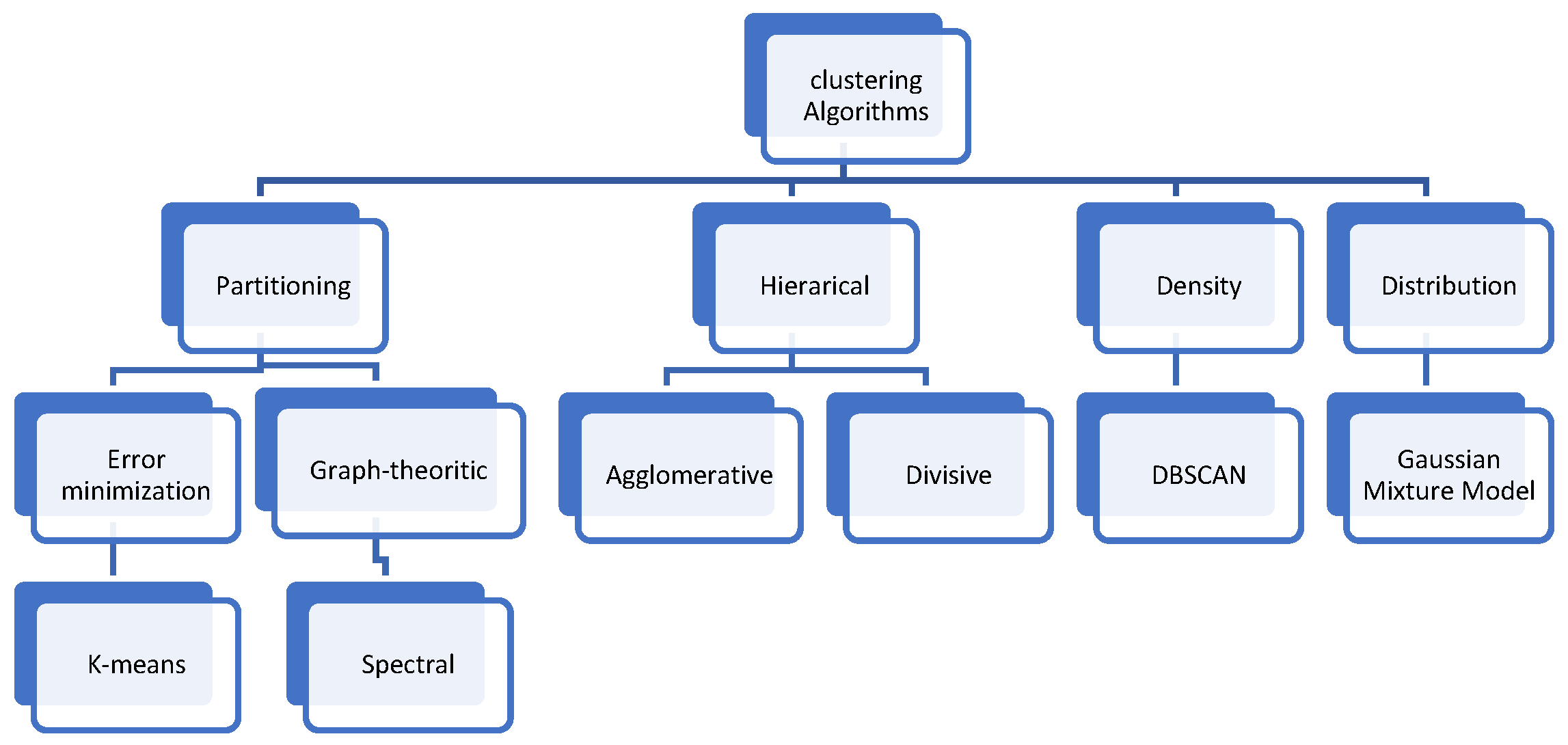
2.1. Types of Clustering Methods

Data clustering is an important issue in data mining [13] that can be divided into two groups: soft and hard [14]. Soft clustering means overlapping clustering, such as fuzzy clustering, where any data point may belong to more than one cluster with different membership grades. The other clustering, hard clustering, is exclusive clustering in which each data point exists in just one cluster [15].

From a different point of view, hierarchical and partitioning methods are the two main categories of clustering methods that were introduced in [16]. A hierarchical clustering method works by grouping data into a tree of clusters. In hierarchical clustering, the aim is to produce a hierarchical series of nested clusters. A diagram represents this hierarchy, which is an inverted tree that describes the order in which factors are merged (bottom-up view) or clusters are broken up (top-down view). On the other hand, the partitioning method was described in [13], which starts from an initial clustering and then moves data points from one cluster to another with a relocation method iteratively. There are two types of algorithms in this approach: error minimization algorithms and graph-theoretic clustering. The basic idea in error minimization algorithms is to determine clusters by minimizing a specified error criterion. The most famous algorithm in this area is k-means, which employs the sum of squared error (SSE) as an error criterion. The SSE measures the total squared Euclidean distance of instances to their representative values. However, k-means has some problems such as limiting to numeric attributes or being sensitive to initial centers of clusters. Therefore, some algorithms based on k-means such as k-prototype [17] or KHM [18] were proposed to overcome these problems. In addition, the k-medoids method was proposed, which is more robust than the k-means algorithm [19]. Graph-theoretic methods produce clusters via graphs. The famous algorithm in this method is based on the minimal spanning tree (MST) [20]. Another algorithm was proposed based on limited neighborhood sets [21].

From another perspective, clustering methods are divided into three main categories [13]: grid-based methods, density-based methods, and model-based clustering. The grid-based clustering methods use a multiresolution grid data structure to quantize object areas into a finite number of cells that form a grid structure, on which all the operations for clustering are implemented. Grid-based clustering uses dense grid cells to form clusters. [22]. Density-based clustering: The data points in the region separated by two clusters of low point density are considered as noise. DBSCAN is one of the most famous methods in this approach. The environment with a radius ϵ of a given object is known as the ϵ neighborhood of the object. If the ϵ neighborhood of the object includes at least a minimum number, MinPts, of objects, then it is called a core object [23].Model-based clustering (or distribution models): This method assumes a data model and applies an EM algorithm to find the most likely model components and the number of clusters [24].

2.2. Clustering APPLICATION in CPPs

Among the available clustering methods, k-means, spectral, and DBSCAN have been investigated more than others for solving CPPs. Therefore, we consider the proposed algorithms based on these methods.

Several solutions have been proposed based on the DBSCAN clustering method to appropriately locate the SDN controllers, as described in [25,26,27,28,29]. Since the method suggests the proper number of clusters, all of the proposed algorithms recommend a number of clusters, such as in [25], where the appropriate number of controllers is determined using silhouette analysis and gap statistics. However, one of the main disadvantages of the algorithm is that the value of the minimum number of objects should be defined in advance, which limits its ability to cluster datasets with high-density differences. Additionally, the neighborhood radius may not be suitable for all clusters, and this algorithm suffers from a high computational overhead.

In [26], the density-based controller placement (DBCP) method partitioned the given network using a density-based clustering method. This research considered CPPs with and without the capacity of controllers.

Clustering by fast search and find of density peaks (CFSFDP) proposed in [30] has been used in [27,28] to deal with the CPP. CFSFDP is a density-based clustering algorithm that requires fewer initial parameters and has more execution speed. However, it suffers from the need to experimentally preset the number of clusters.

The authors in [27] used a comprehensive consideration value according to [30], γ, which was calculated as the product of local density ($\rho$) and minimum distance (δ). However, two problems are identified with this definition. Firstly, the values of $\rho$ and δ may have different orders of magnitude, so they were normalized to ensure equal treatment. Secondly, nodes at different densities may have the same δ value, making it challenging to select the initial clustering center. To address this, the weight of δ was increased in low-density areas. The modified calculation equation for γ was presented as ${\gamma }_i={\rho }_i.{\delta }_i^\left(\frac{3}{4}\right)$.

A higher γ value indicates a higher likelihood of being a clustering center. The authors proposed a method to automatically determine the inflection point of γ, which corresponds to the transition from nonclustering centers to clustering centers. By analyzing the curve of γ values and finding the vertex of a folded line, the inflection point was identified. The optimal number of controllers was determined by counting the number of points with values greater than the inflection point γ value, and the locations of these points represented the deployment of clustering centers. The algorithm provided a step-by-step process for the selection of clustering centers.

The researchers in [28] utilized the idea of information entropy and a firefly algorithm for determining the local density and considered a point with the high density of switches as the cluster center. In the algorithm, the number and location of the controllers are discovered based on the jumping point in the decision graph.

The authors in [29] presented an improved density-based controller placement algorithm (DCPA) that enhances the efficiency of controller placement in a network. This algorithm achieves the required number of controllers by exploring candidate values of the radius and dividing the entire network into multiple subnetworks. Within each subnetwork, the controllers are deployed with the dual objective of minimizing the average propagation latency and the worst-case propagation latency between controllers and switches.

The spectral clustering method was used in [31,32,33,34,35] for CPP clustering. It is worth mentioning that the load-balancing parameter was considered in [31,32,35], and only [32,35] introduced algorithms for estimating the proper number of controllers. The authors in [32] utilized the structure of eigenvectors for the objective. In [33], first, the controllers were mapped into the row vector classification using spectral clustering, and then, using K-medoids algorithm, which is based on simulated annealing, the vectors were classified to achieve a flexible distribution of the controllers. The results in [34] demonstrated that the spectral algorithm outperforms K-median and K-center in terms of intercontroller latency. The problem was formulated for minimizing the controller cost, main costs, delays of switch–controller and intercontrollers, and main power cost in [35].

K-means was applied in [36,37,38] for solving a CPP in a SDN by paying attention to the delay between switches and controllers and load balancing. Only [38] among them considered intercontroller delay. It should be noted that the researchers in [37] also employed hierarchical clustering.

The authors in [39] mathematically formulated the placement of controllers as an optimization problem. The objectives of this problem were considered to minimize the controller response time, which refers to the delay between the SDN controller and assigned switches, as well as the control load (CL), intracluster delay (ICD), and intracluster throughput (ICT). To address this, they introduced a computationally efficient heuristic called deep-Q-network-based dynamic clustering and placement (DDCP). This heuristic utilized reinforcement and deep learning techniques to solve the optimization problem.

3. Basic Concepts

In this section, the basic concepts that will be used in this research are further explained.

3.1. K-Means Clustering

K-means clustering is a fast and commonly used technique due to its low iteration rates and ease of implementation. The k-means algorithm works by attempting to find the cluster centers (C₁, C₂, …, C_K) in a way that minimizes the total squared sum of distances between each data point “X_i” and its closest cluster center (C_j). However, the performance of k-means heavily depends on the initialization of the centers, which is a key issue with this algorithm. The algorithm establishes strong connections between data points and their closest cluster centers, resulting in cluster centers that do not leave the local range of data density. As the LAC algorithm is implemented via k-means, it still suffers from the issue of the random initialization of the centers. Thus, in this research, we optimized the algorithm by using KHM.

3.2. K-Harmonic Means

K-Harmonic means (KHM) was proposed by the authors in [18] as a new clustering method based on k-means. In this algorithm, the harmonic means are used instead of the Euclidean distance to solve the initialization problem of the KM algorithm.

The objective function of the KHM algorithm is named KHM, and it calculates the harmonic mean of the distance from each point to all centers. KHM investigates two functions, soft membership and weight. The weight function assigns a higher weight to data points that are far away from every center, defining the impact of each data point on computing new components of the cluster center. Parameter “ρ” is a user-defined input parameter in KHM, typically equal to or greater than 2. It influences the fuzziness of cluster assignments. A higher value of “ρ” results in smoother membership distributions and allows data points to have more evenly distributed memberships across multiple clusters. Conversely, a lower value of “ρ” leads to sharper cluster boundaries and more distinct memberships.

The algorithm continues until a predefined number of iterations is reached, or until the output of the KHM objective function does not change significantly.

3.3. Learning Automata

Learning automata [11] are probabilistic decision-making tools that iteratively adapt to the environment and learn the optimal action. A widespread type of learning automata is variable structure learning automata, which are defined by a quadruple [α, β, P, T], where:

• α = α₁, α₂, …, α_r is the set of actions where r is the number of actions.
• β is the reinforcement signals where, in a P-model environment, β ∈ [0, 1}.
• P = {p₁, p₂, …, p_r}} is the set of actions’ probability, P ∈{ 0, 1}.
• T is the learning algorithm where, in the n_th step, p(n + 1) = T[p(n), α(n), β(n)] is linear, if p(n + 1) is a linear function of p(n), or nonlinear if p(n + 1) is a nonlinear function of p(n).

In the n_th step of a linear learning algorithm, if the i_th selected action α_i(n) receives the reward reinforcement signal β(n) = 0, the corresponding probability vector of learning automaton, p(n + 1), is updated using 1. If it receives the penalty reinforcement signal β(n) = 1, the corresponding probability vector of learning automaton p(n + 1) is updated using 2 [40]:

$$p_j(n-1)=\left\{\begin{array}{c}{p}_j\left(n\right)+a\left(1-p_j\left(n\right)\right)\hspace{1em}\hspace{1em}j=i\\ p_j\left(n\right)\left(1-a\right)\hspace{1em}\hspace{1em}\forall j| j\ne i\end{array}\right.$$

(1)

$$p_j(n-1)=\left\{\begin{array}{c}{p}_j\left(n\right)-\left(1-b\right)\hspace{1em}\hspace{1em}j=i\\ \frac{b}{(r-1)}+\left(1-b\right)p_j\left(n\right)\hspace{1em}\hspace{1em}\forall j| j\ne i\end{array}\right.$$

(2)

where in Equations (1) and (2), a and b are learning parameters (reward and penalty parameters), and different values for a and b create different learning algorithms:

• If a = b, the learning algorithm will be of the linear reward penalty (LRP) type.
• If b = 0, the learning algorithm will be of the linear reward inaction (LRI) type.
• If a >> b (a is much larger than b), the learning algorithm will be of the reward epsilon penalty (LREP) type.

3.4. Learning-Automata-Based Clustering

In this form of clustering, each data point is equipped with the third type of learning automaton (LREP), and then, the learning automaton (LA) defines the membership status of the data point. The membership status of a data point in relation to a cluster is determined via “K-Means.” Therefore, this learning approach is based on the Euclidean distance between the data point and other data points within the cluster. The number of selectable actions for each learning automaton is equal to the number of clusters. After each selection, if the data point is assigned to the correct cluster, the selection is rewarded, and if not, it is penalized.

There are two reasons why the process of learning each data point was conducted using learning automata in this work:

• The input size: The input size is a function of the number of members and their attributes. It is necessary to mention that in the learning process of LA, the entirety of the given data are considered. It depends on the datasets.
• The cluster count: LA assign each datum to each cluster in during the learning process. The actions of the automata show the selection of a cluster for that particular member.

3.5. Software-Defined Networks and CPPs

Software-defined networks (SDNs) are a new network technology that is controlled centrally and intelligently. In this type of network, the management and tracing of packets are entirely the responsibility of the controlling part of it. The main issue of the network’s controlling plane occurs when the network size is large, as in this case, just one controller will not be able to cover the entire network. Therefore, the main challenge in this scenario is finding the right amount and location for the controllers. Clustering is one of the most reasonable viewpoints that can succeed in the complicated management process of large networks and can guarantee load balancing. Using the concept of clustering, a large network is divided into multiple subnetworks in a manner that there will be a controller for each subnetwork. Some matters such as the delay between controllers, load balancing, and reliability are also important considerations in addition to decreasing the delay between the switch and the controller.

4. LAC-KHM: The Proposed Algorithm

LAC-KHM is based on the LAC algorithm, in which each data point is equipped with a learning automaton (LA). The number of actions of each LA equals the number of clusters, and during the learning process, the LA specifies to which cluster its associated data point belongs. The action of each LA is chosen based on the action probability vector (APV). The LA’s decision is compared with the output of the k-means algorithm as a reinforcement signal. However, like k-means, LAC is sensitive to the proper selection of initial points. Therefore, in this research, LAC is improved through KHM, and the distance between data points and cluster centers is calculated with regard to the harmonic distance. The proposed algorithm, LAC-KHM, is formed based on three functions: select cluster, update probability, and calculate accuracy. The LAC-KHM algorithm is shown in Algorithm 1. It is noted that the cluster centers themselves are also updated based on the harmonic distance.

Algorithm 1: LAC-KHM algorithm

This algorithm has three functions with input and output parameters, and operations that follow:   Select Cluster: in fact, during rounds this function specifies to which cluster the data point belongs. It is noted that initially all actions in APV have the same probability. Input parameters: Membership_cluster, probability, num_cluster, num_data Output parameter: Membership_cluster Membership_cluster = Function Select_cluster (membership_cluster, probability, num_cluster, num_data)   Update probability: This function updates the APV using learning rule LRP based on the received reinforcement signal. In fact, with each execution, the probability of the selected action is either decreased or increased based on the harmonic distance between data points and cluster centers. Input parameters: membership_cluster, probability, num_cluster, position _of_data, signal, alpha, beta Output parameter: Probability Probability = Function Update_probability (membership_cluster, probability, num_cluster, position _of_data, signal, alpha, beta) Calculate accuracy: This function evaluates the accuracy of the algorithm, demonstrating how closely it matches the expected results. Input parameters: obtained_result, expected_result, num_cluster Output parameter: Accuracy Accuracy = Function Calculate accuracy (obtained_result, expected_result, num_cluster) After initializing parameters, the algorithm keeps on running until output of KHM objective function changes significantly.   Initialize parameters (x, y, until, n, k, d, numaction, probability, a, mask, signal, random centers) Membership_cluster = Function Select_cluster (membership_cluster, probability, num_cluster, num_data)    while (KHM changes significantly), do       for all data points, do             Call select-action Function (action= actionselection((action, probability, numactions, n))          end for          for all data points do            Calculate Membership of data (m function in KHM)    Calculate Weights of data (w function in KHM)    Calculate new_centers according to their Membership and Weights          end for          Calculate KHM      # Compute reinforcement signal          for all data points do    if actioni==clusteri :       signali=0    else       signali=1          for all data points do             Membership_cluster = Function Select_cluster (membership_cluster, probability, num_cluster, num_data)             Compute result (feedback of environment)          end for           # Update probability vector         for all data points do              Call Probability (probability = probabilityupdate(action, probability, numactions, n, signal, alpha, beta))          end for end while

5. CLAC-KHM: Customized LAC-KHM for CCP

Clustering algorithms have been applied in various scenarios, including solving the CPP. To solve the CPP, switches are mapped to data points and controllers to cluster centers. In most studies, the similarity criterion in clustering is the delay between the controller and the switch, which is essentially the distance between data points and centers in each cluster. It is also worth mentioning that the most practical algorithm is the one that considers other parameters, such as load balancing and intercontroller delay. Therefore, to solve the CPP, the LAC-KHM algorithm is customized to also consider load balancing and intercontroller distance, in addition to the distance between data points and centers. This means that the LA resident on each data point is rewarded not only when it reduces the distance between the data and cluster center, but also when it improves intercentral cluster and load balancing. As mentioned before, switches and controllers are placed in data points and cluster centers, respectively, and the network is partitioned based on this foundation.

Problem Formulation

SDN is a typical network comprising of controllers, switches, and links, which can be modeled as an undirected graph G = (V, E), where V represents a set of switches and E represents a set of links between the switches. In addition, n denotes the number of nodes in a given graph of switches, k denotes the number of controllers in the SDN, and C = {c₁,c₂,..,c_k} is a set of controllers. This algorithm divides the network into several subnetworks, with each cluster having a controller. Clustering the network is defined using SDN_i(V_i, E_i) as follows:

$$\bigcup _{i=1}^k{v}_i=V;\bigcup _{i=1}^k{E}_i=E$$

(3)

$${SDN}_i\cap {SDN}_j=\mathrm{\varnothing },\hspace{1em}\forall i\ne j,i,j\in k$$

(4)

$$\mathrm{S}({SDN}_i) =TRUE \forall i\in K$$

(5)

$$\mathrm{S}({SDN}_i\cap {SDN}_j)=\mathrm{FALSE},\hspace{1em}\forall i\ne j,i,jϵk$$

(6)

$${SDN}_i is a connected region \forall i\in k$$

(7)

Formula (3) implies that the network is covered with all formed subnetworks. Formula (4) demonstrates that there is no overlapping between subnetworks, and as mentioned, k denotes the number of controllers in the SDN. Formula (5) indicates that the highest similarity can be found between the members of the same cluster. Therefore, all of the switches can be assigned to one controller, and the lowest similarity is between the members of two different and separate clusters, which is demonstrated in Formula (6). Formula (7) indicates that all members of a subnetwork are connected with links. In this research, the similarities are intercontroller delay, controller/switch, and load balancing.

In this research, the objective function (OF) is defined as the following:

$$\mathrm{Objective} \mathrm{Function}=\alpha \ast l_{-}b-\beta \ast d_{S-C}-\mathsf{\gamma }\ast d_{C-C}$$

(8)

where $l_{-}b$ is denoted the load-balancing parameter. To calculate this parameter, we need to compute N_C, where the ideal range for the number of members in each cluster is defined as follows:

$$N\_C=\frac{n}{k}\pm \frac{n}{2k}$$

(9)

where n and k are the total number of switches and clusters, respectively. Consequently, if the number of members in a cluster is in the range of N_C, they are determined as True and if not, they are considered False.

Finally, l_b is the sum of clusters with the “True” tag, divided by k. The average delay between each switch and its related controller [41] and its normalized formula is demonstrated in (10) and (11).

$${\pi }^{avg(s-c)}=\frac{1}{n}\ast {\sum }_{v\in V}min d(v,c)$$

(10)

$$d_{s-c}(\mathrm{n}\mathrm{o}\mathrm{r}\mathrm{m}\mathrm{a}\mathrm{l}\mathrm{i}\mathrm{z}\mathrm{e}\mathrm{d})=\frac{{\pi }^{avg(s-c)}-\min ({\pi }^{avg\left(s-c\right)})}{\max ({\pi }^{avg\left(s-c\right)})-\min ({\pi }^{avg\left(s-c\right)})}$$

(11)

$${\pi }^{avg(c-c)}=\frac{1}{k}\ast \sum _{c_i,c_j\in C}\min d(C_i,C_j)$$

(12)

$$d_{c-c}(\mathrm{n}\mathrm{o}\mathrm{r}\mathrm{m}\mathrm{a}\mathrm{l}\mathrm{i}\mathrm{z}\mathrm{e}\mathrm{d})=\frac{{\pi }^{avg(C-C)}-\min \left({\pi }^{avg\left(C-C\right)}\right)}{\max \left({\pi }^{avg\left(C-\mathrm{C}\right)}\right)-\min \left({\pi }^{avg\left(C-C\right)}\right)}$$

(13)

Similarly, the intercontroller delay, which is calculated using “Dijkstra”, and its normalized format are illustrated in (12) and (13), respectively:

The coefficients α, β, and 𝛾 are still assumed to be in the range of [0, 1]. The values of l_b, d_S-C, and d_C-C depend on the specific context and units of measurement. These coefficients can be adjusted at any given time. The CLAC-KHM algorithm is demonstrated in Algorithm 2.

Algorithm 2: CLAC-KHM algorithm

Initialize parameters (x, y, n, k, d, k, numaction, probability, a, mask, signal, random centers) while (KHM changes significantly) do for all switches do       Call select-action Function end for for all switches do        Calculate Membership of data (m function in KHM)         Calculate Weights of data (w function in KHM)         Calculate new_centers according to their Membership and Weights         Calculate distance between controllers         for all clusters: do        Calculate objective function      end for      end for      Calculate KHM      for all of switches do        Compute result (feedback of environment)      end for      for all of LAs do      Call Probability      end for end while

6. Experimental Results

In this section, we evaluate LAC-KHM initially with seven datasets and then, the CLAC-KHM is compared with the three aforementioned algorithms on four topologies.

6.1. Performance Evaluation of LAC-KHM

In what follows, LAC-KHM’s efficiency is evaluated via comparisons with k-medians, k-medoids, k-means++, k-means, and standard LAC on seven different datasets, the features of which are displayed in

Table 1. The details of the datasets used in this research.

Dataset	Instances	Dimensions	Clusters	Membership_Cluster	LA Initial Prob
BCW	683	10	2	2	1/2
Sonar	208	60	2	2	1/2
CMC	1473	9	3	3	1/3
Hayes-Roth	132	5	3	3	1/3
Ionosphere	531	34	2	2	1/2
Sonar	208	60	2	2	1/2
Pima	768	8	2	2	1/2

. In addition, the input parameters of the functions in the LAC-KHM algorithm are also explained. Details of the dataset features and their initial values can be seen in this table as well. Additionally, the parameters of the LA are set according to those of [12].

Similarly, the results of checking the accuracy of the given algorithm compared to the rest are shown in

Table 2. Accuracies of the algorithms.

Dataset	K-Means	K-Means++	K-Medoid	LAC	LAC-KHM
BCW	0.50 ± 0.00	0.54 ± 0.00	0.50 ± 0.00	0.45 ± 0.00	0.50 ± 0.01
Sonar	0.49 ± 0.06	0.49 ± 0.06	0.49 ± 0.06	0.51 ± 0.04	0.54 ± 0.01
CMC	0.33 ± 0.04	0.32± 0.00	0.32 ± 0.00	0.34 ± 0.02	0.35 ± 0.01
Hayes-Roth	0.36 ± 0.03	0.41 ± 0.02	0.41 ± 0.02	0.42 ± 0.02	0.42 ± 0.02
Ionosphere	0.46 ± 0.03	0.48 ± 0.00	0.48 ± 0.00	0.48 ± 0.00	0.48 ± 0.01
Sonar	0.58 ± 0.21	0.78 ± 0.16	0.78 ± 0.16	0.90 ± 0.01	0.92 ± 0.11
Pima	0.49 ± 0.00	0.51 ± 0.00	0.51 ± 0.00	0.50 ± 0.00	0.52 ± 0.01

. As can be seen in this table, LAC-KHM achieves the best results.

6.2. Performance Evaluation of CLAC-KHM

In this section, CLAC-KHM is first compared to k-means, spectral, and LAC, and afterwards, they are all analyzed in a similar condition on four real internet zoo topologies on different scales. The initial values of the objective function in this study are shown in Equation (16):

$$\alpha =1,\beta =\frac{1}{2},\mathsf{\gamma }=\frac{1}{2}$$

(14)

Due to the fact that KHM is based on reducing the distance between the center and the points, and load balancing is another factor that relatively guarantees fault tolerance, α is set to 2.

Table 3. Symbols of the paper.

Parameter_Symbol	Explanation
α(LA)	Actions
β(LA)	Reinforcement signal
P	Action’s probability
T	The learning algorithm
a	Reward parameter
b	Penalty parameter
V	Set of switches
E	Set of links
L_B	Load-balancing coefficient
$d(v,c)$	Delay between switches and controller
$d(c,c)$	Delay between controllers
α(OF)	Coefficient of load balancing
β(OF)	Coefficient of delay between switches and their related controller
$\mathsf{\gamma }$(OF)	Coefficient of delay between controllers
n	Number of the switches
k	Number of the controllers
$N\_C$	Number of members in each cluster
${\pi }^{avg(s-c)}$	The average delay between each switch and its related controller
${\pi }^{avg(c-c)}$	The average delay between controllers
$d_{s-c}$	Normalization of ${\pi }^{avg(s-c)}$
$d_{c-c}$	Normalization of ${\pi }^{avg(c-c)}$

shows the details of the topologies used in this research. In [42], it is noted that some nodes have no complete information about latitudes and longitudes. Hence, we ignore these nodes throughout our simulations. Table 3 demonstrates the symbols of the paper.

In this research, we calculated the harmonic distance by replacing the Euclidean distance with the haversine distance, which is more appropriate for real-life topologies. The haversine distance is the distance between two data points on a sphere using their latitude and longitude. Therefore, we consider the minimum-delay path between all data points using the haversine distance [43]. The haversine formula uses the central angle Ɵ between every two data points on a sphere as shown in Equation (17), where d and r are the distance and the sphere radius, respectively.

$$\theta =\frac{d}{r}$$

(15)

The haversine distance is calculated via the haversine function which equals hav(Ɵ) = sin2(Ɵ), in which we are given a direct calculation of the longitude and latitude of the two points, as elaborated below:

ℎ𝑎v(Ɵ) = ℎ𝑎𝑣(ɸ₂ − ɸ₁) + 𝑐𝑜𝑠(ɸ₁)𝑐𝑜𝑠(ɸ₂)ℎ𝑎𝑣(𝜆₂ − 𝜆₁)

(16)

To solve for the distance d, we apply the archaversine (inverse haversine) to h = hav(θ) or use the arcsine (inverse sine) function:

$$d=r\ast archav\left(h\right)=2\ast r\ast aresin\left(\sqrt{h}\right)=$$

(17)

$$2\ast r\ast \mathrm{a}rcsin\sqrt{hav\left({\varnothing }_2-{\varnothing }_1\right)+\cos \left({\varnothing }_2\right)\cos \left({\varnothing }_1\right)hav({\lambda }_2-{\lambda }_1)}=$$

$$2\ast r\ast \arcsin (\sqrt{{sin}^2(\frac{{\varphi }_2-{\varphi }_1}{2})+\cos \left({\varphi }_1\right)\mathrm{c}\mathrm{o}\mathrm{s}({\varphi }_2){sin}^2(\frac{{\lambda }_2-{\lambda }_1}{2})})$$

The ɸ₁ and ɸ₂ are the latitudes and λ₁ and λ₂ are the longitudes of data_point₁ and data_point₂ in our function, respectively.

Since LAC is based on k-means, the CLAC-KHM algorithm is evaluated with standard k-means in addition to LAC. Spectral clustering is a method with roots in graph theory, whereas k-means, k-medoids, and k-median are methods based on the distance between the centers and data points. Therefore, they are different from spectral. That is why we also compared CLAC-KHM with the spectral algorithm on four topologies (Dialtecom, Intellifiber, Iris, and Aarnet) with four different sizes.

Table 4. Features of the topologies.

Number of Nodes	Number of Switches	Number of Edges	Geographical Area	Geographical Location
Dial telecom	193	151	country	Czech Republic
Aarnet	19	24	country	Australia
Intellifiber	73	97	country	USA
Iris	51	64	region	Tennessee, USA

shows the topologies’ details studied throughout our evaluations [42].

Table 5. Results of CLAC-KHM with 4 topologies.

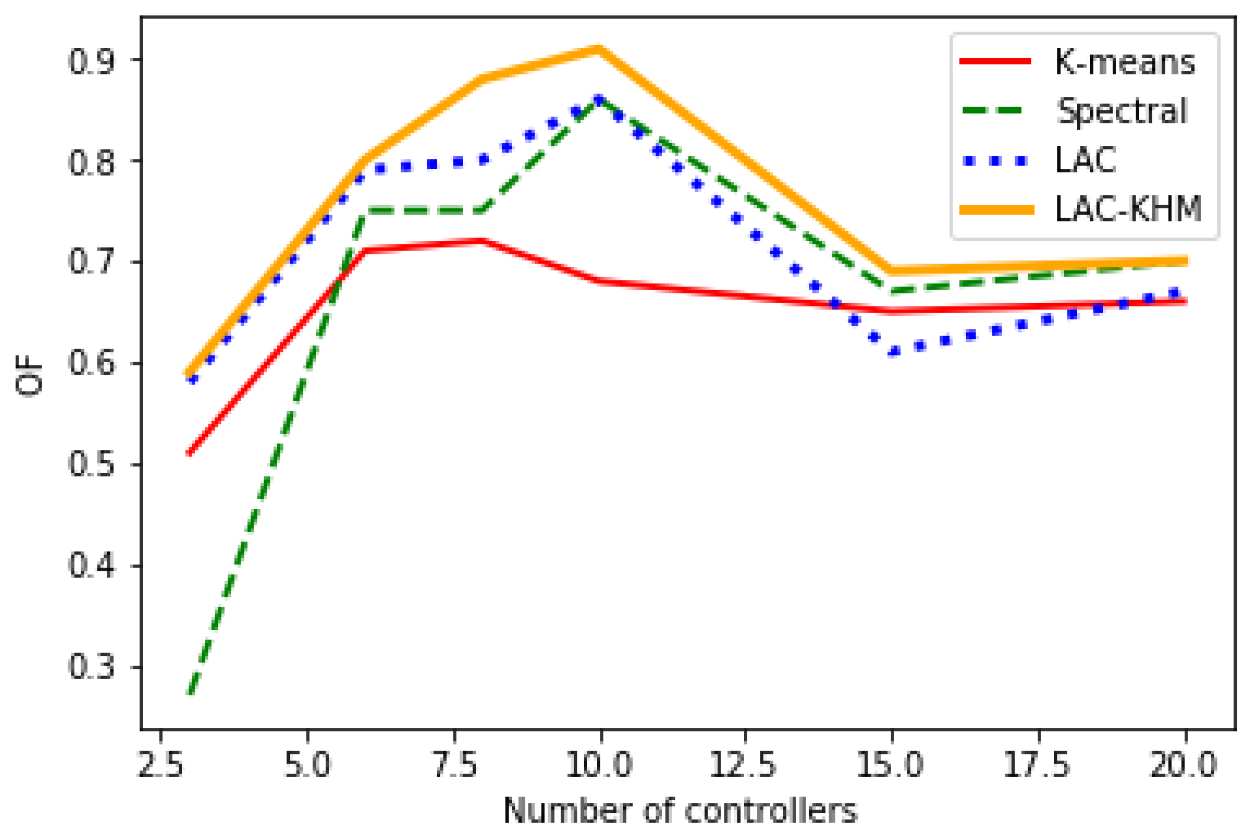
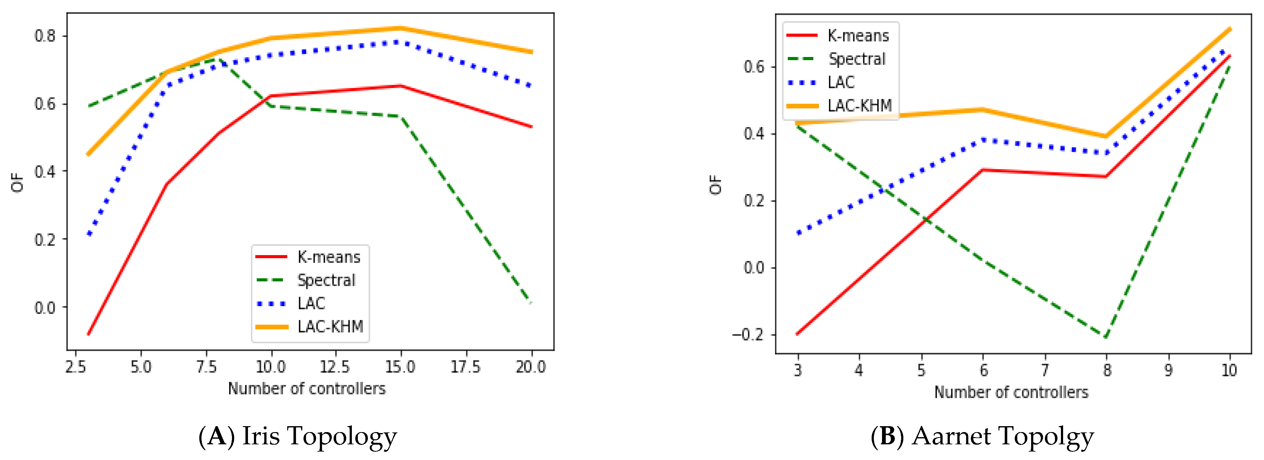
		Dial Telecom			Intellifiber			Iris			Aarnet
	NOC	S-C	C-C	OF	S-C	C-C	OF	S-C	C-C	OF	S-C	C-C	OF
K-means	3	18.77	0.96	0.51	21.94	3.37	0.52	7.22	1.67	-0.08	19.77	13.08	-0.2
	6	6.38	0.53	0.71	7.59	1.86	0.42	2.21	0.84	0.36	13.08	6.67	0.29
	8	3.9	0.45	0.72	4.78	1.64	0.47	1.35	0.67	0.51	1.65	5.48	0.27
	10	2.75	0.42	0.68	3.32	1.4	0.71	0.91	0.58	62	0.64	4.22	0.63
	15	1.48	0.32	0.65	1.65	1.18	0.45	0.41	0.44	0.65
	20	0.92	0.28	0.66	0.98	0.93	0.54	0.24	0.35	0.53
Spectral	3	20.57	1.09	0.27	22.35	3.41	0.58	7.78	1.25	0.59	23.57	9.47	0.42
	6	6.31	0.54	0.75	8.44	1.69	0.71	2.32	0.8	0.69	7.88	6.79	0.02
	8	3.95	0.46	0.75	5.28	1.41	0.7	1.4	0.61	0.73	3.76	3.59	-0.21
	10	2.87	0.41	86	3.35	1.34	0.59	0.96	0.53	0.59	3.7	3.29	0.6
	15	1.87	0.29	0.67	2.11	1.03	0.3	0.65	0.37	0.56
	20	1	0.25	0.7	1.41	0.9	0.37	0.54	0.27	0.01
LAC	3	17.78	0.95	0.58	20.14	3.01	0.53	6.72	1.37	0.21	17.77	12.08	0.1
	6	6.03	0.43	0.79	6.12	1.44	0.52	1.08	0.75	0.65	9.14	5.43	0.38
	8	3.54	0.4	0.8	4.78	1.64	0.58	0.64	0.57	0.71	1.65	5.46	0.34
	10	2.21	0.31	0.86	2.76	1.22	0.77	0.77	0.52	0.74	0.61	3.22	0.66
	15	1.23	0.26	0.61	1.43	1.02	0.6	0.38	0.38	0.78
	20	0.92	0.28	0.67	0.87	0.75	0.68	0.21	0.22	0.65
LAC-KHM	3	16.77	0.89	0.59	18.65	2.34	0.65	6.45	1.14	0.45	15.55	5.32	0.43
	6	6.13	0.39	0.8	5.24	1.12	0.74	0.99	0.68	0.69	7.23	5.88	0.47
	8	3.32	0.36	0.88	4.12	1.34	0.77	0.61	0.52	0.75	1.04	4.43	0.39
	10	1.97	0.29	0.91	2.06	1.01	0.81	0.74	0.5	0.79	0.54	3.12	0.71
	15	1.12	0.26	0.69	1.06	0.78	0.65	0.32	0.35	0.82
	20	0.88	0.21	0.7	0.66	0.63	0.75	0.17	0.18	0.75

presents the results. As mentioned previously, the Aarnet topology comprises 19 nodes, and for accommodating this topology, the number of controllers was examined within the range of 3 to 10. Consequently, in the table, you will observe a shaded area representing the number of controllers exceeding 10 for this particular topology.

The given values demonstrate that the delay between switches and controllers in k-means is less compared to that of spectral. However, the values of OF are not higher than spectral in all topologies with any number of controllers. These results determine that the CLAC-KHM achieves better results than the other algorithms as well. For the sake of a better explanation, the OF values are depicted for all algorithms in Figure 1, Figure 2 and Figure 3 for the four topologies.

In this study, it was observed that Dial_telecom is the largest topology, and the spectral algorithm achieved better results compared to k-means. However, as shown in Figure 2, LAC performed as well as the spectral algorithm. Nevertheless, it is noteworthy that CLAC-KHM achieved the best performance in this topology.

Figure 3 indicates the fact that the CLAC-KHM is the most efficient rather than the other representative algorithms. Meanwhile, it depicts that when there are a small number of controllers, the spectral clustering outperforms k-means in terms of OF, and contrarily, with increasing controller numbers, k-means has better results. It is worth bringing up the fact that they have no predictable behaviors in Intellifber.

As we can recognize in Figure 4A,B, the behavior of CLAC-KHM is similar to LAC and k-means while enjoying better performance on the Iris topology and Aarnet topology. In contrast, spectral clustering does not have a rather normal behavior.

From the attained results, it is concluded that the CLAC-KHM leads to better efficiency thanks to utilizing learning automata and KHM.

7. Conclusions and Future Works

In summary, the paper proposed two algorithms, LAC-KHM and CLAC-KHM, for solving the CPP in an SDN. LAC-KHM improved the LAC algorithm by incorporating the KHM method to avoid the sensitivity to the initialization of the algorithm. CLAC-KHM customized LAC-KHM for solving the CPP by considering the three main metrics, which were the distance between the controllers, the distance between controllers and switches, and load balancing. The proposed algorithms were evaluated on four different topologies, and the results showed that they outperformed k-means, spectral, and LAC algorithms. However, the proposed algorithms suffered from high computational complexity. This limitation arose due to the CLAC algorithm relying on the KHM algorithm, which entailed calculating the harmonic mean of distances between each data point and all centers for membership and weight functions. Consequently, this approach incurred a substantial computational burden. On the other hand, the CLA algorithm leveraged the k-means algorithm, which assigns data points to clusters based solely on their proximity to the assigned cluster, significantly reducing the computational complexity by avoiding calculations involving all clusters, which needs to be investigated in future works.

References

- Anil, K.; Jain, A.K.; Dubes, R.C. Algorithms for Clustering Data; Prentice-Hall: Upper Saddle River, NJ, USA, 1988. [Google Scholar]
- Liu, Q.; Kang, B.; Hua, Q.; Wen, Z.; Li, H. Visual Attention and Motion Estimation-Based Video Retargeting for Medical Data Security. Secur. Commun. Netw. 2022, 2022, 1343766. [Google Scholar] [CrossRef]
- Arora, N.; Singh, A.; Al-Dabagh, M.Z.N.; Maitra, S.K. A Novel Architecture for Diabetes Patients’ Prediction Using K-Means Clustering and SVM. Math. Probl. Eng. 2022, 2022, 4815521. [Google Scholar] [CrossRef]
- Granda Morales, L.F.; Valdiviezo-Diaz, P.; Reátegui, R.; Barba-Guaman, L. Drug Recommendation System for Diabetes Using a Collaborative Filtering and Clustering Approach: Development and Performance Evaluation. J. Med. Internet Res. 2022, 24, e37233. [Google Scholar] [CrossRef] [PubMed]
- Septiarini, A.; Hamdani, H.; Sari, S.U.; Hatta, H.R.; Puspitasari, N.; Hadikurniawati, W. Image Processing Techniques for Tomato Segmentation Applying K-Means Clustering and Edge Detection Approach. In Proceedings of the 2021 International Seminar on Machine Learning, Optimization, and Data Science (ISMODE), Jakarta, Indonesia, 29–30 January 2022; IEEE: Piscataway, NJ, USA, 2022; pp. 92–96. [Google Scholar]
- Avilov, M.; Shichkina, Y.; Kupriyanov, M. Using Clustering Methods of Anomalies and Neural Networks to Conduct Additional Diagnostics of a Computer Network. In Intelligent Distributed Computing XIV; Springer International Publishing: Cham, Switzerland, 2022; pp. 193–202. [Google Scholar]
- Yuan, L.; Chen, H.; Gong, J. Interactive Communication with Clustering Collaboration for Wireless Powered Communication Networks. Int. J. Distrib. Sens. Netw. 2022, 18, 15501477211069910. [Google Scholar] [CrossRef]
- Kumari, A.; Sairam, A.S. Controller Placement Problem in Software-Defined Networking: A Survey. Networks 2021, 78, 195–223. [Google Scholar] [CrossRef]
- Heller, B.; Sherwood, R.; McKeown, N. The Controller Placement Problem. ACM SIGCOMM Comput. Commun. Rev. 2012, 42, 473–478. [Google Scholar] [CrossRef]
- Ul Huque, M.T.I.; Si, W.; Jourjon, G.; Gramoli, V. Large-Scale Dynamic Controller Placement. IEEE Trans. Netw. Serv. Manag. 2017, 14, 63–76. [Google Scholar] [CrossRef]
- Narendra, K.S.; Thathachar, M.A. Learning Automata—A Survey. IEEE Trans. Syst. Man Cybern. 1974, 4, 323–334. [Google Scholar] [CrossRef]
- Hasanzadeh-Mofrad, M.; Rezvanian, A. Learning Automata Clustering. J. Comput. Sci. 2018, 24, 379–388. [Google Scholar] [CrossRef]
- Rokach, L.; Maimon, O. Clustering Methods. In Encyclopedia of Data Warehousing and Mining, 2nd ed.; Wang, J., Ed.; IGI Global: Hershey, PA, USA, 2009; pp. 254–258. [Google Scholar]
- Grover, N. A Study of Various Fuzzy Clustering Algorithms. Int. J. Eng. Res. 2014, 2, 177–181. [Google Scholar] [CrossRef]
- Bora, D.J.; Gupta, D.; Kumar, A. A Comparative Study between Fuzzy Clustering Algorithm and Hard Clustering Algorithm. arXiv 2014, arXiv:1404.6059. [Google Scholar]
- Reynolds, A.P.; Richards, G.; de la Iglesia, B.; Rayward-Smith, V.J. Clustering Rules: A Comparison of Partitioning and Hierarchical Clustering Algorithms. J. Math. Model. Algorithms 2006, 5, 475–504. [Google Scholar] [CrossRef]
- Huang, Z. Extensions to the k-Means Algorithm for Clustering Large Data Sets with Categorical Values. Data Min. Knowl. Discov. 1998, 2, 283–304. [Google Scholar] [CrossRef]
- Zhang, B.; Hsu, M.; Dayal, U. K-Harmonic Means-A Data Clustering Algorithm. Hewlett-Packard Labs Technical Report HPL-99-124. 1999. Available online: http://shiftleft.com/mirrors/www.hpl.hp.com/techreports/1999/HPL-1999-124.pdf (accessed on 20 June 2022).
- Kaufman, L.; Rousseeuw, P.J. Clustering by Means of Medoids. In Statistical Data Analysis Based on the L1-Norm and Related Methods; Dodge, Y., Ed.; North-Holland: Amsterdam, The Netherlands, 1987; pp. 405–416. [Google Scholar]
- Dussert, C.; Rasigni, G.; Rasigni, M.; Palmari, J.; Llebaria, A. Minimal Spanning Tree: A New Approach for Studying Order and Disorder. Phys. Rev. B 1986, 33, 3528–3531. [Google Scholar] [CrossRef] [PubMed]
- Urquhart, R. Graph Theoretical Clustering Based on Limited Neighbourhood Sets. Pattern Recognit. 1982, 15, 173–187. [Google Scholar] [CrossRef]
- Cheng, W.; Wang, W.; Batista, S. Grid-Based Clustering. Data 2018, 3, 25. [Google Scholar]
- Kriegel, H.P.; Kröger, P.; Sander, J.; Zimek, A. Density-Based Clustering. Wiley Interdiscip. Rev. Data Min. Knowl. Discov. 2011, 1, 231–240. [Google Scholar] [CrossRef]
- McNicholas, P.D. Model-Based Clustering. J. Classif. 2016, 33, 331–373. [Google Scholar] [CrossRef]
- Honarpazhooh, S. Controller Placement in Software-Defined Networking Using Silhouette Analysis and Gap Statistic. Turk. J. Comput. Math. Educ. 2021, 13, 4848–4863. [Google Scholar]
- Liao, J.; Sun, H.; Wang, J.; Qi, Q.; Li, K.; Li, T. Density Cluster Based Approach for Controller Placement Problem in Large-Scale Software Defined Networkings. Comput. Netw. 2017, 112, 24–35. [Google Scholar] [CrossRef]
- Xiaolan, H.; Muqing, W.; Weiyao, X. A Controller Placement Algorithm Based on Density Clustering in SDN. In Proceedings of the 2018 IEEE/CIC International Conference on Communications in China (ICCC), Beijing, China, 16–18 August 2018; pp. 184–189. [Google Scholar]
- Yujie, R.; Muqing, W.; Yiming, C. An Effective Controller Placement Algorithm Based on Clustering in SDN. In Proceedings of the 2020 IEEE 6th International Conference on Computer and Communications (ICCC), Chengdu, China, 11 December 2020; pp. 2294–2299. [Google Scholar]
- Chen, J.; Xiong, Y.; He, D. A Density-based Controller Placement Algorithm for Software Defined Networks. In Proceedings of the 2022 IEEE International Conferences on Internet of Things (iThings) and IEEE Green Computing & Communications (GreenCom) and IEEE Cyber, Physical & Social Computing (CPSCom) and IEEE Smart Data (SmartData) and IEEE Congress on Cybermatics (Cybermatics), Espoo, Finland, 22–25 August 2022; pp. 287–291. [Google Scholar]
- Rodriguez, A.; Laio, A. Clustering by Fast Search and Find of Density Peaks. Science 2014, 344, 1492–1496. [Google Scholar] [CrossRef]
- Xiao, P.; Qu, W.; Qi, H.; Li, Z.; Xu, Y. The SDN Controller Placement Problem for WAN. In Proceedings of the 2014 IEEE/CIC International Conference on Communications in China (ICCC), Shanghai, China, 13–15 October 2014; pp. 220–224. [Google Scholar]
- Xiao, P.; Li, Z.Y.; Guo, S.; Qi, H.; Qu, W.Y.; Yu, H.S. AK Self-Adaptive SDN Controller Placement for Wide Area Networks. Front. Inf. Technol. Electron. Eng. 2016, 17, 620–633. [Google Scholar] [CrossRef]
- Lu, J.; Zhen, Z.; Hu, T. Spectral Clustering Based Approach for Controller Placement Problem in Software Defined Networking. J. Phys. Conf. Ser. 2018, 1087, 042073. [Google Scholar] [CrossRef]
- Sahoo, K.S.; Sahoo, B.; Dash, R.; Tiwary, M. Solving Multi-Controller Placement Problem in Software Defined Network. In Proceedings of the 2016 International Conference on Information Technology (ICIT), Bhubaneswar, India, 21–24 December 2016; pp. 188–192. [Google Scholar]
- Zhao, Z.; Wu, B. Scalable SDN Architecture with Distributed Placement of Controllers for WAN. Concurr. Comput. Pract. Exp. 2017, 29, e4030. [Google Scholar] [CrossRef]
- Wang, G.; Zhao, Y.; Huang, J.; Duan, Q.; Li, J. A K-means-based network partition algorithm for controller placement in software defined network. In Proceedings of the 2016 IEEE International Conference on Communications (ICC), Kuala Lumpur, Malaysia, 22–27 May 2016; pp. 1–6. [Google Scholar]
- Kuang, H.; Qiu, Y.; Li, R.; Liu, X. A Hierarchical K-Means Algorithm for Controller Placement in SDN-Based WAN Architecture. Proceedings 2018, 2, 78. [Google Scholar]
- Zhu, L.; Chai, R.; Chen, Q. Control Plane Delay Minimization Based SDN Controller Placement Scheme. Proceedings 2017, 1, 536. [Google Scholar]
- Bouzidi, E.H.; Outtagarts, A.; Langar, R.; Boutaba, R. Dynamic clustering of software defined network switches and controller placement using deep reinforcement learning. Comput. Netw. 2022, 207, 108852. [Google Scholar] [CrossRef]
- Narendra, K.S.; Thathachar, M.A. Learning Automata: An Introduction. Entropy 2012, 14, 1415–1463. [Google Scholar]
- Torkamani-Azar, S.; Jahanshahi, M. A New GSO Based Method for SDN Controller Placement. Comput. Commun. 2020, 163, 91–108. [Google Scholar] [CrossRef]
- The Internet Topology Zoo. Available online: http://www.topology-zoo.org/ (accessed on 1 April 2023).
- Sminesh, C.N.; Kanaga, E.G.M.; Sreejish, A.G. A Multi-Controller Placement Strategy in Software Defined Networks Using Affinity Propagation. Int. J. Internet Technol. Secur. Trans. 2020, 10, 229–253. [Google Scholar] [CrossRef]