
Improvement of the Performance of Scattering Suppression and Absorbing Structure Depth Estimation on Transillumination Image by Deep Learning


Abstract
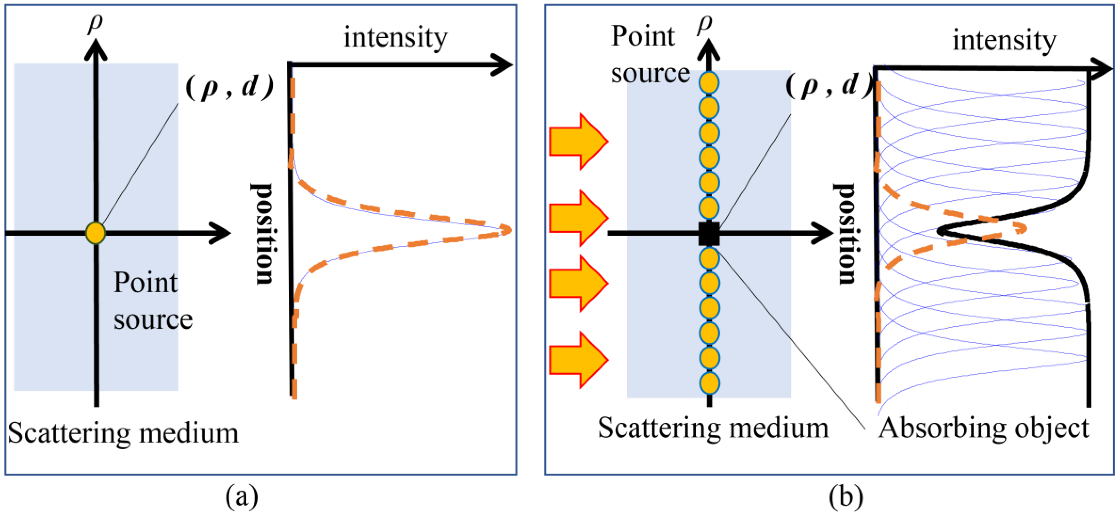
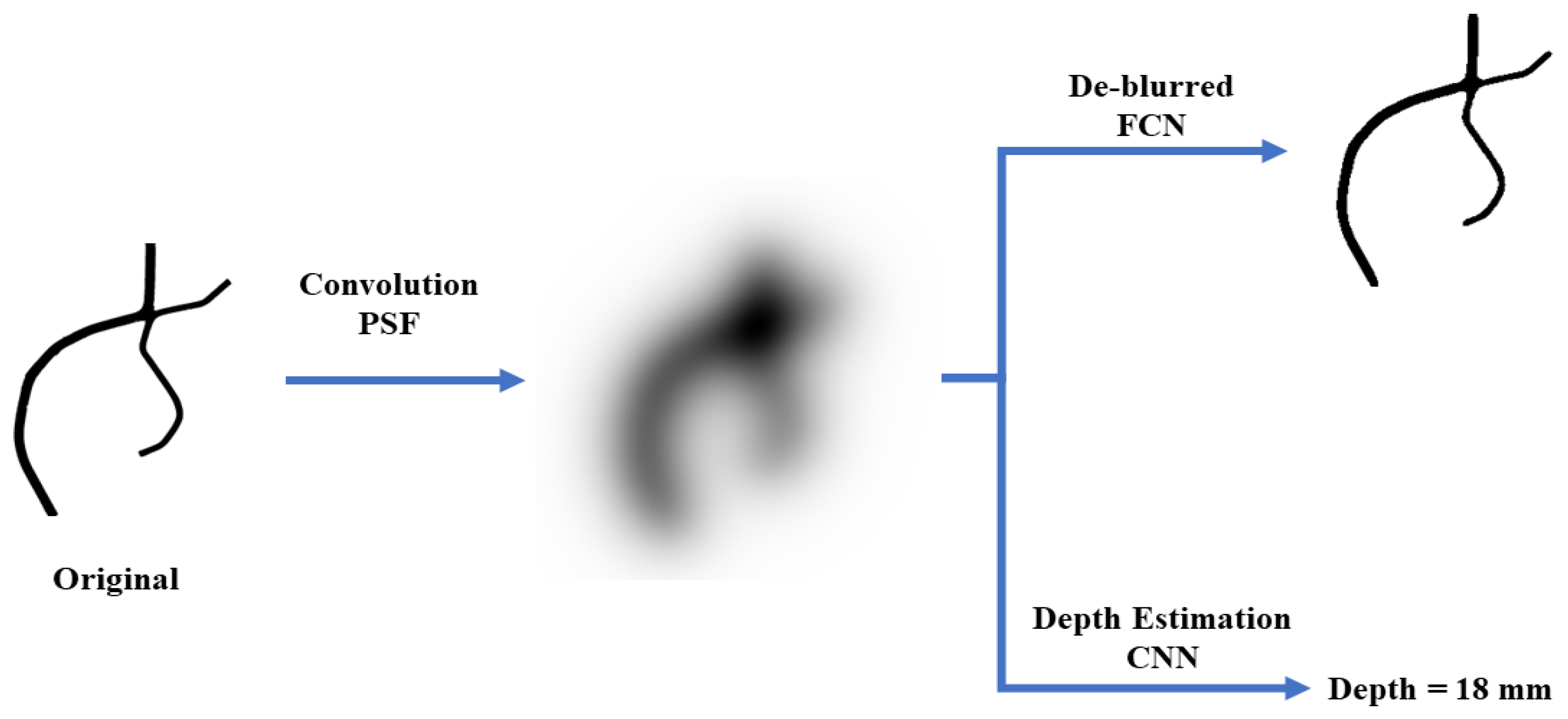
:1. Introduction
2. Materials and Methods
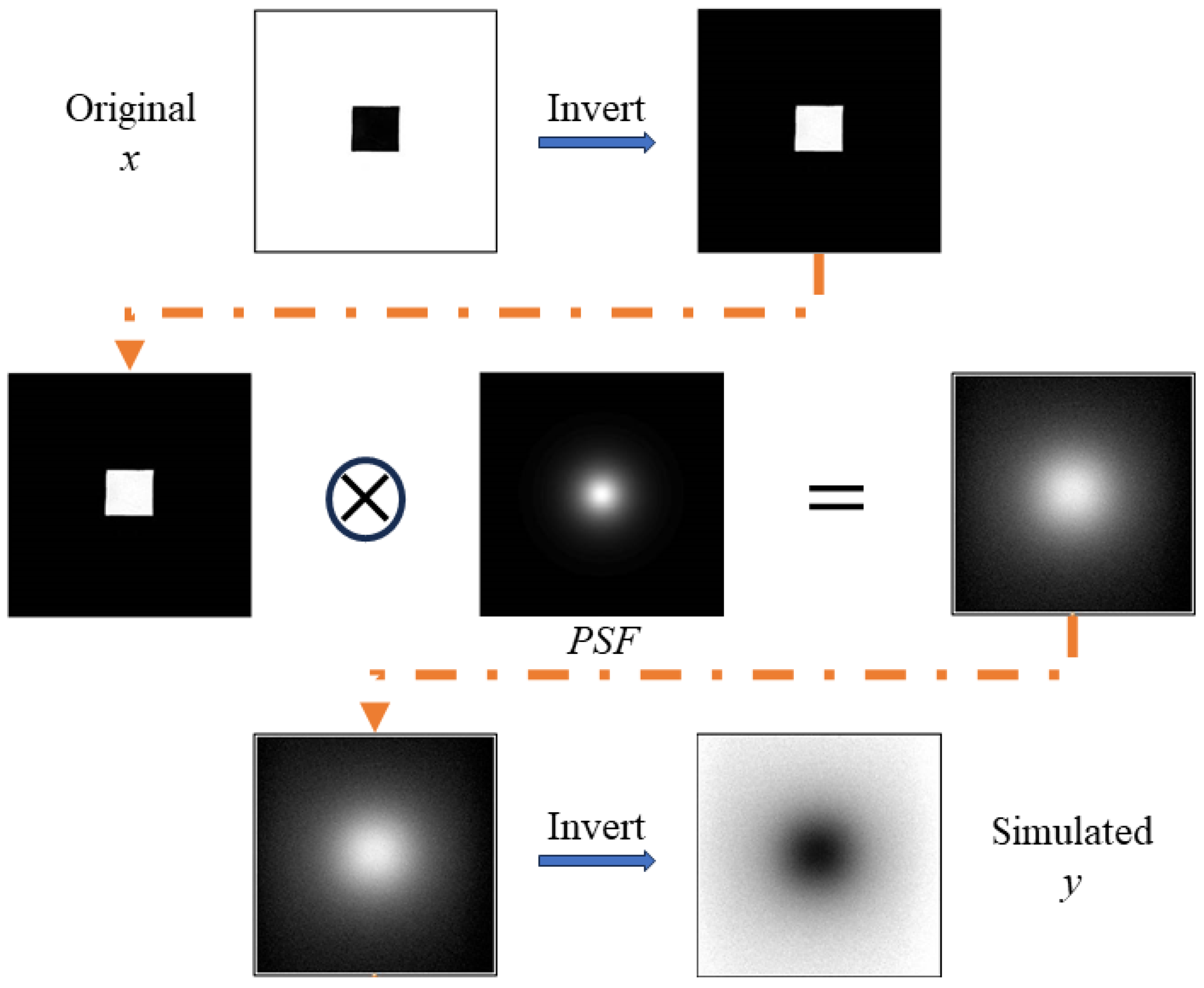
2.1. Data Preparation
- Empirical data: Experimental measurements of optical properties in specific tissue types at various wavelengths can serve as a foundation for determining the appropriate values. These measurements can come from the literature or new measurements conducted by the researchers themselves.
- Literature references: Previous studies often report ranges or specific values of and for similar tissue types. Researchers can use these references as a starting point and adjust the values based on their experimental setup.
- Theoretical models: There are established theoretical models that relate optical properties to tissue composition and structure. Researchers can leverage these models to estimate and based on the known components and concentrations in the tissue.
- Tissue variation: Different tissues exhibit different optical properties as a result of variations in cellular composition, structure, and pigmentation. Consequently, the specific tissue under investigation must be carefully considered when selecting and values.
- Wavelength Dependence: Optical properties can vary with the wavelengths of light. Researchers may choose and values that align with the wavelength range used in their experimental setup.
- Validation: Validating the chosen values involves comparing the simulation results with actual experimental observations. If the simulated outcomes closely match the experimental data, this provides confidence in the suitability of the parameter values.
- Sensitivity analysis: Researchers may conduct sensitivity analyses to assess how changes in and impact simulation results. This analysis helps to determine reasonable ranges for these parameters.
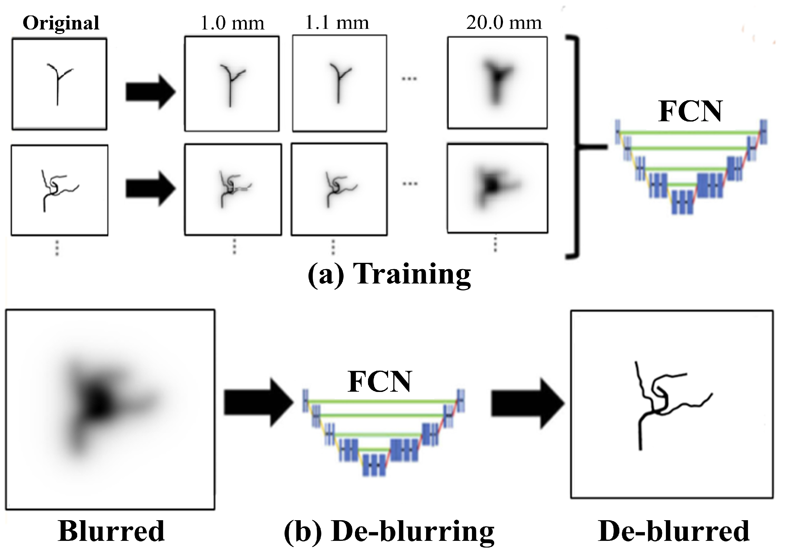
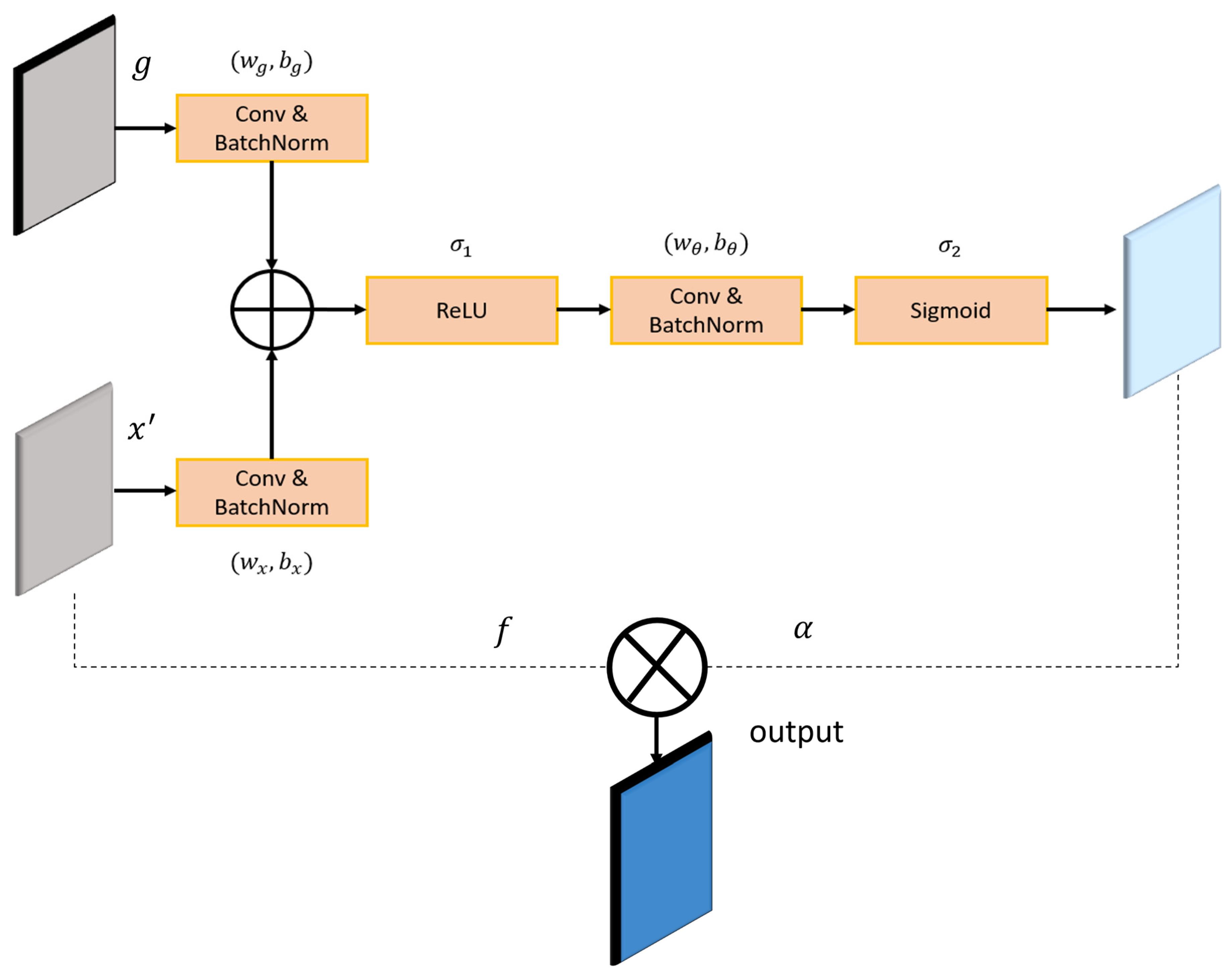
2.2. Image De-Blurring
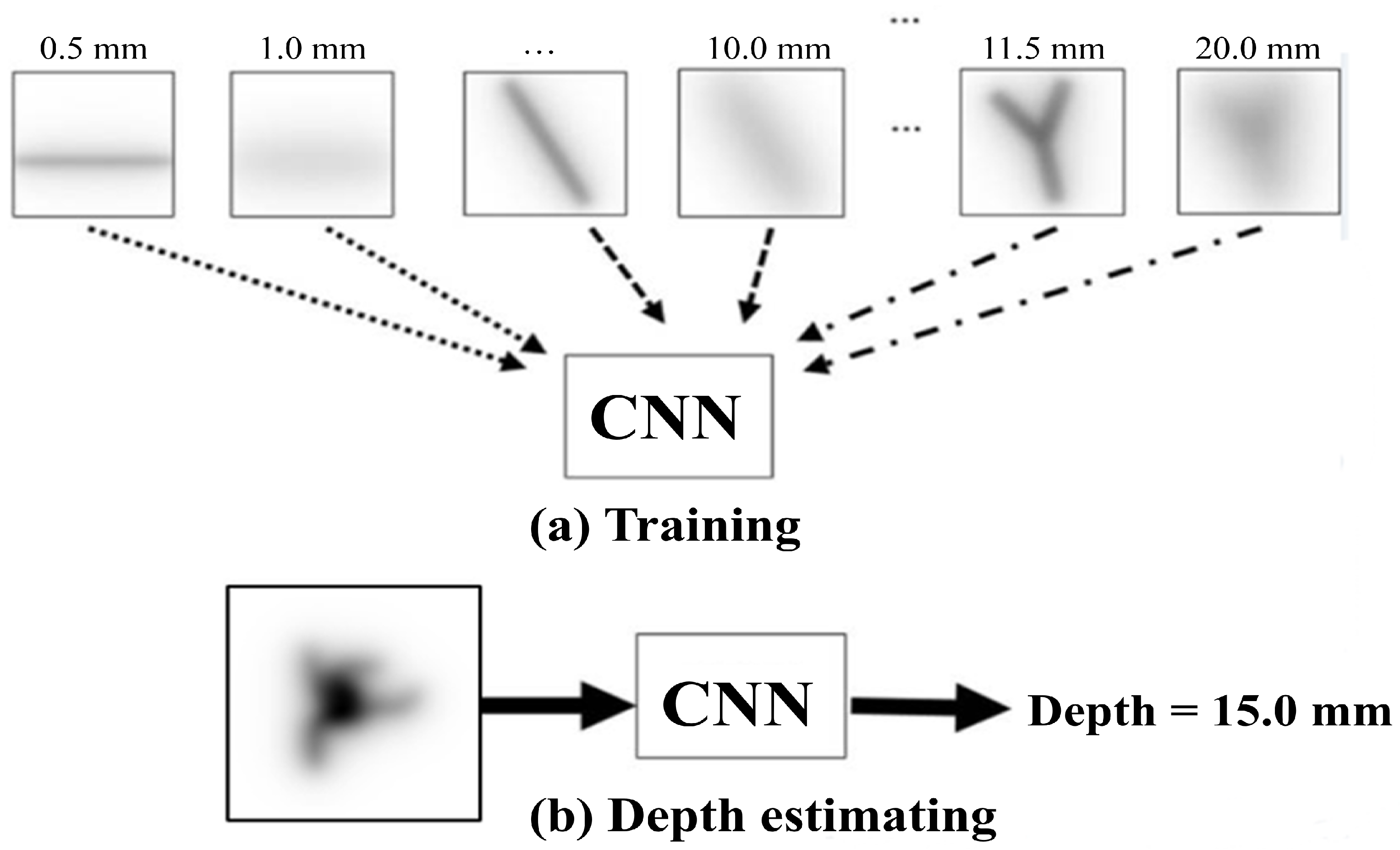
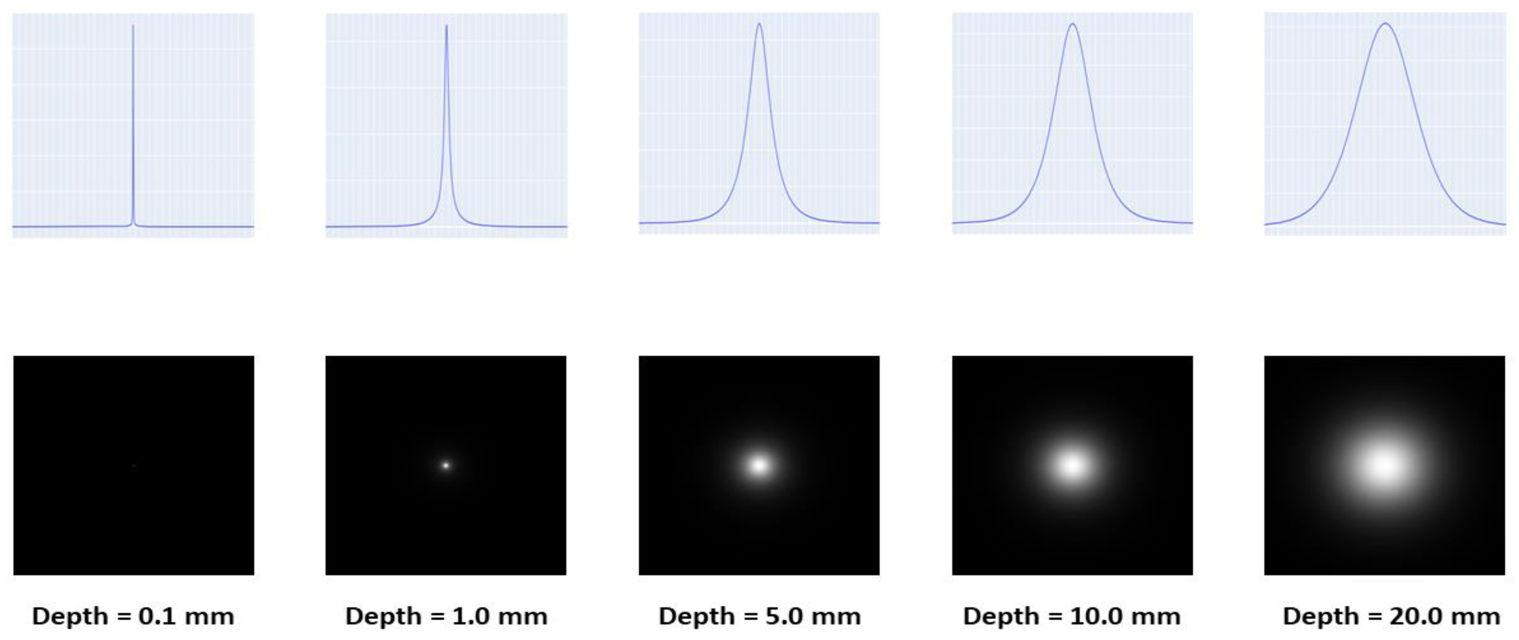
2.3. Depth Estimation
3. Metrics
4. Results and Discussion
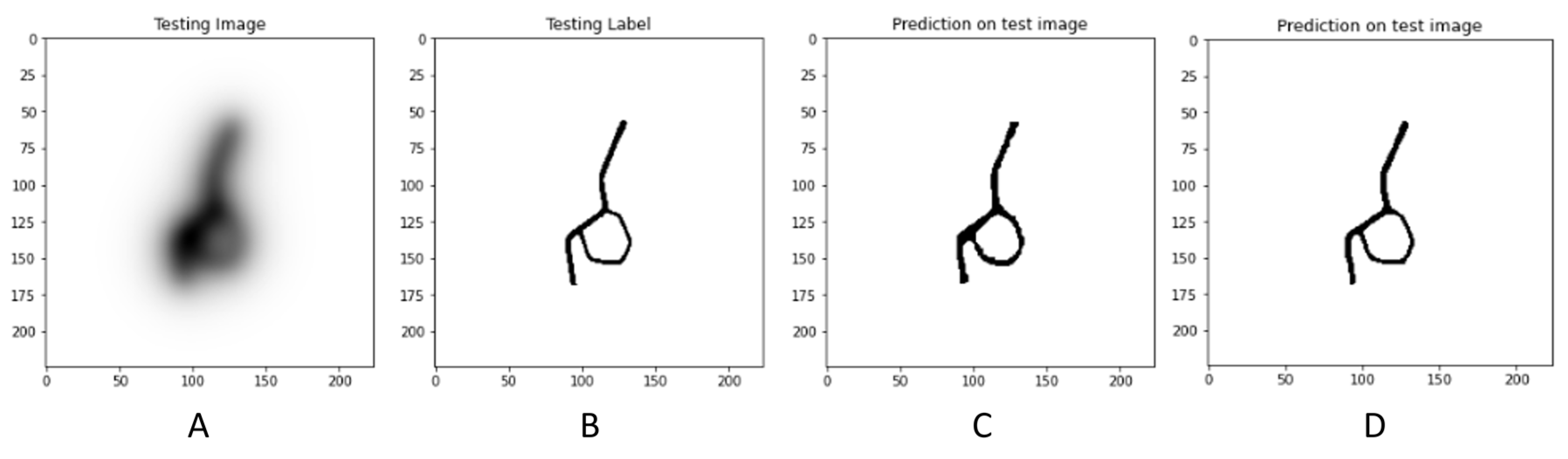
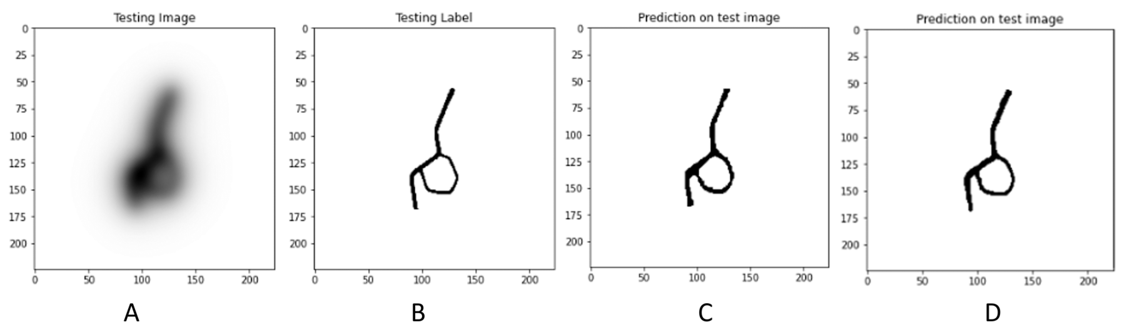
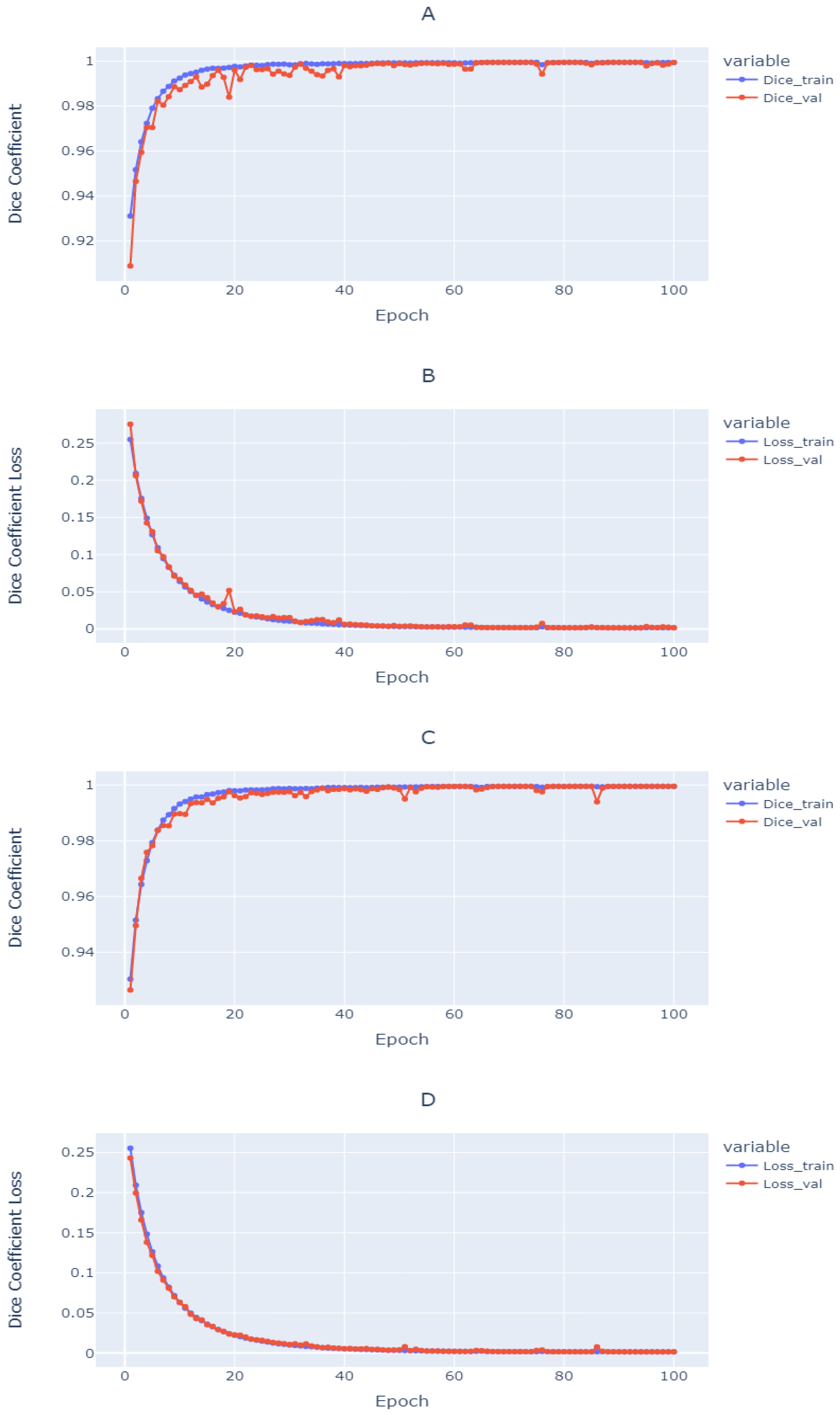
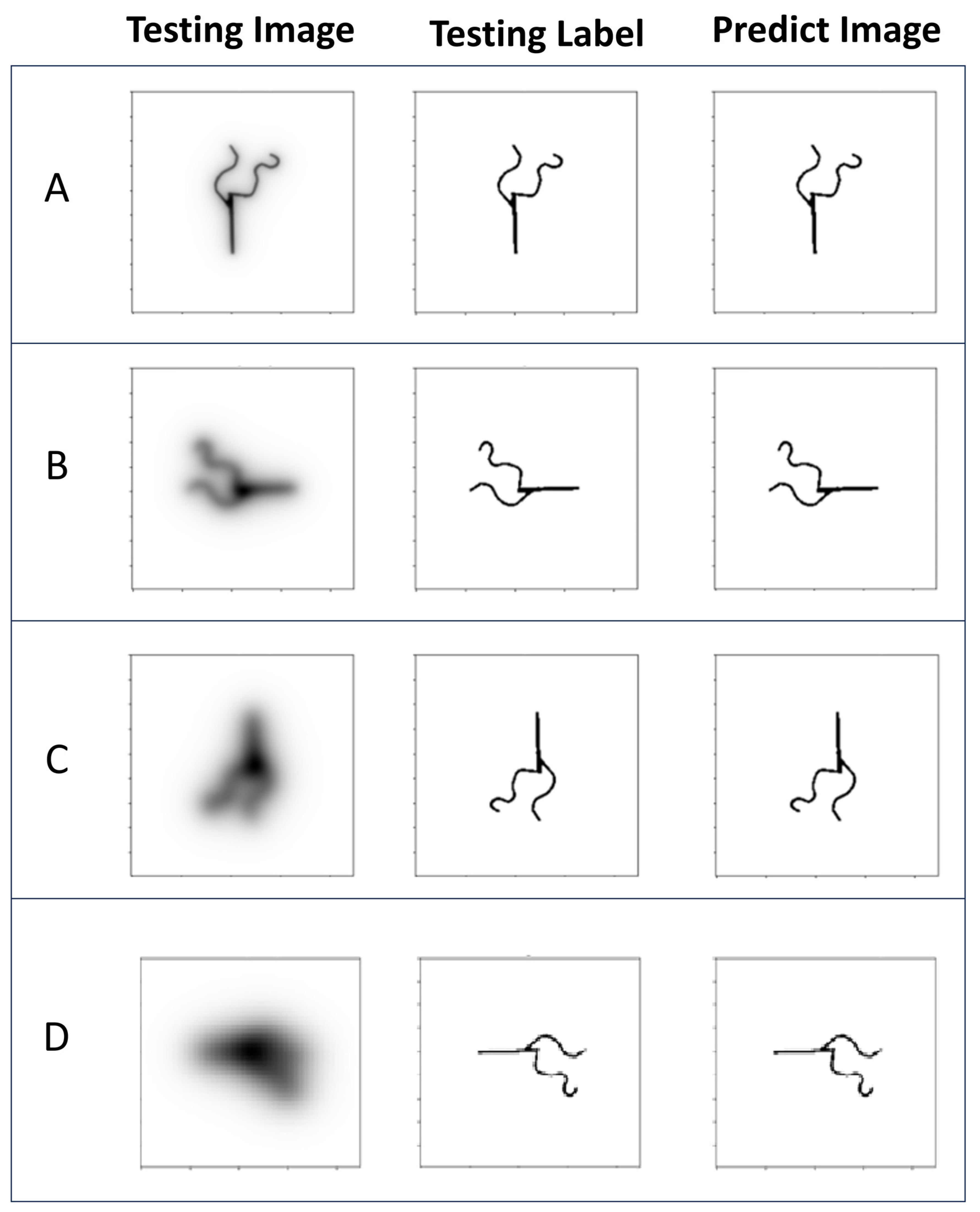
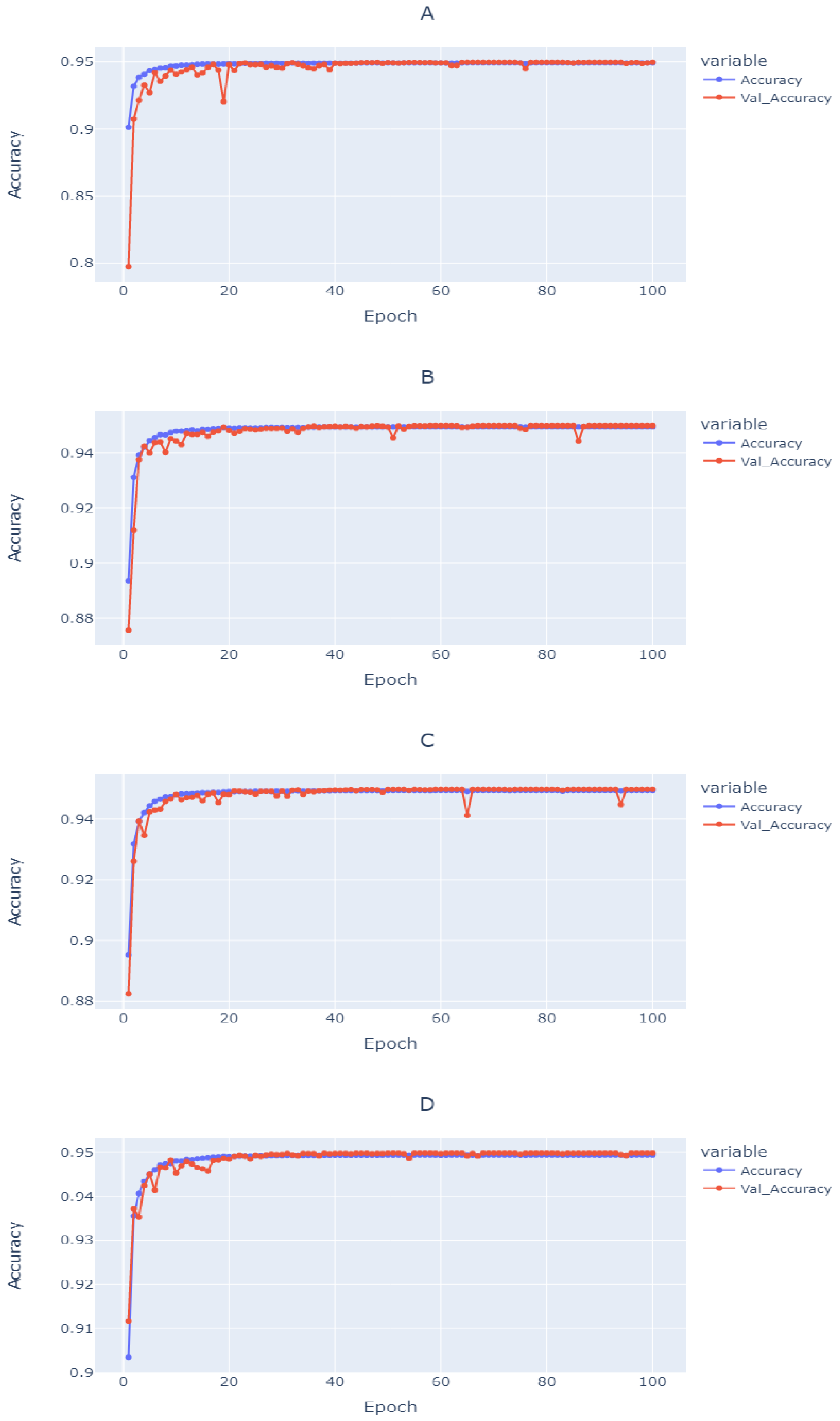
4.1. De-Blurring Image
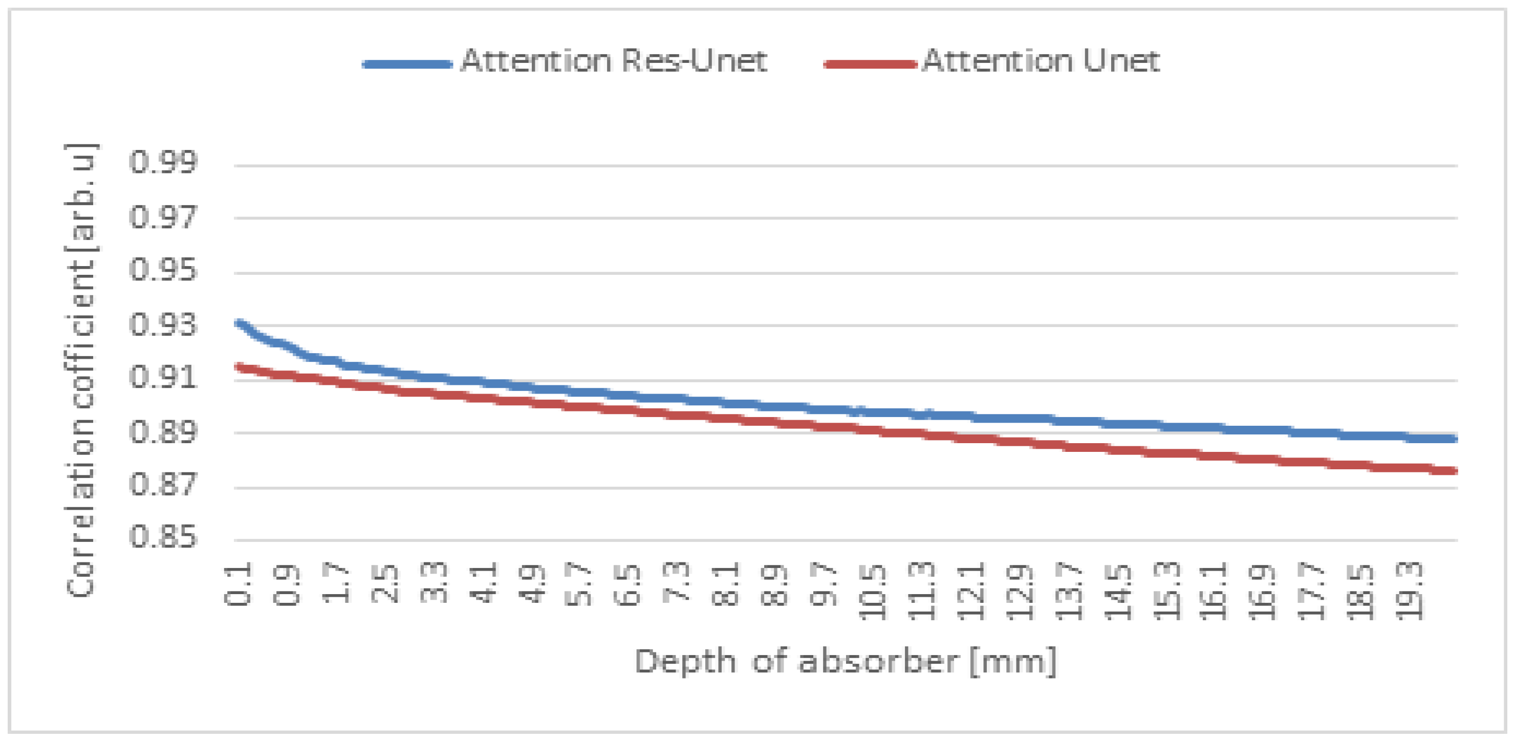
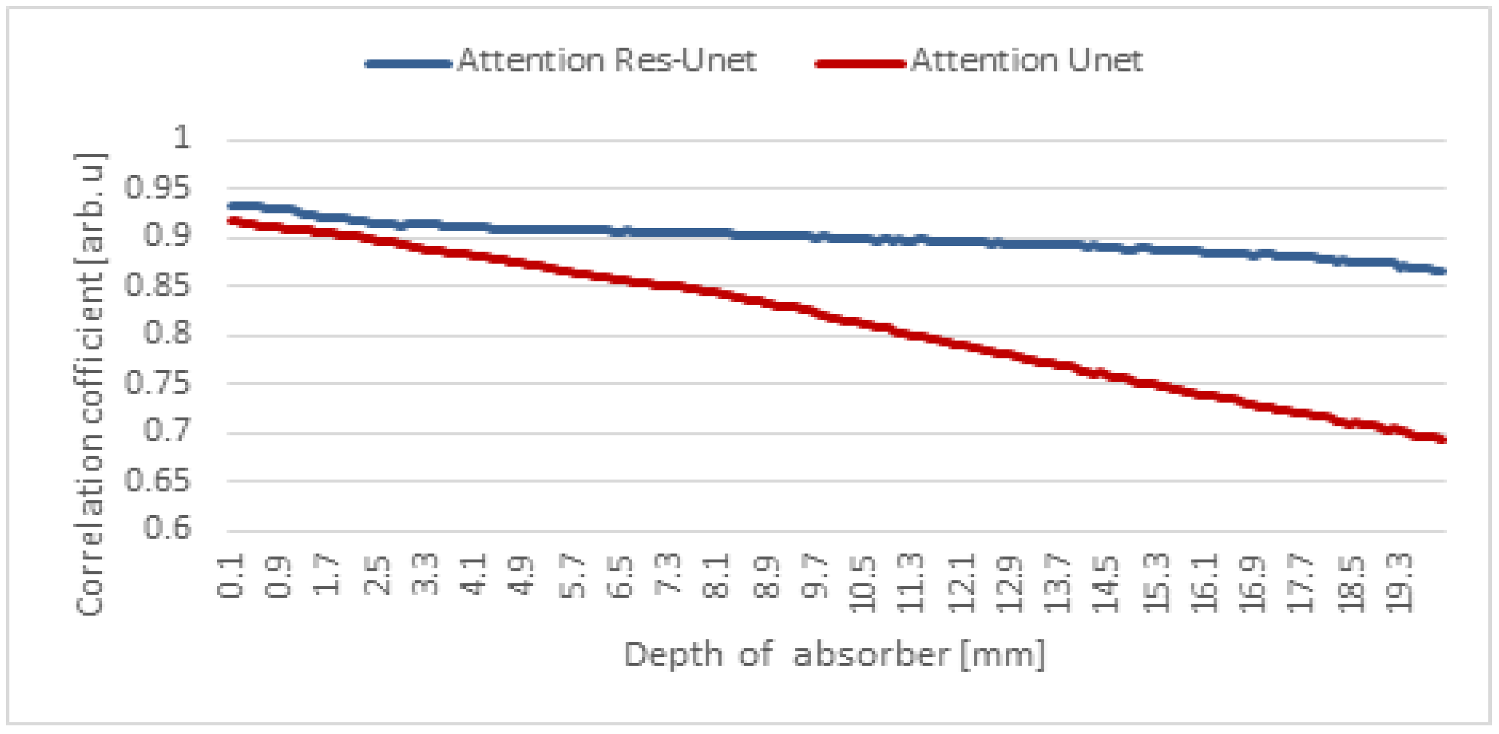
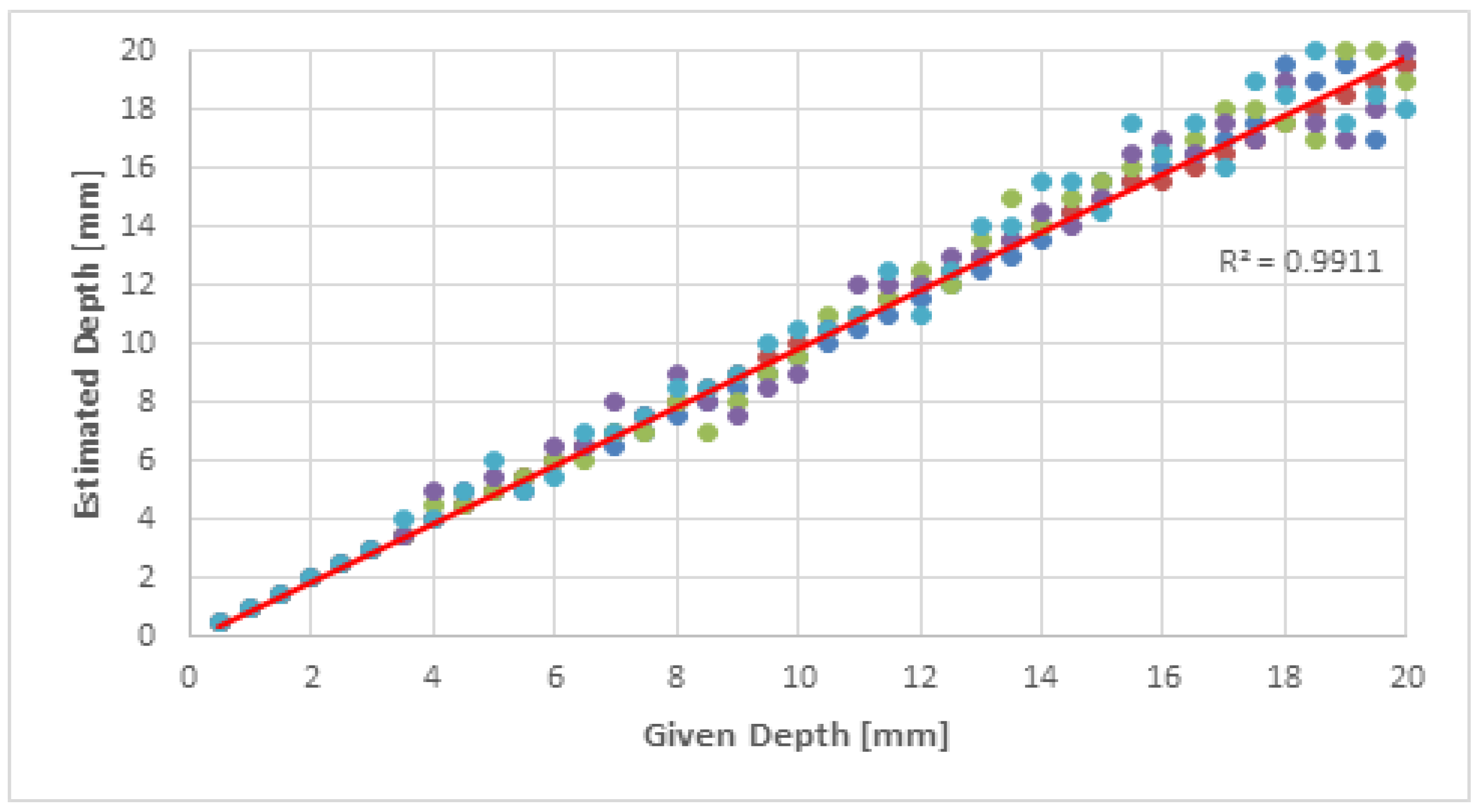
4.2. Depth Estimation
- Increased variability: By generating images from multiple angles, the dataset gains greater diversity. This variability acts as a defense against overfitting, ensuring that the model learns broader transferable features instead of memorizing specific training samples.
- Robustness to orientation: Real-world scenarios involve objects with varying orientations. Training the model on images spanning different orientations enhances its resilience to changes in object rotation.
- Feature extraction: Image rotation encourages the model to learn invariant features. It requires the model to emphasize features consistent across orientations, thus aiding in the extraction of pertinent and informative features for accurate depth estimation.
- Generalization: Exposure to an extensive array of angles equips the model with the ability to generalize its insights to novel orientations during inference.
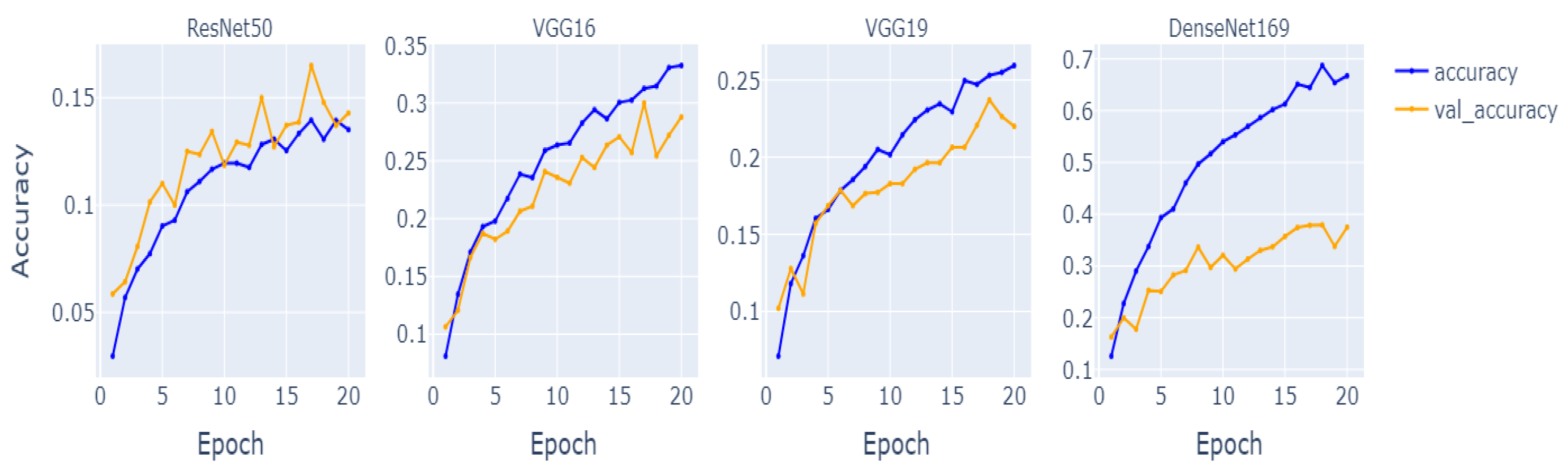
- All models attained substantial scores across evaluation metrics, indicating proficient performance in depth estimation.
- DenseNet169 secured the highest values in all metrics, followed by VGG16, VGG19, and ResNet50.
- The models demonstrated consistent alignment between accuracy, precision, recall, and F1 score, reflecting balanced performance in positive and negative classes.
- In particular, the application of angle rotation as an enhancement technique yielded notable improvements in the evaluation metrics compared to the previous experiment with the original dataset.
5. Conclusions
Author Contributions
Funding
Institutional Review Board Statement
Informed Consent Statement
Data Availability Statement
Acknowledgments
Conflicts of Interest
References
- Pan, C.T.; Francisco, M.D.; Yen, C.K.; Wang, S.Y.; Shiue, Y.L. Vein Pattern Locating Technology for Cannulation: A Review of the Low-Cost Vein Finder Prototypes Utilizing near Infrared (NIR) Light to Improve Peripheral Subcutaneous Vein Selection for Phlebotomy. Sensors 2019, 19, 3573. [Google Scholar] [CrossRef] [PubMed]
- Francisco, M.D.; Chen, W.F.; Pan, C.T.; Lin, M.C.; Wen, Z.H.; Liao, C.F.; Shiue, Y.L. Competitive Real-Time Near Infrared (NIR) Vein Finder Imaging Device to Improve Peripheral Subcutaneous Vein Selection in Venipuncture for Clinical Laboratory Testing. Micromachines 2021, 12, 373. [Google Scholar] [CrossRef] [PubMed]
- Frank, N.G.; David, W.; Samuel, D.; Martin, M.; Akwasi, A. Breast-i Is an Effective and Reliable Adjunct Screening Tool for Detecting Early Tumour Related Angiogenesis of Breast Cancers in Low Resource Sub-Saharan Countries. Int. J. Breast Cancer 2018, 2018, 2539056. [Google Scholar]
- Shiryazdi, S.M.; Kargar, S.; Nasaj, H.T.; Neamatzadeh, H.; Ghasemi, N. The accuracy of Breastlight in detection of breast lesions. Indian J. Cancer 2015, 52, 513–516. [Google Scholar] [PubMed]
- Tobisawa, N.; Namita, T.; Kato, Y.; Shimizu, K. Injection Assist System with Surface and Transillumination Images. In Proceedings of the 2011 5th International Conference on Bioinformatics and Biomedical Engineering, Wuhan, China, 13–15 May 2011; pp. 1–4. [Google Scholar]
- Shimizu, K.; Tochio, K.; Kato, Y. Improvement of transcutaneous fluorescent images with a depth-dependent point-spread function. Appl. Opt. 2005, 44, 2154–2161. [Google Scholar] [CrossRef] [PubMed]
- Tran, T.N.; Yamamoto, K.; Namita, T.; Kato, Y.; Shimizu, K. Three-dimensional transillumination image reconstruction for small animal with new scattering suppression technique. Biomed. Opt. Express 2014, 5, 1321–1335. [Google Scholar] [PubMed]
- Goh, C.M.; Subramaniam, R.; Saad, N.M.; Ali, S.A.; Meriaudeau, F. Subcutaneous veins depth measurement using diffuse reflectance image. Opt. Express 2017, 25, 25741–25759. [Google Scholar] [PubMed]
- Nguyen, N.A.D.; Van, T.N.P.; Yamamoto, K.; Nguyen, M.Q.; Tran, A.T.; Namita, T.; Shimizu, K.; Tran, T.N. Depth estimation of the absorbing structure in a slab turbid medium using point spread function. VNUHCM J. Eng. Technol. 2020, 3, SI10–SI21. [Google Scholar]
- Van, T.N.P.; Tran, T.N.; Inujima, H.; Shimizu, K. Three-dimensional imaging through turbid media using deep learning: NIR transillumination imaging of animal bodies. Biomed. Opt. Express 2021, 12, 2873–2887. [Google Scholar] [CrossRef] [PubMed]
- Shourav, M.K.; Choi, J.; Kim, J.K. Visualization of superficial vein dynamics in dorsal hand by near-infrared imaging in response to elevated local temperature. J. Biomed. Opt. 2021, 26, 026001. [Google Scholar] [CrossRef] [PubMed]
- Shimizu, K.; Xian, S.; Guo, J. Reconstructing a Deblurred 3D Structure in a Turbid Medium from a Single Blurred 2D Image—For Near-Infrared Transillumination Imaging of a Human Body. Sensors 2022, 22, 5747. [Google Scholar] [CrossRef] [PubMed]
- Mak, H.W.L.; Han, R.; Yin, H.H.F. Application of Variational AutoEncoder (VAE) Model and Image Processing Approaches in Game Design. Sensors 2023, 23, 3457. [Google Scholar] [CrossRef] [PubMed]
- Qiao, Q. Image Processing Technology Based on Machine Learning. In IEEE Consumer Electronics Magazine; IEEE: Piscataway, NJ, USA, 2022. [Google Scholar] [CrossRef]
- Patil, A. Image Recognition using Machine Learning. 2021. Available online: https://ssrn.com/abstract=3835625 (accessed on 30 August 2023).
- Oktay, O.; Jo Schlemper, J.; Folgoc, L.L.; Lee, M.; Heinrich, M.; Misawa, K.; Kensaku Mori, K.; McDonagh, S.; Hammerla, N.Y.; Kainz, B.; et al. Attention U-Net: Learning Where to Look for the Pancreas. arXiv 2018, arXiv:1804.03999. [Google Scholar]
- Maji, D.; Sigedar, P.; Singh, M. Attention Res-UNet with Guided Decoder for semantic segmentation of brain tumors. Biomed. Signal Process. Control 2022, 71, 103077. [Google Scholar] [CrossRef]
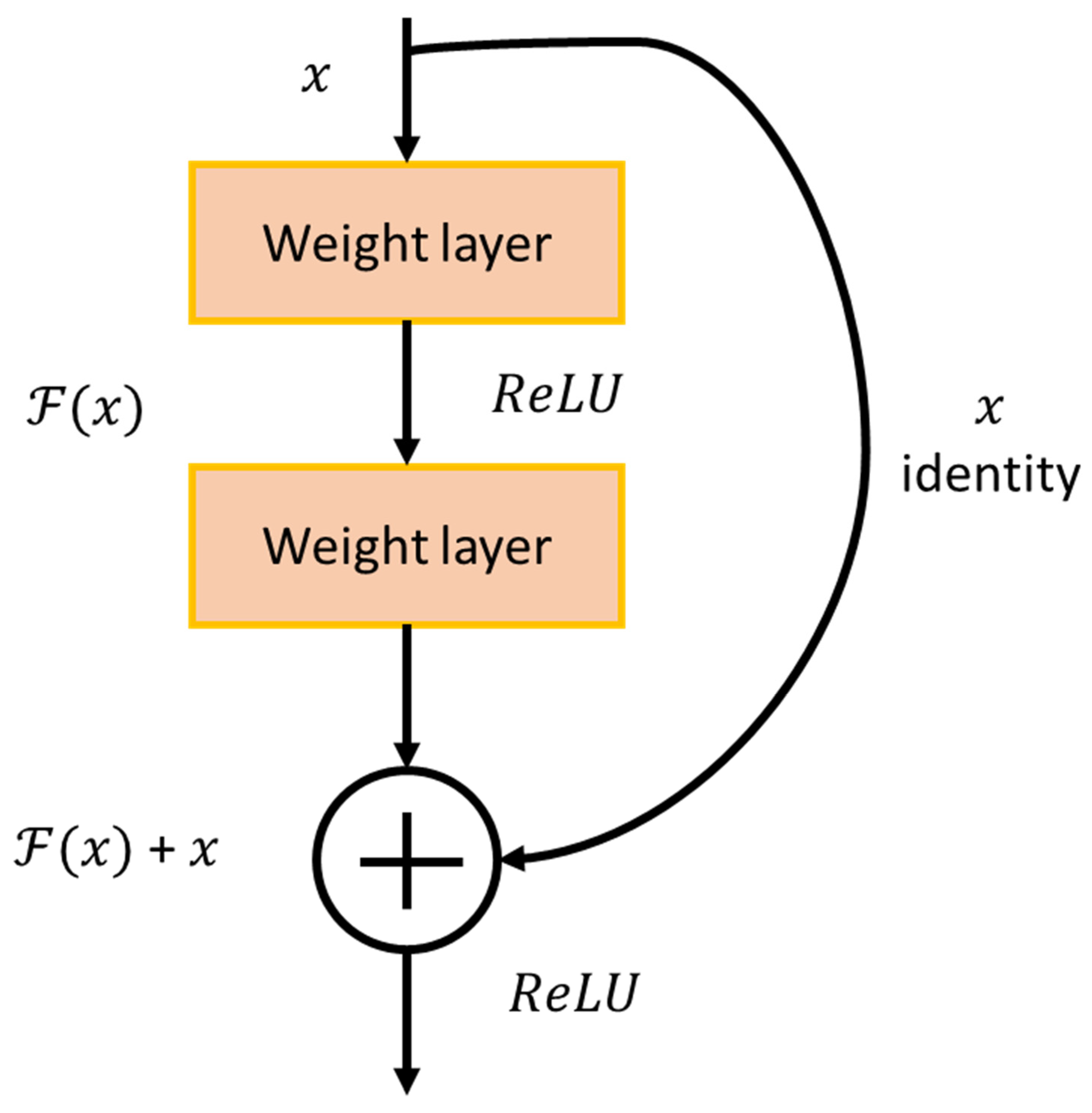
- He, K.M.; Zhang, X.Y.; Ren, S.Q.; Sun, J. Deep residual learning for image recognition. In Proceedings of the IEEE Conference on Computer Vision and Pattern Recognition, Las Vegas, NV, USA, 27–30 June 2016; pp. 770–778. [Google Scholar]
- Simonyan, K.; Zisserman, A. Very deep convolutional networks for large-scale image recognition. arXiv 2014, arXiv:1409.1556. [Google Scholar]
- Huang, G.; Liu, Z.; Van Der Maaten, L.; Weinberger, K.Q. Densely connected convolutional networks. In Proceedings of the IEEE Conference on Computer Vision and Pattern Recognition, Honolulu, HI, USA, 21–26 July 2017; pp. 4700–4708. [Google Scholar]
- Milletari, F.; Navab, N.; Ahmadi, S.A. V-Net: Fully convolutional neural networks for volumetric medical image segmentation. In Proceedings of the 2016 Fourth International Conference on 3D Vision (3DV), Stanford, CA, USA, 25–28 October 2016; pp. 565–571. [Google Scholar] [CrossRef]
- Rezatofighi, H.; Tsoi, N.; Gwak, J.; Sadeghian, A.; Reid, I.; Savarese, S. Generalized intersection over union: A metric and a loss for bounding box regression. In Proceedings of the IEEE/CVF Conference on Computer Vision and Pattern Recognition, Long Beach, CA, USA, 15–20 June 2019; pp. 658–666. [Google Scholar]
- Hossin, M.; Sulaiman, M.N. A review on evaluation metrics for data classification evaluations. Int. J. Data Min. Knowl. Manag. Process 2015, 5, 1–11. [Google Scholar]

| Model | Training | Validation | Testing | Total |
|---|---|---|---|---|
| De-blurred | 5600 | 1600 | 800 | 8000 |
| Estimate depth | 56,320 | 14,080 | 7040 | 70,400 |
| Parameters | De-Blurred | Depth Estimation |
|---|---|---|
| 1.0 mm−1 | 1.0 mm−1 | |
| 0.00536 mm−1 | 0.00536 mm−1 | |
| – | 0.1–20.0 mm | 0.5–20.0 mm |
| Step depth | 0.1 mm | 0.5 mm |
| Batch size | 8 | 32 |
| Learning rate | ||
| Epoch | 100 | 20 |
| Loss function | Dice-coef loss | Categorical Cross-entropy |
| Optimizer | Adam | Adam |
| Input shape | 256 × 256 × 1 | 224 × 224 × 1 |
| Model | Minimum | Maximum | Mean | Median | Std |
|---|---|---|---|---|---|
| Attention Unet | 0.931056 | 0.999487 | 0.996319 | 0.999195 | 0.009583 |
| Attention Res-UNet | 0.930391 | 0.999492 | 0.996443 | 0.999223 | 0.009603 |
| Model | Training Accuracy | Validation Accuracy |
|---|---|---|
| ResNet50 | 0.4312 | 0.3921 |
| VGG16 | 0.5124 | 0.4678 |
| VGG19 | 0.4894 | 0.4500 |
| DenseNet169 | 0.7323 | 0.6250 |
| Model | Accuracy | Precision | Recall | F1-Score |
|---|---|---|---|---|
| ResNet50 | 0.9212 | 0.9221 | 0.9212 | 0.9216 |
| VGG16 | 0.9324 | 0.9338 | 0.9324 | 0.9331 |
| VGG19 | 0.9294 | 0.9300 | 0.9294 | 0.9297 |
| DenseNet169 | 0.9523 | 0.9535 | 0.9523 | 0.9529 |
Disclaimer/Publisher’s Note: The statements, opinions and data contained in all publications are solely those of the individual author(s) and contributor(s) and not of MDPI and/or the editor(s). MDPI and/or the editor(s) disclaim responsibility for any injury to people or property resulting from any ideas, methods, instructions or products referred to in the content. |
© 2023 by the authors. Licensee MDPI, Basel, Switzerland. This article is an open access article distributed under the terms and conditions of the Creative Commons Attribution (CC BY) license (https://creativecommons.org/licenses/by/4.0/).
Share and Cite
Dang Nguyen, N.A.; Huynh, H.N.; Tran, T.N. Improvement of the Performance of Scattering Suppression and Absorbing Structure Depth Estimation on Transillumination Image by Deep Learning. Appl. Sci. 2023, 13, 10047. https://doi.org/10.3390/app131810047
Dang Nguyen NA, Huynh HN, Tran TN. Improvement of the Performance of Scattering Suppression and Absorbing Structure Depth Estimation on Transillumination Image by Deep Learning. Applied Sciences. 2023; 13(18):10047. https://doi.org/10.3390/app131810047
Chicago/Turabian StyleDang Nguyen, Ngoc An, Hoang Nhut Huynh, and Trung Nghia Tran. 2023. "Improvement of the Performance of Scattering Suppression and Absorbing Structure Depth Estimation on Transillumination Image by Deep Learning" Applied Sciences 13, no. 18: 10047. https://doi.org/10.3390/app131810047
APA StyleDang Nguyen, N. A., Huynh, H. N., & Tran, T. N. (2023). Improvement of the Performance of Scattering Suppression and Absorbing Structure Depth Estimation on Transillumination Image by Deep Learning. Applied Sciences, 13(18), 10047. https://doi.org/10.3390/app131810047