Expanded Scene Image Preprocessing Method for the Shack–Hartmann Wavefront Sensor

Abstract

Due to the influence of atmospheric turbulence, the detector, and background noise, the subaperture image of an extended scene Shack–Hartmann wavefront sensor will have a low signal-to-noise ratio, which will introduce errors to the offset estimation and reduce the accuracy of the slope measurement. To solve this problem, this paper proposes a cross-correlation subaperture image preprocessing method, which uses the generalized Anscombe transform to convert the Gauss–Poisson noise into Gaussian noise and introduces residual feedback on the basis of BM3D to achieve the efficient denoising of subaperture images. The simulation results show that compared with the three commonly used denoising algorithms, the proposed method improves the relative error of the subaperture offset calculation by 51.96% and the corresponding Zernike coefficient of distorted reconstruction wavefront by 85.56%, which realizes the improvement in the detection accuracy on the basis of effectively retaining image details.

1. Introduction

Advances in science and technology have greatly expanded the application of adaptive optics, leading to increased demands for real-time responsiveness and accuracy in wavefront detection. The Shack–Hartmann Wavefront Sensor (HWFS), comprising a microlens array and a CCD at its focal plane, has emerged as the dominant wavefront sensor due to its versatile features and capabilities [1,2]. For example, it has been well used in the visual performance and retinal imaging resolution of the human eye [3,4], optical imaging of scattering media [5,6], and biological studies [7].

To date, the research on Shack–Hartmann wavefront sensors has primarily focused on point-target imaging [8,9,10]. Various techniques have been employed to enhance the accuracy of the centroid extraction, including the windowed thresholded centroid of mass method [11], local adaptive thresholding [12,13], and the autocorrelation centroid of mass extraction [14]. These methods calculate the wavefront slopes for different subaperture ranges to achieve wavefront reconstruction. However, certain domains, such as solar telescopes, space-to-earth remote sensing, and other applications, face challenges in locating point targets within the field of view. Consequently, extended targets are introduced [15,16]. Extended target Shack–Hartmann wavefront sensors produce arrays of sub-images that exhibit similar content on the CCD. To prevent overlap between the sub-images, additional field-of-view diaphragms are required to limit the image size [17]. Wavefront phase errors cause shifts in the sub-images; thus, the accuracy of wavefront detection depends primarily on the accurate determination of the offset between each sub-image. Factors such as atmospheric turbulence and noise [18] contribute to a decrease in the signal-to-noise ratio, thereby diminishing the accuracy of wavefront detection [19].

In recent years, there has been significant interest, both domestically and internationally, in methods aimed at enhancing the accuracy of wavefront under low signal-to-noise ratios. Mao et al. proposed a method to estimate the noise error using multi-frame Shack–Hartmann photograms and their computed center-of-mass displacements, and the estimation error of this method can be less than 2% under the condition that the signal-to-noise ratio meets the normal operation of the Shack–Hartmann sensor [20]. Kong et al. developed a centroid of the mass estimator utilizing stream processing, which mitigates the impact of background and noise when the scene content is smaller than the subaperture field of view [21]. Anugu et al. proposed an algorithm based on the antisymmetric response of the bias to the subpixel position of the true centroid, effectively reducing the bias by a factor of approximately seven, albeit with twice the computational expenses compared to current mutual algorithms [22].

In order to enhance the accuracy of detection, we propose an image preprocessing method that involves reducing the noise in the sub-image array acquired from the CCD. The introduced Gaussian–Poisson noise is converted to Gaussian noise using the Generalized Anscombe transform (GAT) [23]. To handle the image noise, we utilize residual feedback for block-matching and 3D filtering (BM3D). Additionally, we perform offset computation using the normalized intercorrelation algorithm [24] to achieve wavefront reconstruction [25].

2. Methods

2.1. Principles of Wavefront Detection for Extended Target Shack–Hartmann Wavefront Sensors

Since extended targets are imaged against the same target, each subaperture image is virtually the same. When the incident wavefront is subjected to wavefront disruption, the position of the subaperture image is comparatively moved. The offset of the subaperture picture is determined by the mutual correlation method as a reference image when there is no distortion, and parabolic interpolation is carried out in the vicinity of its peak-maximum location to obtain subpixel level accuracy [26,27,28]. To locate the peak, the mutual correlation approach uses the normalized mutual correlation function as a criterion function for picture alignment. Equation (1) below illustrates the calculation for the normalized mutual correlation function:

$${\mathrm{r}}_{sr}(x_0,y_0)=\frac{{\displaystyle \sum _{x=1}^M}{\displaystyle \sum _{y=1}^M}{I}_s(x+x_0,y+y_0)I_r(x,y)}{\sqrt{{\displaystyle \sum _{x=1}^M}{\displaystyle \sum _{y=1}^M}{I}_s^2(x+x_0,y+y_0)\times {\displaystyle \sum _{x=1}^M}{\displaystyle \sum _{y=1}^M}{I}_r^2(x,y)}},$$

(1)

where the size of the reference image is $M\times M$ pixels, $I_r(x,y)$ and $I_s(x,y)$ denote the gray values of the reference image and the aberrated image at $(x,y)$, respectively, and $(x_0,y_0)$ is regarded as the offset of the subaperture image in both directions. The peak value of the cross-correlation function is obtained when the similarity between the subaperture images of the reference image and the distorted image is maximum.

The offsets of the subaperture images usually need to be interpolated to subpixel accuracy. The parabolic interpolation method adopted is shown in Equation (2):

$$\begin{array}{c}{x}_0={\mathrm{\Delta }}_x+\frac{0.5\left[C\left({\mathrm{\Delta }}_x-1,{\mathrm{\Delta }}_y\right)-C\left({\mathrm{\Delta }}_x+1,{\mathrm{\Delta }}_y\right)\right]}{C\left({\mathrm{\Delta }}_x-1,{\mathrm{\Delta }}_y\right)+C\left({\mathrm{\Delta }}_x+1,{\mathrm{\Delta }}_y\right)-2C\left({\mathrm{\Delta }}_x,{\mathrm{\Delta }}_y\right)}\hfill \\ y_0={\mathrm{\Delta }}_y+\frac{0.5\left[C\left({\mathrm{\Delta }}_x,{\mathrm{\Delta }}_y-1\right)-C\left({\mathrm{\Delta }}_x,{\mathrm{\Delta }}_y+1\right)\right]}{C\left({\mathrm{\Delta }}_x,{\mathrm{\Delta }}_y-1\right)+C\left({\mathrm{\Delta }}_x,{\mathrm{\Delta }}_y+1\right)-2C\left({\mathrm{\Delta }}_x,{\mathrm{\Delta }}_y\right)}\hfill \end{array},$$

(2)

where $\left({\mathrm{\Delta }}_x,{\mathrm{\Delta }}_y\right)$ is the whole-pixel precision of the peak of the intercorrelation.

Substituting $(x_0,y_0)$ into the average slope $({\widehat{G}}_x,{\widehat{G}}_y)$ of the subaperture image, it is calculated as shown in Equation (3) below:

$$\left\{\begin{array}{c}{\widehat{G}}_x=\frac{x_0}{f}\hfill \\ {\widehat{G}}_y=\frac{y_0}{f}\hfill \end{array}\right.,$$

(3)

where f is the focal length of the microlens.

After deriving the slope, the wavefront is reconstructed using the mode method. In the mode method wavefront reconstruction method, the incident wavefront can be described by a set of Zernike polynomials, which are computed as shown in Equation (4) below:

$$\mathrm{\Phi }(x,y)=a_0+\sum _{k=1}^n{a}_k{Z}_k(x,y)+\epsilon ,$$

(4)

where $\mathrm{\Phi }$ is the incident beam wavefront, $a_0$ is the mean phase wavefront, $a_k$ is the k-term Zernike polynomial coefficient, $Z_k$ is the k-term Zernike polynomial, and $\epsilon$ is the wavefront phase measurement error.

The expression for the slope of the subaperture image in the extended target Shack–Hartmann wavefront sensor is shown in Equation (5) below.

$$\left\{\begin{array}{c}\begin{array}{c}{G}_X\left(i\right)={\displaystyle \sum _{k=1}^n}{a}_k\frac{dxdy}{S_i}+{\epsilon }_x\hfill \\ ={\displaystyle \sum _{k=1}^n}{a}_k{\mathrm{Z}}_{xk}\left(i\right)+{\epsilon }_x\hfill \end{array}\\ \begin{array}{c}{G}_Y\left(i\right)={\displaystyle \sum _{k=1}^n}{a}_k\frac{dxdy}{S_i}+{\epsilon }_y\hfill \\ ={\displaystyle \sum _{k=1}^n}{a}_k{\mathrm{Z}}_{yk}\left(i\right)+{\epsilon }_y\hfill \end{array}\end{array}\right.,$$

(5)

where $G_X\left(i\right)$ and $G_Y\left(i\right)$ are the slopes of the i-th subaperture in the x and y directions, n is the mode order, $S_i$ is the normalized area of the subaperture, ${\epsilon }_x$ and ${\epsilon }_y$ are the measurement errors of the slopes in the x and y directions, and $Z_{xk}\left(i\right)$ and ${\mathrm{Z}}_{yk}\left(i\right)$ are the k-term Zernike coefficients of the i-th subaperture to the subaperture slopes, respectively. The relationship between the m subaperture slopes and the n Zernike coefficients is shown in Equation (6):

$$\left[\begin{array}{c}{G}_x\left(1\right)\\ G_y\left(1\right)\\ G_x\left(2\right)\\ G_y\left(2\right)\\ \dots \\ G_x\left(m\right)\\ G_y\left(m\right)\end{array}\right]=\left[\begin{array}{cccc}{Z}_{x1}\left(1\right)& Z_{x2}\left(1\right)& \dots & Z_{xn}\left(1\right)\\ Z_{y1}\left(1\right)& Z_{y2}\left(1\right)& \dots & Z_{yn}\left(1\right)\\ Z_{x1}\left(2\right)& Z_{x2}\left(2\right)& \dots & Z_{xn}\left(2\right)\\ Z_{y1}\left(2\right)& Z_{y2}\left(2\right)& \dots & Z_{yn}\left(2\right)\\ \dots & \dots & \dots & \dots \\ Z_{x1}\left(m\right)& Z_{x2}\left(m\right)& \dots & Z_{xn}\left(m\right)\\ Z_{y1}\left(m\right)& Z_{y2}\left(m\right)& \dots & Z_{yn}\left(m\right)\end{array}\right]\left[\begin{array}{c}{a}_1\hfill \\ a_2\hfill \\ \dots \hfill \\ a_n\hfill \end{array}\right]+\left[\begin{array}{c}{\epsilon }_1\\ {\epsilon }_2\\ {\epsilon }_3\\ {\epsilon }_4\\ \dots \\ {\epsilon }_{2m-1}\\ {\epsilon }_{2m}\end{array}\right].$$

(6)

It is denoted as:

$$G=DA+\epsilon ,$$

(7)

where A is the reconstruction mode coefficient, D is the recovery matrix, G is the column vector consisting of the slopes of each subaperture in the x and y directions, and the least squares solution of the coefficient A is shown in Equation (8) below:

$$A=D^{+}G,$$

(8)

where $D^{+}$ is the generalized inverse matrix of D. The coefficients of the Zernike polynomials of each order can be found by solving $D^{+}$, which can be substituted into Equation (4) above to achieve the final reconstruction of the incident wavefront.

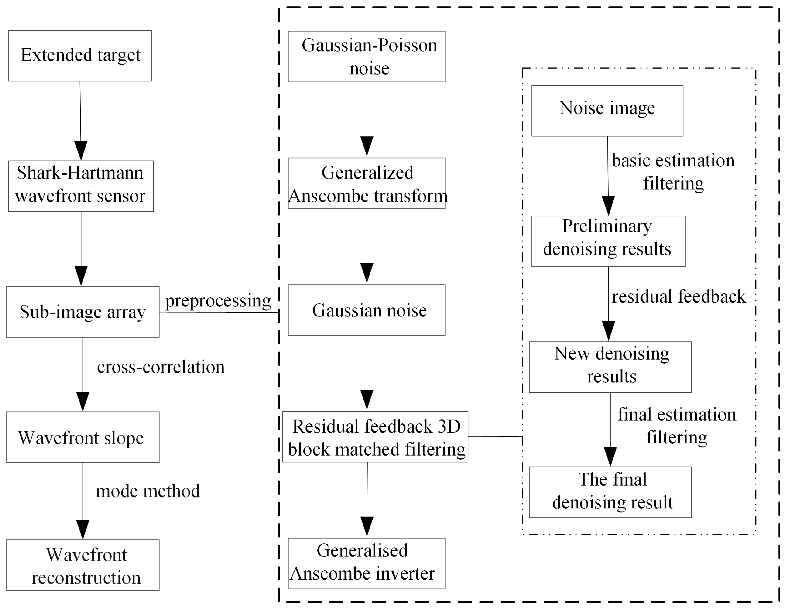
2.2. The Extended Target Image Preprocessing Method with a Low Signal-to-Noise Ratio

Extended target Shack–Hartmann wavefront sensors introduce a series of noises that adversely affect the detection accuracy. Thus, preprocessing of the sub-image array is necessary to enhance the accuracy of detection. The flowchart of the method proposed in this paper is illustrated in Figure 1.

2.3. Generalized Anscombe Transform

In the extended target Shack–Hartmann wavefront sensor for measurement, the transmitted signal is affected and interfered with by a variety of factors, including environmental stray light, device characteristics, detector characteristics, and other factors, which introduces a variety of noise. According to statistical law, its noise distribution includes two types: signal-independent Gaussian noise and signal-dependent Poisson noise [29,30,31]. The noise model equation is represented by Equation (9):

$$s\left(x\right)=a·p\left(s_0\left(x\right)\right)+n\left(x\right),$$

(9)

where $s\left(x\right)$ is a noisy image, $s_0\left(x\right)$ is a clear image, x denotes any pixel point, a is the gain, n is Gaussian noise with mean m and standard deviation $\sigma$, and $p$ is the Poisson noise.

The mutual correlation method is commonly employed to mitigate the impact of noise signals in the sub-image array on the relative error of offsets. However, this method overlooks the characteristics of the image noise. Therefore, this paper employs a method to enhance the signal-to-noise ratio. Conventional image noise processing algorithms typically assume the noise to be Gaussian white noise, while in practical detection, the detector generates Gaussian–Poisson noise. To tackle this issue, the detection noise is initially transformed into Gaussian noise. Subsequently, an algorithm is applied to effectively eliminate the Gaussian noise, thereby reducing computational complexity and saving processing time. This conversion process is known as the variance stabilizing transformation (VST), where the generalized Anscombe transform is frequently employed as a nonlinear transformation in image processing.

According to Equation (9), each pixel value $x_1$ observed can be expressed as:

$$x_1=a·p\left(y_1\right)+n,$$

(10)

where $n\left(m,{\sigma }_1^2\right)$, the Poisson distribution p parameter is ${\lambda }_0$, a is the gain, and $y_1$ is the pixel point of the clear image corresponding to the acquisition of pixel $x_1$. At this point, the variance is $Var\left(x_1\right)={\sigma }^2+a^2{\lambda }_0$, and the process of the generalized Anscombe transform is shown in Equation (11) below:

$$f\left(x_1\right)=\left\{\begin{array}{c}\hfill \frac{2}{a}\sqrt{a{x}_1+\frac{3}{8}{a}^2+{{\sigma }_1}^2-am},x_1>-\frac{3}{8}a-\frac{{{\sigma }_1}^2}{a}+m\\ \hfill 0,x_1\le -\frac{3}{8}a-\frac{{{\sigma }_1}^2}{a}+m\end{array}\right..$$

(11)

The transformed variance $Var\left(f\left(x_1\right)\right)=a/4$, and there is only Gaussian noise in the subaperture image.

2.4. Generalized Anscombe transform

After completing the above transformations, for Gaussian white noise, 3D block-matched filtering with residual feedback is introduced for noise reduction, and the above-improved method is referred to as the GFBM3D algorithm.

The BM3D consists of two stages, basic estimation filtering and final estimation filtering [32,33,34,35], which utilize the similarity between image blocks for noise reduction. The basic estimation stage consists of block matching grouping, 3D collaborative hard threshold filtering, and aggregated weighted filtering. The final estimation stage consists of block matching grouping, 3D collaborative Wiener filtering, and aggregated weighted filtering.

The noise reduction results are further improved by residual feedback because the residual feedback can rejoin the high-frequency signals that have not been processed by the BM3D algorithm into the input image, which makes the BM3D algorithm better able to process these high-frequency signals. The specific implementation method is as follows: take the difference between the noisy image and the initial denoising result to obtain a residual image. Add the residual image to the initial denoising result to obtain a new input image and proceed with further denoising.

2.5. Generalized Anscombe Inverter

After processing the signal matrix using the above noise reduction method, the inverse transformation is performed to obtain the actual noise-reduced sub-image array. The expression for the inverse transformation is shown in Equation (12):

$$f_{\sigma }{\left(y\right)}^{-1}=\frac{1}{4}{y}^2+\frac{1}{4}\sqrt{\frac{3}{2}{y}^{-1}}-\frac{11}{8}{y}^{-2}+\frac{5}{8}\sqrt{\frac{3}{2}{y}^{-3}}-\frac{1}{8}-{\sigma }^2.$$

(12)

3. Results

3.1. Simulation-Related Parameters

The detection system based on the extended target Shack–Hartmann wavefront sensor is mainly composed of a telescope and a Shack–Hartmann wavefront detector. To study the effect of the signal-to-noise ratio of the subaperture image on the offset detection accuracy, a sunspot image is selected as a reference for analysis on the Hinode website, and the sunspot image is shown in Figure 2. The main parameters are operating wavelength 1.064 $\mathsf{\mu }$m, Shack–Hartmann aperture: 0.07 m, and total number of subapertures 4 × 4; after screening the subapertures with better imaging effect, the number of effective subapertures is 12, the number of pixels corresponding to each subaperture is 256 × 256, and the focal length is 0.25 m. The subaperture image consists of the sunspot image and the system’s point spread function (PSF). Function (PSF) is convolved to form the extended target sub-image array as shown in Figure 3.

Based on the theoretical analysis and the system model, the relevant simulation is carried out, and the main steps are: 1. The second-order Zernike is used to simulate the offset of the subaperture images, and Gauss–Poisson noise is added to the offset sub-image array; 2. We obtain the extended target-related Shack–Hartmann sub-image array at a low signal-to-noise ratio and then preprocess the sub-image array; 3. We calculate the relevant Shack–Hartmann subaperture image offsets using the normalized intercorrelation method, obtain the wavefront slope, and solve for the mode coefficients, to reconstruct the wavefront.

To verify the effectiveness of the algorithm, comparison experiments are carried out in terms of the noise reduction effect, the relative error of the offset calculation, and the wavefront reconstruction coefficients, respectively.

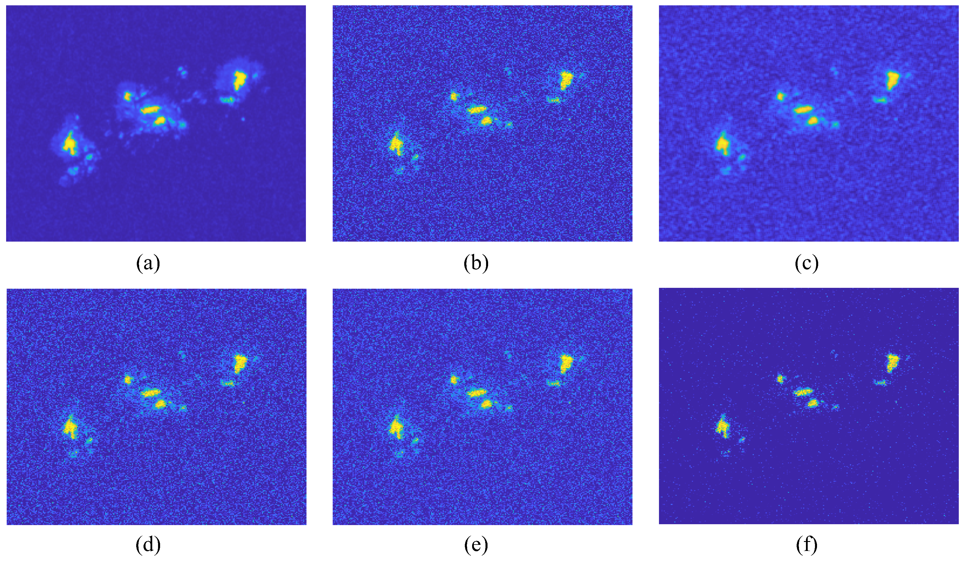
3.2. Subaperture Image Noise Reduction Simulation

The noise model is the Gaussian–Poisson noise model, which is firstly generalized Anscombe transformed to convert the Gaussian–Poisson noise to Gaussian noise; secondly, residual feedback is performed on the 3D block matched filtering. Thus, noise reduction is performed on Gaussian noise, and finally, inverse transformation is performed to bring it back to the initial domain.

The peak signal-to-noise ratio (PSNR) of the image is used to describe the noise level, which is calculated as follows:

$$PSNR=10{log}_{10}\left(\frac{max{\left(d\right(j\left)\right)}^2}{{\displaystyle \sum _{j=1}^N}{\left(d\left(j\right)-d_{\mathrm{noisy}}\left(j\right)\right)}^2/N}\right),$$

(13)

where $d\left(j\right)$ denotes the original image, $d_{noisy}\left(j\right)$ is the noisy image, and N is the total number of pixels in the image.

Figure 4 shows the noisy image under the noise model given in Equation (9), as well as the comparison images of individual subapertures after applying the mean filter, Gaussian filter, BM3D, and the denoising algorithm proposed in this paper (GFBM3D). The Gaussian noise has a mean value of $m=0$ and a standard deviation of $\sigma$ = 0.02, while the Poisson noise has a gain of $a=0.003$. From the figure, it can be seen that the use of the GFBM3D algorithm is closer to a clear image than the use of the three noise reduction algorithms mentioned above; at this time, the PSNR of the band noise image is 27 dB, and after the application of the GFBM3D algorithm, the PSNR is 33 dB, which makes the subaperture image effectively preprocessed.

3.3. Subaperture Offset Detection Simulation

In order to study the effect of the subaperture image noise on the correlation algorithm, the normalized cross-correlation algorithm is used to calculate the offset of the aberration image with respect to the reference image before and after the noise reduction and to obtain the corresponding offset calculation error, where the offset calculation error = (calculated offset − actual offset)/actual offset. The average offset calculation error is shown in

Table 1. Average offset calculation error after noise reduction by different methods.

Method	Average Offset Calculation Error
Noisy image	7.78
Mean filtering	5.4865
Gaussian filtering	7.7843
BM3D	7.60
GFBM3D	3.76

. From Table 1, it can be seen that the noise reduction algorithm with Gaussian filtering is less effective compared to the noisy image, and the error is not reduced; after applying the mean filtering and BM3D algorithm for noise reduction, the error is improved by about 29.5% and 2.35%. The generalized Anscombe transform is introduced, residual feedback is added before the BM3D noise reduction, and the computational error of the offset is improved by 51.69%. The experiments show that the application of the algorithm in this paper better enables the accuracy improvement of the extended target Shack–Hartmann wavefront detection to be guaranteed.

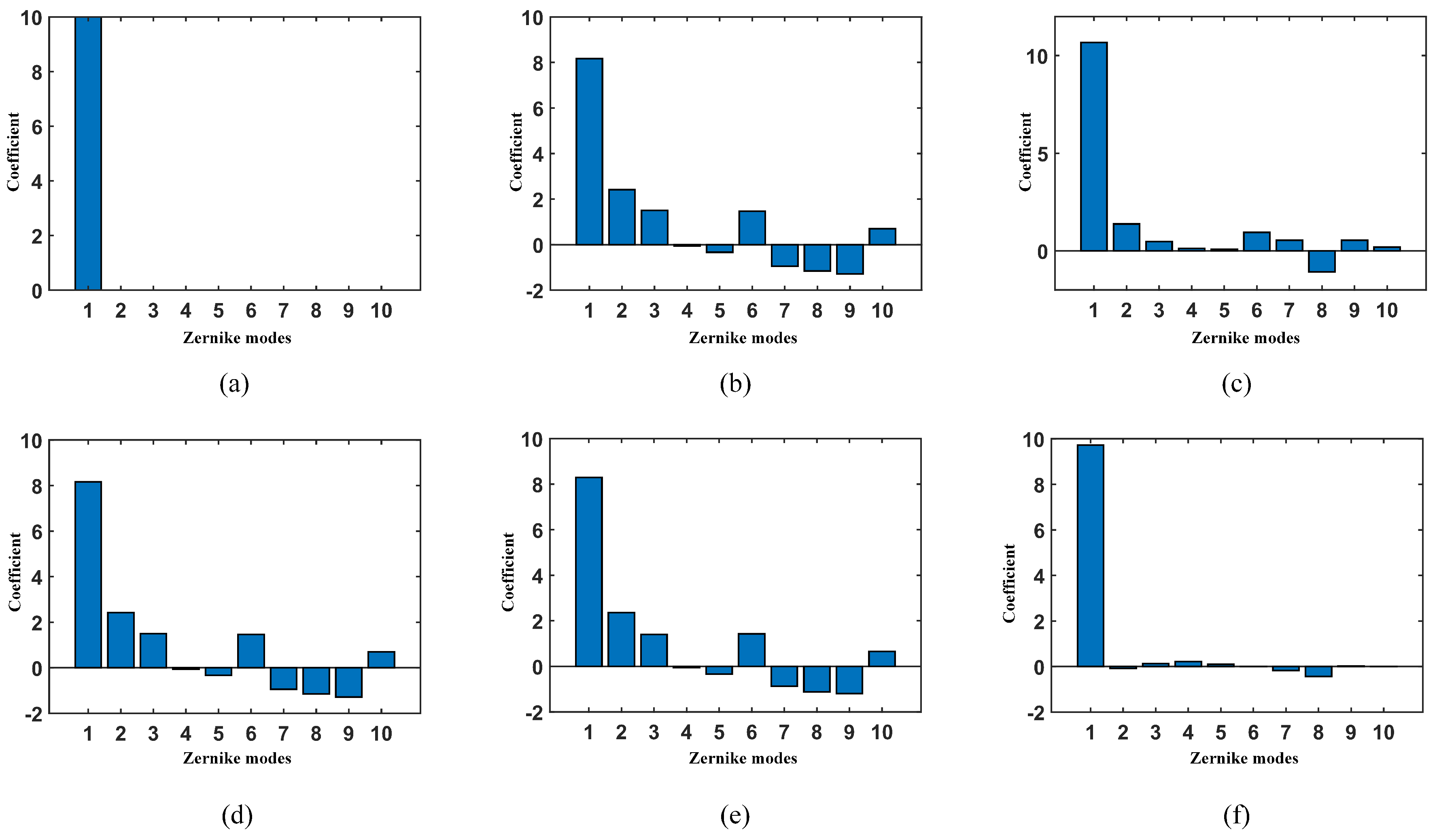
3.4. Simulation and Analysis of the Wavefront Reconstruction

In the Shack–Hartmann wavefront detector, in order to further verify the effectiveness of the noise reduction algorithm in this paper, the wavefront reconstruction is carried out using the mode method and evaluated with the root mean square error. The reconstructed Zernike coefficients are shown in Figure 5, corresponding to the second term of the Zernike polynomial with a coefficient of 10. Figure 5b–f show the distorted reconstructed wavefront Zernike coefficients corresponding to the subaperture images subjected to noise interference, those after the noise reduction is carried out, and the comparisons with Figure 5a, respectively, indicate that the reconstructed wavefront after noise reduction is closer to the added value. The coefficients are closer to the added values, while the noise reduction using the GFBM3D algorithm is closest to the added values. The root mean square errors are shown in

Table 2. RMSE of reconstruction coefficients after noise reduction by different methods.

Method	Root Mean Square Error
Noisy image	1.3440
Mean filtering	0.7251
Gaussian filtering	1.3440
BM3D	1.2827
GFBM3D	0.1941

below.

As can be seen from Table 2, the effect of the noise reduction algorithm using Gaussian filtering is still poor, and the root mean square error after applying the mean filtering and BM3D algorithm for noise reduction is improved by 46.05% and 4.56%, respectively; whereas, after applying the GFBM3D algorithm for noise reduction, it is improved by 85.56%, and the reconstruction results further indicate that the algorithm of this paper for the preprocessing of subaperture images can effectively improve the Shack–Hartmann wavefront detector’s wavefront detection accuracy.

4. Conclusions

Aiming at the problem of noise affecting the extended target Shack–Hartmann wavefront detection accuracy enhancement, this paper proposes an image preprocessing method before the calculation of the subaperture image offset. Gaussian–Poisson noise is converted to Gaussian noise by the generalized Anscombe transform, residual feedback is performed on the 3D block matched filtering for the noise reduction of the sub-image arrays, and offset computation is performed by the normalized mutual correlation algorithm; hence, wavefront reconstruction and a detailed simulation study was carried out to compare it with three commonly used noise reduction methods. The results show that the proposed method reduces the relative error of the subaperture offset calculation by 51.69%, improves the Zernike coefficient of the corresponding aberration reconstruction wavefront by 85.56%, improves the detection accuracy based on effectively retaining the image details, and does not need to adjust the algorithm parameters dynamically, which makes it more practical and adaptable in the application of practical systems.

References

1. Hu, J.; Chen, T.; Lin, X.; Wang, L.; An, Q.; Wang, Z. Improved wavefront reconstruction and correction strategy for adaptive optics system with a plenoptic Sensor. IEEE Photonics J. 2021, 13, 6801008. [Google Scholar] [CrossRef]
2. Primot, J. Theoretical description of Shack–Hartmann wave-front sensor. Opt. Commun. 2003, 222, 81–92. [Google Scholar] [CrossRef]
3. Shahidi, M.; Yang, Y. Measurements of ocular aberrations and light scatter in healthy subjects. Optom. Vis. Sci. 2004, 81, 853–857. [Google Scholar] [CrossRef] [PubMed]
4. Perez, G.M.; Manzanera, S.; Artal, P. Impact of scattering and spherical aberration in contrast sensitivity. J. Vis. 2009, 9, 19. [Google Scholar] [CrossRef]
5. Leith, E.N.; Hoover, B.G.; Dilworth, D.S.; Naulleau, P.P. Ensemble-averaged Shack–Hartmann wave-front sensing for imaging through turbid media. Appl. Opt. 1998, 37, 3643–3650. [Google Scholar] [CrossRef]
6. Galaktionov, I.; Sheldakova, J.; Nikitin, A.; Toporovsky, V.; Kudryashov, A. A Hybrid Model for Analysis of Laser Beam Distortions Using Monte Carlo and Shack–Hartmann Techniques: Numerical Study and Experimental Results. Algorithms 2023, 16, 337. [Google Scholar] [CrossRef]
7. Tao, X.; Dean, Z.; Chien, C.; Azucena, O.; Bodington, D.; Kubby, J. Shack-Hartmann wavefront sensing using interferometric focusing of light onto guide-stars. Opt. Express 2013, 21, 31282–31292. [Google Scholar] [CrossRef]
8. Li, X.; Li, X.; Wang, C. Optimum threshold selection method of centroid computation for Gaussian spot. In AOPC 2015: Image Processing and Analysis; SPIE: Bellingham, WA, USA, 2015; Volume 9675, p. 967517. [Google Scholar]
9. Vargas, J.; Restrepo, R.; Belenguer, T. Shack-Hartmann spot dislocation map determination using an optical flow method. Opt. Express 2014, 22, 1319–1329. [Google Scholar] [CrossRef]
10. Vargas, J.; Restrepo, R.; Estrada, J.; Sorzano, C.; Du, Y.Z.; Carazo, J. Shack–Hartmann centroid detection using the spiral phase transform. Appl. Opt. 2012, 51, 7362–7367. [Google Scholar] [CrossRef]
11. Wei, P.; Li, X.; Luo, X.; Li, J. Analysis of the wavefront reconstruction error of the spot location algorithms for the Shack–Hartmann wavefront sensor. Opt. Eng. 2020, 59, 043103. [Google Scholar] [CrossRef]
12. Shen, T.T.; Zhu, L.; Kong, L.; Zhang, L.Q.; Rao, C.H. Real-time Image Shift Detection with Cross Correlation Coefficient Algorithm for correlating Shack-Hartmann Wavefront Sensors Based on FPGA and DSP. Appl. Mech. Mater. 2015, 742, 303–311. [Google Scholar] [CrossRef]
13. Xia, M.; Li, C.; Liu, Z. Adaptive threshold selection method for Shack-Hartmann wavefront sensors. Opt Precis. Eng 2010, 18, 334–340. [Google Scholar]
14. Yang, W.; Wang, J.; Wang, B. A method used to improve the dynamic range of Shack–Hartmann wavefront sensor in presence of large aberration. Sensors 2022, 22, 7120. [Google Scholar] [CrossRef] [PubMed]
15. Wang, Y.; Chen, X.; Cao, Z.; Zhang, X.; Liu, C.; Mu, Q. Gradient cross-correlation algorithm for scene-based Shack-Hartmann wavefront sensing. Opt. Express 2018, 26, 17549–17562. [Google Scholar] [CrossRef] [PubMed]
16. Poyneer, L.A. Scene-based Shack-Hartmann wave-front sensing: Analysis and simulation. Appl. Opt. 2003, 42, 5807–5815. [Google Scholar] [CrossRef] [PubMed]
17. Rimmele, T.R.; Marino, J. Solar adaptive optics. Living Rev. Sol. Phys. 2011, 8, 2. [Google Scholar] [CrossRef]
18. Jiang, P.; Zhao, M.; Zhao, W.; Wang, S.; Yang, P. Image enhancement of Shack-Hartmann wavefront sensor with non-uniform illumination. In Proceedings of the 10th International Symposium on Advanced Optical Manufacturing and Testing Technologies: Advanced Optical Manufacturing and Metrology Technologies; SPIE: Bellingham, WA, USA, 2021; Volume 12071, p. 120710P. [Google Scholar]
19. Li, X.; Li, X. Improvement of correlation-based centroiding methods for point source Shack–Hartmann wavefront sensor. Opt. Commun. 2018, 411, 187–194. [Google Scholar] [CrossRef]
20. Mao, H.; Liang, Y.; Liu, J.; Huang, Z. A noise error estimation method for Shack-Hartmann wavefront sensor. In AOPC 2015: Telescope and Space Optical Instrumentation; SPIE: Bellingham, WA, USA, 2015; Volume 9678, p. 967811. [Google Scholar]
21. Kong, F.; Polo, M.C.; Lambert, A. Centroid estimation for a Shack–Hartmann wavefront sensor based on stream processing. Appl. Opt. 2017, 56, 6466–6475. [Google Scholar] [CrossRef]
22. Anugu, N.; Garcia, P.J.; Correia, C.M. Peak-locking centroid bias in shack–hartmann wavefront sensing. Mon. Not. R. Astron. Soc. 2018, 476, 300–306. [Google Scholar] [CrossRef]
23. Zhao, P.; Wang, X.; Yang, F.; Min, Z. Extremely Weak Signal Detection Algorithm of Multi-Pixel Photon Detector. J. Phys. Conf. Ser. 2023, 2476, 012026. [Google Scholar] [CrossRef]
24. Zhou, H.; Zhang, L.; Zhu, L.; Bao, H.; Guo, Y.; Rao, X.; Zhong, L.; Rao, C. Comparison of correlation algorithms with correlating Shack-Hartmann wave-front images. In Proceedings of the Society of Photo-Optical Instrumentation Engineers (SPIE) Conference Series; SPIE: Bellingham, WA, USA, 2016; Volume 10026, p. 100261B. [Google Scholar]
25. Wang, G.; Hou, Z.; Qin, L.; Jing, X.; Wu, Y. Simulation Analysis of a Wavefront Reconstruction of a Large Aperture Laser Beam. Sensors 2023, 23, 623. [Google Scholar] [CrossRef] [PubMed]
26. Fried, D.L. Least-square fitting a wave-front distortion estimate to an array of phase-difference measurements. JOSA 1977, 67, 370–375. [Google Scholar] [CrossRef]
27. Löfdahl, M.G. Evaluation of image-shift measurement algorithms for solar Shack-Hartmann wavefront sensors. Astron. Astrophys. 2010, 524, A90. [Google Scholar] [CrossRef]
28. Rimmele, T.R.; Radick, R.R. Solar adaptive optics at the National Solar Observatory. Adapt. Opt. Syst. Technol. 1998, 3353, 72–81. [Google Scholar]
29. Xie, M.; Zhang, Z.; Zheng, W.; Li, Y.; Cao, K. Multi-Frame Star Image Denoising Algorithm Based on Deep Reinforcement Learning and Mixed Poisson–Gaussian Likelihood. Sensors 2020, 20, 5983. [Google Scholar] [CrossRef] [PubMed]
30. Zou, C.; Xia, Y. Bayesian dictionary learning for hyperspectral image super resolution in mixed Poisson–Gaussian noise. Signal Process. Image Commun. 2018, 60, 29–41. [Google Scholar] [CrossRef]
31. Chouzenoux, E.; Jezierska, A.; Pesquet, J.C.; Talbot, H. A convex approach for image restoration with exact Poisson–Gaussian likelihood. SIAM J. Imaging Sci. 2015, 8, 2662–2682. [Google Scholar] [CrossRef]
32. Astari, F.M.; Mulyantoro, D.K.; Indrati, R. Analysis of BM3D Denoising Techniques to Improvement of Thoracal MRI Image Quality; Study on Low Field MRI. J. Med. Imaging Radiat. Sci. 2022, 53, S24. [Google Scholar] [CrossRef]
33. Ri, G.I.; Kim, S.J.; Kim, M.S. Improved BM3D method with modified block-matching and multi-scaled images. Multimed. Tools Appl. 2022, 81, 12661–12679. [Google Scholar] [CrossRef]
34. Li, Y.; Zhang, J.; Wang, M. Improved BM3D denoising method. IET Image Process. 2017, 11, 1197–1204. [Google Scholar] [CrossRef]
35. Feruglio, P.F.; Vinegoni, C.; Gros, J.; Sbarbati, A.; Weissleder, R. Block matching 3D random noise filtering for absorption optical projection tomography. Phys. Med. Biol. 2010, 55, 5401. [Google Scholar] [CrossRef] [PubMed]
Figure 1. Flowchart of the method.
Applsci 13 10004 g001
Figure 2. Image of sunspot.
Applsci 13 10004 g002
Figure 3. Expansion of the target sub-image array.
Applsci 13 10004 g003
Figure 4. Comparison of the subaperture images after noise reduction by different methods. (a) Original image. (b) Noisy image. (c) Mean filtering. (d) Gaussian filtering. (e) BM3D (f) GFBM3D.
Applsci 13 10004 g004
Figure 5. The pattern method reconstructs the wavefront Zernike coefficients. (a) The added distortion wave surface. (b) Noisy image. (c) Mean filtering. (d) Gaussian filtering. (e) BM3D. (f) GFBM3D.
Applsci 13 10004 g005