A Novel Way of Optimizing Headlight Distributions Based on Real-Life Traffic and Eye-Tracking Data Part 2: Analysis of Real-World Traffic Environments Data in Germany

Abstract

In order to find optimized headlight distributions based on real traffic data, a three-step approach has been chosen. Since the complete investigations are too extensive to fit into one single publication, this paper is the second of three papers. Over the course of these papers, a novel way to optimize automotive light distributions based on real-life traffic and eye-tracking data is presented. Over all three papers, 119 test subjects participated in the studies, with over 15,000 km of driving, including recordings of gaze behavior, light data, detection distances and other objects in traffic. In the first paper, an ideal headlight distribution for straight roads with no other road users was identified. The second paper aims to collect the data required to modify this idealized headlight distribution for use on real roads. The first step is to find the extent to which real roads differ from an ideal, straight road. To do this, the German traffic space was analyzed. A new test vehicle recorded video and GPS data over a selected route. The video data were then evaluated by a machine learning algorithm. Object recognition software was used to find different traffic participants and road signs. Camera calibrations were used to find the exact angles of these objects. Using publicly available road data combined with the recorded GPS data, the video data were split into different road categories, and traffic object distributions were calculated for urban roads, country roads and motorways. The resulting analyses provided representative distributions of vehicles and highway signs along different types of roadways and roadway geometries. The GPS data were also used to find the curvature distributions along the selected route. These data were then used to optimize segment sizes for an adaptive driving beam. Overall, increasing the number of segments above 100 did not have appreciable benefits. These data will also be used in the third paper, where along the same route, the gaze distribution of drivers was recorded and analyzed.

1. Introduction

While the first paper of this series of three papers focused on the required intensity and an idealized light distribution for modern headlamps, this second paper now focuses on roads in real-world traffic. While there have been previous publications on traffic and traffic distributions [1,2,3,4] and on average road design in Europe, a lot has changed over the last several years. With more and more vehicles on the road every year [5], combined with new technologies both in road lighting (light emitting diode (LED) lights) and in vehicle lighting, and considering rapid recent advances in computing power and computer vision, new data need to be acquired to confirm the characteristics of roads at the present time.

The new data are then used to optimize the idealized light distribution from the first paper, based on real traffic data. The overall idea is that the current headlight distributions that are covered by the UN ECE Regulation R123 for county roads (class C), urban roads (class V), motorways (class E) and driving under adverse weather conditions (class W) [6] are not the optimal solutions. This is due in large part to technological limitations whereby differences among these classes are mostly achieved by swiveling and dimming the standard passing beam, the primary solutions available when these classes were defined. Further, the roadway geometries were somewhat idealized and abstract, because until recently, it was not possible to collect comprehensive data on the locations of roadway edges, traffic signs, or other vehicles along the road over a large set of roadway environments. The use of video capture and artificial intelligence algorithms for recording and classifying such information has only become available recently. It should be noted that this does not necessarily imply that the current headlight distributions are not functional. The new analytical methods could provide reassurance that existing headlight beam patterns are in fact appropriately designed, or they might provide insight into improvements. Either outcome would be beneficial situation for nighttime driving safety.

While the detailed process for proposing an optimized light distribution by this paper series will be explained in the third and final paper, the short summary is that light is needed wherever critical objects are located within the traffic space [7]. As Huhn shows, even for oncoming traffic at night it is beneficial for the human eye to add light into the direct surroundings of those vehicles to minimize glare effects and help with short-term adaptation in the presence of light sources from oncoming traffic. Numerous investigations of visibility requirements from advanced headlighting systems and illumination needs for visually guided behavior have been undertaken by Müller, Rosenhahn, Kanna, Erkan, Reagan, Funk, Waldner, Cengiz and Winter [8,9,10,11,12,13,14,15,16,17,18].

When looking at different situations, it becomes obvious that a traffic space analysis from the driver’s view should be split into at least three different sections: urban roads, country roads and motorways. Driving in urban environments will lead to completely different lighting situations due to the presence of fixed road lighting, advertisements and much denser traffic. Erkan has proposed a dynamic lighting function that limits the light output on urban roads based on a constant luminance level. Since the main light in urban environments comes from fixed road lighting, additional lighting from the car’s headlamps can be limited [19].

Country roads could be regarded as the standard road for headlight distributions. They have relatively simple road layouts, with mostly one lane in each direction. Fixed road lighting is rare, there is reduced traffic density, driving speeds are often limited to (on average) 80 $\mathrm{k}\mathrm{m} {\mathrm{h}}^{-1}$, and as shown by Kuhl, there is a nearly normal distribution for the road curvature [4].

Motorways on the other hand can be rather complicated, with at least two lanes but sometimes four or more lanes in each direction. There can also be vastly different driven speeds, between 60 $\mathrm{k}\mathrm{m} {\mathrm{h}}^{-1}$ and even unlimited speeds on some motorways in Germany. Depending on which lane a vehicle is in, the requirements for the headlight distribution will change due to the speed, the position of other vehicles when they are passing or are being passed and the possible relative speeds between vehicles. Furthermore, traffic signs are often located at different positions compared to urban and country roads. One possibly simplifying factor is that no pedestrians and cyclists are allowed on motorways.

However, as already indicated by the different situations that may occur on motorways, the same differentiation is also easily possible for urban roads with different intersections, different ambient lighting situations, different traffic scenarios and more. The optimum for the driver would be an unlimited number of light distributions that could easily and seamlessly be produced by the headlight at the appropriate time. These papers therefore propose a novel approach to achieving these light distributions.

Additionally, the data acquired here are used to optimize the size of individual LED segments for adaptive driving beam (ADB) headlamps. Such a method was proposed by Moisel, Totzauer and some authors of this paper [20,21,22]. However, the proposal of Moisel was based on a logical analysis and was not backed-up by empirical data. The proposal shown by Totzauer, which was based on a simulation, seemed to result in illogical distributions in some cases. The proposal presented previously by the authors of this paper seemed to yield appropriate outcomes but was only based on simulation data as well. Thus, one of the overall objectives is to validate those simulations with real traffic data and identify differences that were not covered by the simulation data. In this investigation, it was of course necessary to select a finite roadway environment along which to record geometric and traffic conditions. As is described below, it is hoped that this environment is representative of roads in Europe, or at least in Germany. It must be recognized that the success of the headlight beam distributions to be derived from this analysis will depend on the extent to which the test course we selected is indeed representative of real-world general conditions. Nonetheless, even if the roads used to generate the traffic environment data were not representative, the analytical approach outlined here could be applied to a larger, more representative dataset.

Investigations

In the following sections, the two main studies are presented. Each section starts by describing the test setup, the test method, the test subjects and then the results.

We refrain from first describing the methodology for all the performed investigations and then discussing the results, in order to preserve a logical consistency within each investigation.

2. German Traffic Space Analysis

As mentioned previously, the overall traffic space has changed drastically in recent decades with about 10% more vehicles on our roads since 2015 and very different lighting situations due to the changes in road and vehicle lighting (e.g., the transition from halogen and sodium to LED lighting).

As no single description of the traffic space from recent years exists that includes all the required data to classify the space, and since the goal of these papers is to connect this road analysis data with gaze behavior, the traffic space analysis was done completely from scratch. The method and equipment used are explained briefly in the following sections, followed by the resulting traffic distributions.

2.1. Test Vehicle

A BMW 3 Series passenger car with LED headlights and high beam assist function from the TU Darmstadt was used. The vehicle has a head-up display and satellite navigation. The driving for this activity was performed by test subjects, and for the third paper in this series, their gaze behavior was recorded as well along the driven route, as previously programmed into the navigation system. The 54 test subjects were all aged between 19 and 40 years of age, had a valid driver’s license and were given time on the university’s parking space to get used to the vehicle.

The setup for the eye-tracking study, the test subjects and the car’s settings will be explained in detail in the third paper of the series, where these details are relevant. Because the data collection in this phase was made using a passenger car, the resulting geometric distributions of other vehicles and signs may not accurately reflect the same locations at which these features would be seen from other vehicle types, such as sport-utility vehicles or heavy trucks.

2.1.1. Test Equipment

To evaluate the traffic space, an individual stereo camera setup was constructed, based on two GigE uEye cameras with a pixel resolution of 2056 by 1542 each, with an 8 $\mathrm{m}$$\mathrm{m}$ Fuji-film lens. This provides a field of view of ±20${}^{°}$ horizontally and ±6${}^{°}$ vertically, thereby covering the important part for headlight distributions. This setup was hard-mounted behind the rear view mirror to minimize its influence on the driver as much as possible. With this camera setup, it was possible to select all relevant parameters such as frame rate (set to 25 frames per second), exposure and ISO level to be controlled by the self-programmed GUI from the rear seat. The aperture was controlled manually and set to a fixed value. The program also logged the time stamp for each individual frame, logged when frames were missing and logged the exposure for every frame as well. Additionally, a GPS system recorded the position, speed and angular direction for each frame as well. While most of these values were not utilized in this paper, the data are available for further investigations by the TU Darmstadt.

2.1.2. Object Recognition

The data were recorded locally in the vehicle and sent for offline evaluation to the TU Darmstadt’s server at a later time. Here, object recognition software was used to identify the following objects:

• Pedestrians;
• Cars;
• Buses;
• Trucks;
• Cyclists;
• Bicycles;
• Traffic signs.

As a baseline, the software was trained with the Cityscapes Dataset [23]. To train the software on the recorded dataset, an additional training with 250 hand-labeled images recorded during these nighttime drives was used. The detailed process is not explained here but can be found in [24,25,26,27,28].

The evaluation of the data showed that the object recognition performance led to around 70% confidence when identifying vehicles, which was the most important class for this paper. All other classes had a lower confidence performance, and especially for pedestrians, which were rather rare in our recordings, only a confidence of 40% was achieved. However, training the data with more images from our recordings did not lead to any improvements and Pkulzc showed that these results were to be expected [29].

2.2. Route

Since the goal of this paper series was to combine object and gaze data, a single route was chosen, that was driven a total of 108 times: 54 times during the day and 54 times during the night. The day drives were conducted to compare the gaze behavior during day and night but are not relevant for this study; therefore, this paper only focuses on the 54 nighttime drives.

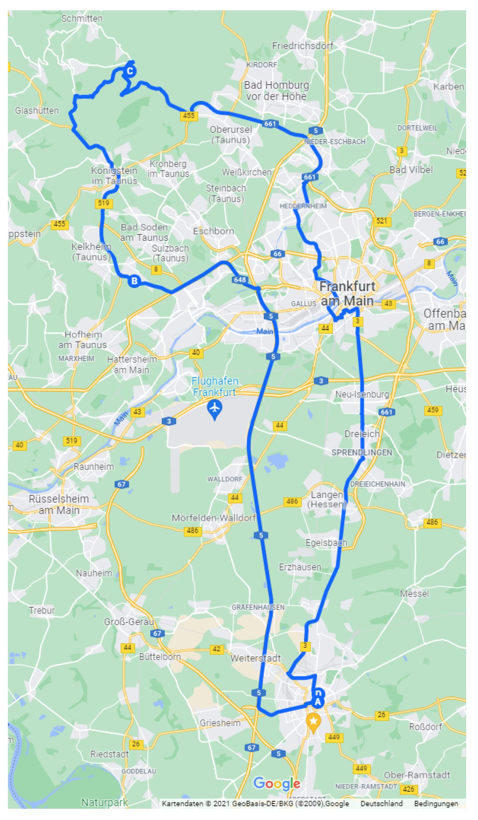
The route was selected to start in Darmstadt at the university. From there, the first section went straight onto a motorway. This was done, so that the test subjects (drivers) would be able to accommodate to the vehicle before heading into more stressful urban roads.

After the motorway section, the route entered the Taunus, a small mountain range near Frankfurt with many narrow bends up and down the mountains. From there, the country roads were taken directly into the city center of Frankfurt am Main. The last section was from Frankfurt back to the University of Darmstadt along nearly straight country roads. The complete route is shown in Figure 1.

Overall, this route was chosen to contain, depending on traffic and time of day, similar numbers of country roads and motorways, while collecting the most data in urban environments since this was expected to be the most complex road type. Overall, around 49% of the driving time was spent in the urban areas and 29% on country roads, with the rest (22%) being on motorways.

How these data were classified is explained in the next section.

2.2.1. Classification

In order to classify the data as one of the three main classes, the Open Street Maps Database (OSM) was used. The OSM Database consists of nodes connected by ways. Each node contains information based on their GPS position. The information contains, for example, highway type, references to street names such as the A5 (Motorway 5), the known (permanent) speed limit, the number of lanes, the city this node belongs to and more. The most important pieces of information for this study were the different highway types that were included in the chosen route [30]:

• Motorway: A restricted-access major divided motorway, normally with two or more running lanes plus an emergency hard shoulder. Equivalent to the freeway, Autobahn, etc.
• Motorway link: the link roads (slip roads/ramps) leading to/from a motorway from/to a motorway or lower-class motorways, normally with the same motorway restrictions.
• Trunk: The most important roads in a country’s system that are not motorways. (Need not necessarily be divided motorways.)
• Trunk link: the link roads (sliproads/ramps) leading to/from a trunk road from/to a trunk road or lower-class motorway.
• Primary: The next most important roads in a country’s system. (Often linking larger towns.)
• Primary link: the link roads (sliproads/ramps) leading to/from a primary road from/to a primary road or lower-class motorway.
• Secondary: The next most important roads in a country’s system. (Often linking towns.)
• Tertiary: The next most important roads in a country’s system. (Often linking smaller towns and villages)
• Unclassified: The least important through roads in a country’s system—i.e., minor roads of a lower classification than tertiary, but which serve a purpose other than access to properties. These often link villages and hamlets. (The word “unclassified” is a historical artefact of the UK road system and does not mean that the classification is unknown.)
• Residential: Roads which serve as access to housing, without the function of connecting settlements. Often lined with housing.
• Service: For access roads to or within an industrial estate, camp site, business park, car park etc. Can be used in conjunction with service = * to indicate the type of usage and with access = * to indicate who can use it and in what circumstances.
• Footway: For designated footpaths, i.e., mainly/exclusively for pedestrians. This includes walking tracks and gravel paths. If bicycles are allowed as well, this can be indicated by adding a bicycle = yes tag. Should not be used for paths where the primary or intended usage is unknown. Use motorway = pedestrian for pedestrianized roads in shopping or residential areas and motorway = track if it is usable by agricultural or similar vehicles.
• Path A nonspecific path. Use motorway = footway for paths mainly for pedestrians, motorway = bikeway for one also usable by cyclists, motorway = bridleway for ones available to horses as well as pedestrians and motorway = track for ones which are passable by agriculture or similar vehicles.

From these data, the three main road types (urban, country and motorways) were derived.

Rural Roads

• The motorway type is either footpath, path, residential or service.
• The motorway type is either primary, primary link secondary, tertiary or unclassified, and the speed limit is equal to or lower than 50 $\mathrm{k}\mathrm{m} {\mathrm{h}}^{-1}$.
• The motorway type is trunk or trunk link, and the speed limit is equal to or lower than 50 $\mathrm{k}\mathrm{m} {\mathrm{h}}^{-1}$ and the city is either Frankfurt or Darmstadt.

Country Roads

• The motorway type is either primary, primary link, secondary, tertiary or unclassified, the speed limit is higher than 50 $\mathrm{k}\mathrm{m} {\mathrm{h}}^{-1}$, and there are two or more lanes available.
• The motorway type is either primary, primary link, secondary, tertiary or unclassified while the speed limit is higher than 50 $\mathrm{k}\mathrm{m} {\mathrm{h}}^{-1}$ and below 100 $\mathrm{k}\mathrm{m} {\mathrm{h}}^{-1}$ with one available lane.

Motorways

• The motorway type is either motorway or motorway link and the speed limit is above 50 $\mathrm{k}\mathrm{m} {\mathrm{h}}^{-1}$.
• The motorway type is either trunk, trunk link, primary, primary link or secondary and a one way road, with more than one lane available.

All data points were checked for redundant or no categorization. Since the categorization rules oppose each other, no single GPS point was assigned two road types. A total of 552 GPS points could not be assigned to any of the three main categories. However, with a total of 83 million GPS points recorded, this was less than 0.1%. It needs to be mentioned here that only around 80% of the data points were assigned a motorway type by Open Street Maps, so 20% of all data were assigned a type only due to the other rules set in place.

Additionally, the road curvature was calculated. Since the proposed methods from Pratt and Ai [31,32] did not result in curves that fit to the collected data, the calculation was performed in a simple mathematical way.

In the first step, the GPS data were transformed into Universal Transverse Mercator (UTM) data. From this, the angle of the driven direction was calculated. The angle was then used to classify if a GPS point was part of a curve by calculating angular changes between two GPS points. If five successive points were deemed to be on a curve in a single direction, the curve radius was calculated by Equation (1)

$$\begin{array}{cc}\hfill 0& =x^2+y^2+2gx+fy+c\hfill \end{array}$$

(1a)

$$\begin{array}{cc}\hfill R& =\sqrt{g^2+f^2-c}\hfill \end{array}$$

(1b)

where the center point of the circle is located at $(-g,-f)$. This can be solved by a least square minimization as shown in Equation (2)

$$\begin{array}{cc}\hfill \left[\begin{array}{ccc}{x}_{i-5}& y_{i-5}& 1\\ x_{i-4}& y_{i-4}& 1\\ ⋮& ⋮& ⋮\\ x_i& y_i& 1\\ ⋮& ⋮& ⋮\\ x_{i+5}& y_{i+5}& 1\end{array}\right]\ast \overrightarrow{a}& =\left[\begin{array}{c}{x}_{i-5}^2+y_{i-5}^2\\ x_{i-4}^2+y_{i-4}^2\\ ⋮\\ x_i^2+y_i^2\\ ⋮\\ x_{i+5}^2+y_{i+5}^2\end{array}\right]\hfill \end{array}$$

(2)

$$\begin{array}{cc}\hfill g& =-0.5·a_1\hfill \\ \hfill f& =-0.5·a_2\hfill \\ \hfill R& =\sqrt{\frac{a_1^2+a_2^2}{4}-a_3}\hfill \end{array}$$

(3)

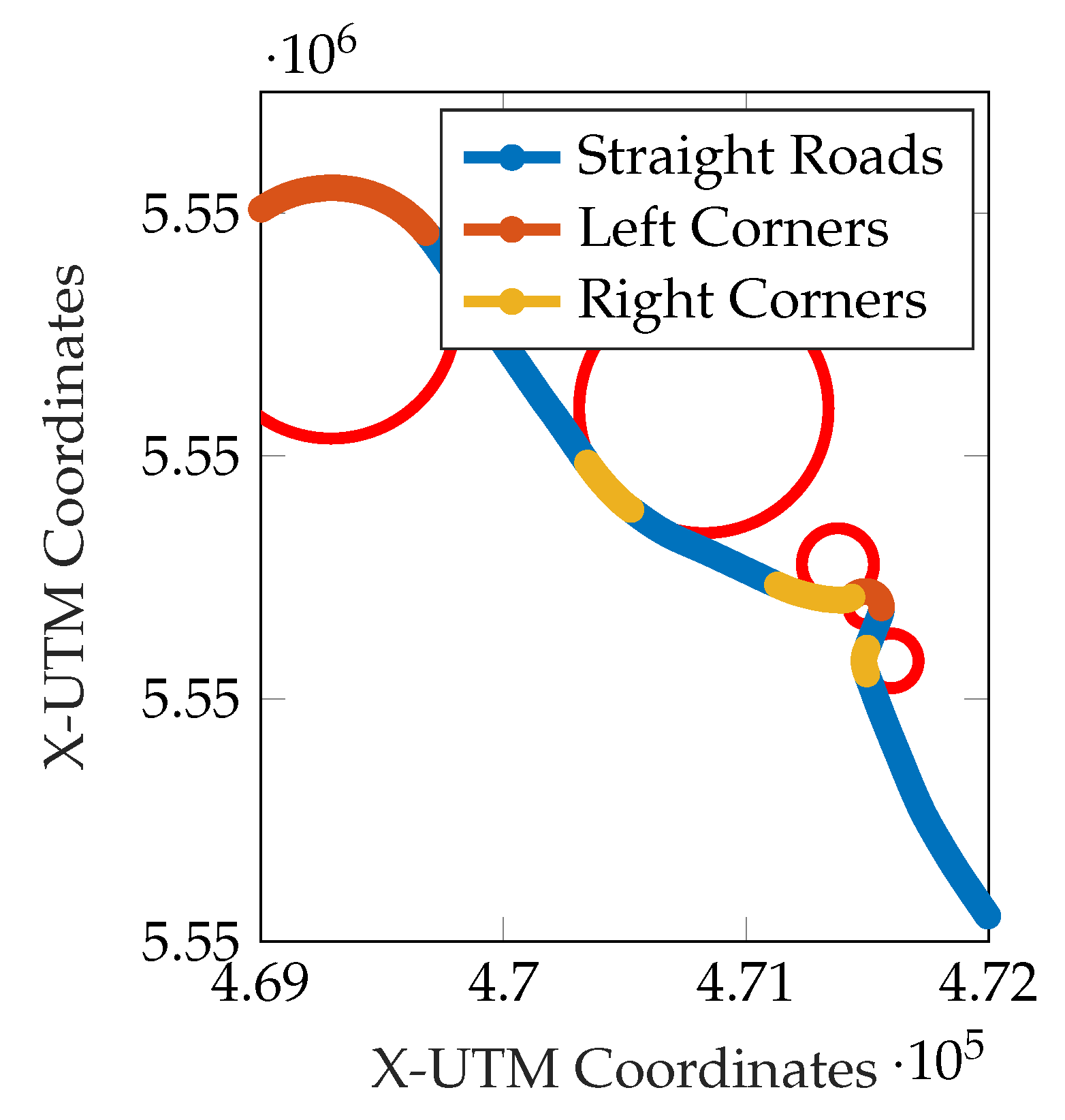
To exemplify the result of this calculation, a sample stretch of road with several identified curves, shown by their corresponding circles, is shown in Figure 2. The drive starts in the bottom right corner and moves to the top left corner, meaning that blue stretches of road mark straight roads, yellow stretches of road mark right curves, and orange roads mark left curves. The red circles mark the center $(-g,-f)$ of each curve and illustrate the calculated radius (R) of each corresponding curve.

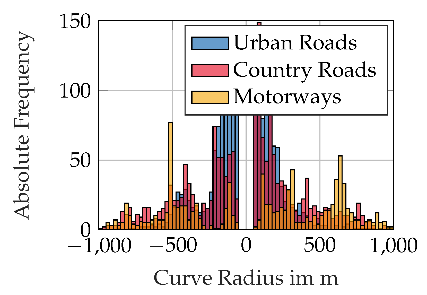
The curve radii found by this procedure, sorted by the three road categories, are presented in Figure 3.

As expected, motorways show the least number of narrow bends while urban roads show the most narrow bends of all three categories. The fact that left curves (negative radii) and right curves (positive radii) show the same overall number suggests that the route was well chosen in this regard. Thus, even if the roadway course used in this investigation is not exactly representative of all roadway environments throughout Germany, the symmetry of left/right curve distributions and the reasonable outcome showing fewer sharp curves along motorways suggest that the results of the analyses have some face validity and not only the analytical procedures that were employed.

2.3. Traffic Space Distributions

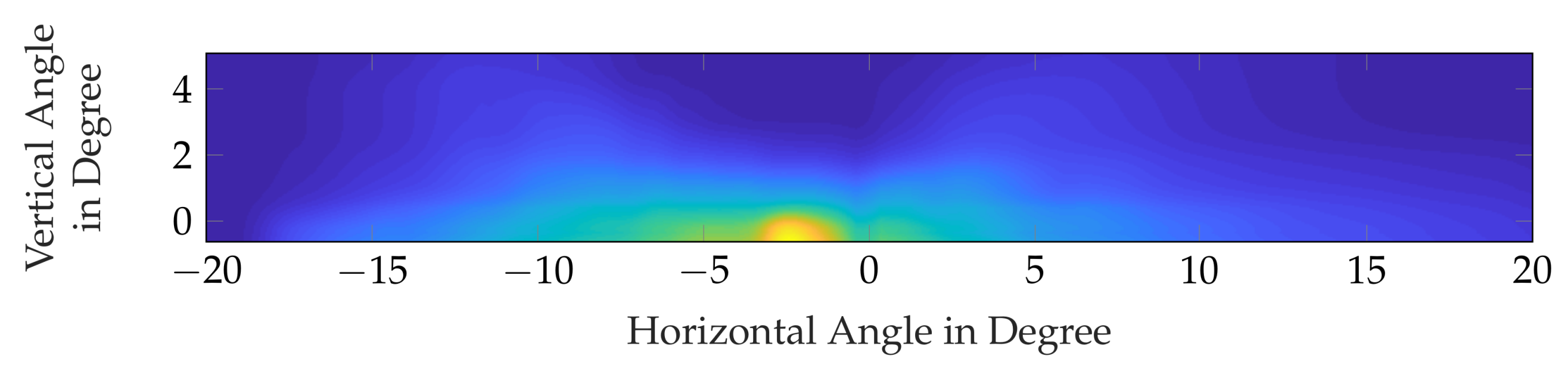
Since all drives and therefore the traffic discussed here were recorded during night, only two major groups of objects were relevant: motor vehicles and traffic signs. Overall the object distributions were as expected. As an example for a typical traffic sign distribution, Figure 4 shows the country road distribution.

Here, it is obvious that most traffic signs that are being approached on country roads are located along the right side of the road. They are first recognized by the camera and algorithm within a certain distance at around 2${}^{°}$ vertically and at around 2${}^{°}$ horizontally. As soon as the vehicle comes closer to the traffic sign, the sign moves toward the top right corner of the camera’s field of view—a normal geometric behavior.

On motorways, this looks fairly similar, but a significant portion of traffic signs is also found above the road with a small proportion also being registered to the left of the road. However, this highly depends on the lane the vehicle is in, as usually a traffic sign that is placed on either side is duplicated on the other side as well. Therefore, the traffic sign distribution is much less pronounced and blurrier.

In cities, traffic signs appear mostly on the right side again, but are placed at much greater vertical variance, blurring the distribution image as well.

When it comes to motor vehicles, the distributions are easily explained. On country roads, the traffic is mostly recognized to the left of the vehicle and directly in front. In the city, due to parked vehicles and the relatively low relative velocity to other vehicles, objects can be recognized almost anywhere in front of the driver’s vehicle.

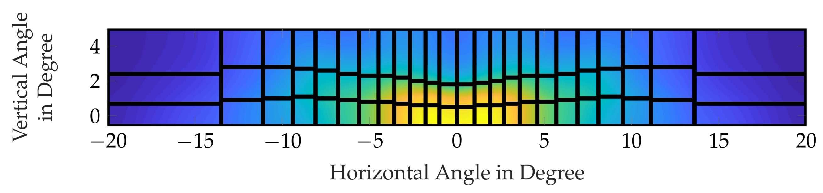
Motor vehicles seem to be the most interesting here. Since the relative velocity to passing vehicles is rather low as well, and similar on the left and right, two major “hot spots” on each side exist. This is shown in Figure 5.

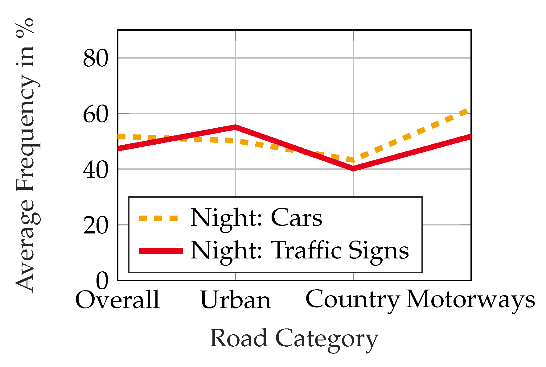
Overall the data show that most objects are found on motorways and in cities. Figure 6 shows the relative number of frames with at least one motor vehicle (orange, dotted line) or one traffic sign (red, solid line) for the three road categories, as well as overall.

A total of 230,000 cars, 9500 trucks, 400 buses, 20 motorbikes and 150,000 traffic signs were recognized and evaluated by the software. It should be noted that this does not mean that 230,000 different cars were recognized nor that there were 230,000 frames with cars. A single car can appear on multiple frames and therefore be counted multiple times into this statistic. At the same time, it is also possible that multiple cars are on one frame and therefore, both count into this statistic as well.

While these data bring no real surprises, it is absolutely necessary to have valid real-life data for the next steps in the light distribution optimization.

3. Segment Optimization for Adaptive Driving Beam

In this section, the data collected and evaluated by object recognition were used to optimize segment sizes of adaptive driving beam (ADB) segments.

Until now, the segments of ADB systems have generally been uniformly distributed with equal sizes over the complete light distribution, with some headlamp manufacturers using wider segments at the outer edges for improved side illumination. However, the goal of this optimization is to select segment sizes that would maximize the usage of adaptive driving beam as proposed by Moisel, Totzauer and authors of this paper [20,21,22].

3.1. Optimization Algorithms and Constraints

As shown by Totzauer, different possibilities and optimization algorithms for this kind of problem exist. The general idea for the proposed optimization is that each area that is illuminated by a segment of the adaptive driving beam should be switched on and off the same percentage of time as all other segments. Since most traffic, due to the relative angular velocity to the camera, is near the center of the light distribution (see Figure 5, slightly offset to the left due to right-hand side driving, those center pixels should be the smallest. Segments at the outer sides of those light distributions are only turned off very briefly since the angular velocity of oncoming and passing traffic under those angles is the highest; therefore, the duration for which a vehicle is present in those areas is the shortest.

For this purpose, the data presented in the sections above were used. As already described in [22], a certain number of adaptive driving beam segments were taken and distributed in rows and columns. This was done for all possible combinations between one single pixel (no optimization possible) to 10,000 pixels.

As a constraint, the segments in each column had to have the same width and each column had to contain the same number of rows. This was done to allow for a somewhat realistic configuration, which could at least in theory be manufactured.

Since adaptive driving beam may not be used inside city limits, the baseline data for the optimization consisted only of the data obtained on country roads and motorways. The data shown in the following had a 60% weight factor for country roads and a 40% weight factor for motorways. This was done since the most common use of adaptive driving beam is on open country roads, where such a light function also is expected to provide the most benefit. However, any weighting of the data is of course possible.

Furthermore, the traffic sign distribution was considered as well. At areas where a traffic sign was recognized by the camera, the segment was dimmed down to 75% intensity, since this was found to be the optimal average intensity [33].

To achieve a segment distribution that could be used in real traffic, another condition was that the overall segment distribution should be symmetrical. This was achieved by additively mirroring the traffic and traffic sign data before optimizing the segment sizes.

3.2. Optimized Segment Distribution

Since it is obviously impossible to show all optimization results, Figure 7 shows an example of such an optimized segment distribution for a (3 × 24)-segment high beam.

Inspection of this figure clearly illustrates the initial hypothesis that the more vehicles are recognized under a certain angle, the smaller these segments need to be. Since the highest frequency of registered objects was found near the center of the light distribution, this is where the smallest segments are found as well. The largest segments were found all the way at ±20${}^{°}$ horizontally and 2${}^{°}$ upwards vertically. (One could also argue that no light is actually necessary under those angle positions because it would be unlikely that a driver needs to respond to an object at these positions).

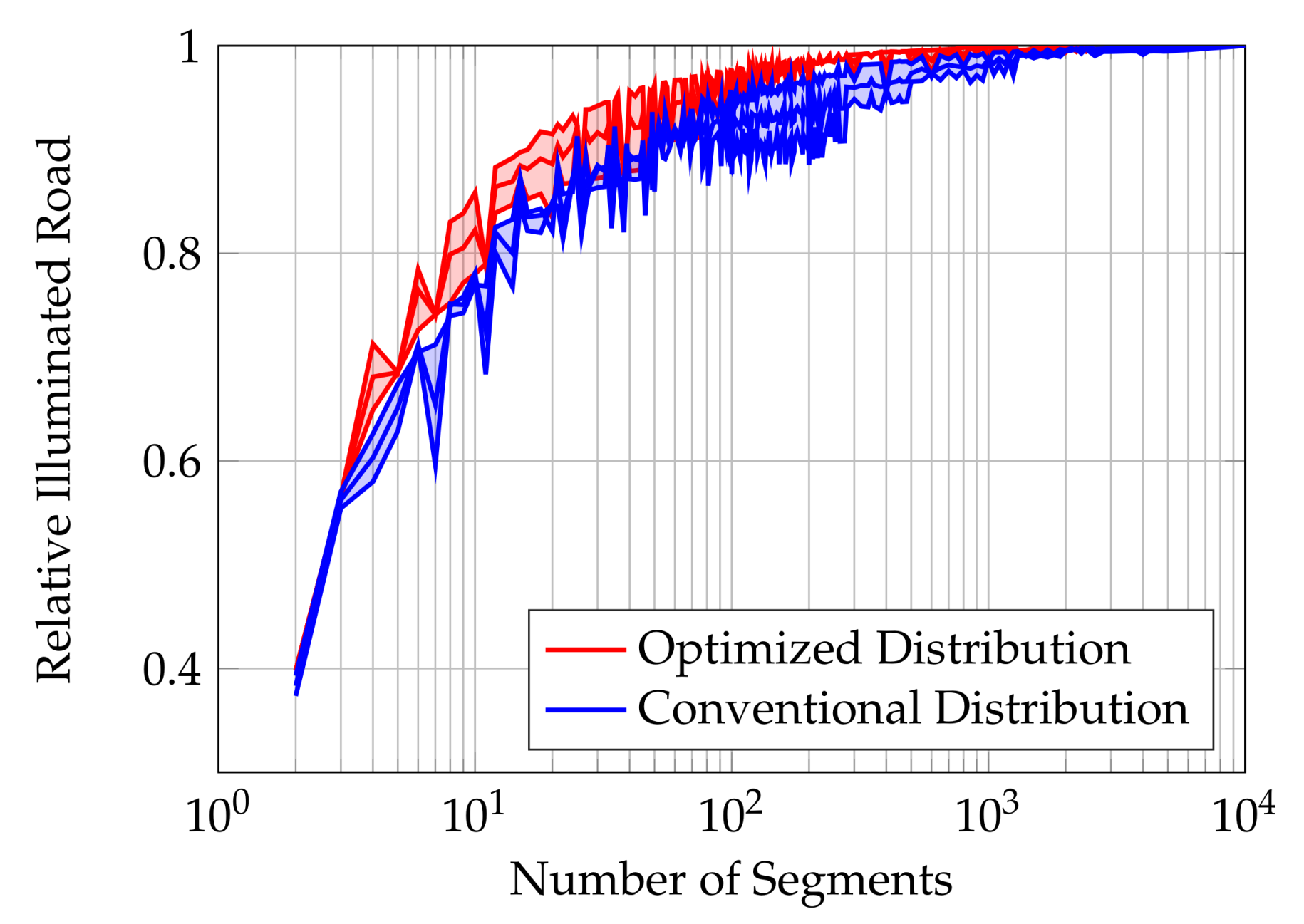
In order to check if the optimization led to any benefit, all nonoptimized light segment distributions as well as all optimized light distributions were tested against a set of 2000 test frames. For each of these frames randomly selected from the country road and motorway data, the number of active segments was recorded and the percentage of the illuminated area was calculated. This is shown in Figure 8.

While both curves seem to be rather similar, it is directly obvious that the optimized segment distribution always performed at least as well or better than the conventional distribution by having a larger proportion of road area being illuminated to a higher level. While this was not a perfect test to ensure that the optimization algorithm was ideal, the fact that the algorithm resulted in more illumination directed to safety-critical locations and the fact that the performance became asymptotic beyond 100–1000 segments were very promising that the algorithm’s sensitivity and accuracy was sufficient for this purpose. The high variance for certain segment numbers is explained by the possibility to form different patterns with a certain number of pixels. One hundred pixels can, for example, be set to a (10 × 10)- or a (2 × 50)-segment distribution. For those cases, the lowest, highest, and mean illumination levels are shown.

The second thing to note in this figure is that the higher the number of segments, the lesser the impact of such an optimized light distribution.

Furthermore, the figure also shows a diminishing return of illuminated road area for headlamps with more than 1000 segments. However, this is only for the purpose of illuminating objects to be seen along the road. Such higher-segment headlights can of course bring other benefits in the form of a high-resolution road projection or light-based driver assistance systems.

Overall, the data here show that there can be certain benefits to the overall approach. However, the theoretical analysis as shown in [22] has highlighted more potential with higher projected benefits by the optimization. The general way the optimized segments are sorted, however, remains the same as predicted. Nevertheless, it was important to show that this approach also works with real-life data.

4. Discussion

With the goal of optimizing modern headlight distributions based on gaze behavior and current traffic analysis, this paper described the second of three parts of our research. We analyzed a total of 54 test drives, each over 100 km long consisting of urban roads, country roads and motorways.

Although the overall result of these traffic distributions collected during this investigation was as expected, it was rather important to update these data to the current road and traffic conditions. Furthermore, this part of the research set the base for the subsequent gaze behavior analysis by setting up the test vehicle and the driven route.

In the last part of this paper, the arrangement of segments for adaptive driving beam headlamps was optimized based on the data acquired during this research. The results here showed a small but noticeable improvement on road illumination if the optimization approach as suggested were used with a number of segments, rather than swiveling headlights or other legacy approaches.

In general, one major limitation of the present approach is that only one route was selected, and thereby, the generalization to all European roads, and even less to roads on other continents, has to be questioned. However, for this particular research, this step was necessary, as the next step, analyzing the gaze behavior, requires similar situations for all test subjects in order to be comparable.

Another thing to consider is that the development of machine learning algorithms, including object recognition software, is expected to improve with each year. For this reason, updating the database and extending it, not only by adding more video data, but evaluating it with new and improved algorithms can lead to more stability and more reliable datasets in the future.

This paper can be thought of in two ways: as a description for an analytical step in developing new headlight beam patterns or confirming the utility of existing ones, and as an empirical basis for describing real-world roadway environments in Germany (and hopefully, beyond). It is important to emphasize that while the latter purpose indeed has some limitations, the former purpose is the primary outcome of this work and can be applied to additional, more extensive descriptive data. Indeed, this is our hope.

References

- Damasky, J. Geometry of the Road Area and Effects on Motor Vehicle Lighting. In Proceedings of the Symposium Progress in Automobile Lighting, PAL, Darmstadt, Germany, 1995; Volume 7. [Google Scholar]
- Schulz, R. Blickverhalten und Orientierung von Kraftfahrern auf Landstraßen. Ph.D. Thesis, Technische Universität Dresden, Dresden, Germany, 2012. [Google Scholar]
- Schwab, G. Untersuchungen zur Ansteuerung Adaptiver Kraftfahrzeugscheinwerfer. Ph.D. Thesis, Technische Universität Ilmenau, Ilmenau, Germany, 2003. [Google Scholar]
- Kuhl, P. Anpassung der Lichtverteilung an den Vertikalen Straßenverlauf. Ph.D. Thesis, Universität Paderborn, Paderborn, Germany, 2006. [Google Scholar]
- European Automobile Manufacturers Association. ACEA Report—Vehicles in Use. 2021. Available online: https://www.acea.auto/publication/report-vehicles-in-use-europe-january-2021/ (accessed on 12 December 2021).
- United Nations Economic Commission for Europe. Uniform Provisions Concerning the Approval of Adaptive Front-Lighting Systems (AFS) for Motor Vehicles, Revision 2; Technical Report; UNECE: Geneva, Switzerland, 2013. [Google Scholar]
- Huhn, W. Anforderungen an Eine Adaptive Lichtverteilung für Kraftfahrzeugscheinwerfer im Rahmen der ECE-Regelungen. Ph.D. Thesis, Technische Universität Darmstadt, Darmstadt, Germany, 1999. [Google Scholar]
- Müller, N.; Waldner, M.; Bertram, T. Virtual Development and Optimization of High-Definition Headlights. In Proceedings of the 2022 International Conference on Electrical, Computer, Communications and Mechatronics Engineering (ICECCME), Maldives, Maldives, 16–18 November 2022; pp. 1–6. [Google Scholar] [CrossRef]
- Rosenhahn, E.O. Fog Headlamp-Visibility Investigations and Performance Requirements for Redefinition in Adaptive Headlamp Systems. In Proceedings of the SAE 2003 World Congress & Exhibition, SAE International, USA, 3 March 2003; Available online: https://www.sae.org/publications/technical-papers/content/2003-01-0555/ (accessed on 11 April 2023).
- Rajesh Kanna, S.K.; Lingaraj, N.; Sivasankar, P.; Raghul Khanna, C.K.; Mohanakrishnan, M. Optimizing Headlamp Focusing Through Intelligent System as Safety Assistance in Automobiles. In Advances in Manufacturing Technology; Hiremath, S.S., Shanmugam, N.S., Bapu, B.R.R., Eds.; Springer: Singapore, 2019; pp. 533–545. [Google Scholar]
- Erkan, A.; Hoffmann, D.; Kreß, N.; Vitkov, T.; Kunst, K.; Peier, M.A.; Khanh, T.Q. Required Visibility Level for Reliable Object Detection during Nighttime Road Traffic in Non-Urban Areas. Appl. Sci. 2023, 13, 2964. [Google Scholar] [CrossRef]
- Reagan, I.J.; Brumbelow, M.L. Drivers’ detection of roadside targets when driving vehicles with three headlight systems during high beam activation. Accid. Anal. Prev. 2017, 99, 44–50. [Google Scholar] [CrossRef]
- Funk, C.; Vozza, A.; Petroskey, K. An Optimized Method for Mapping Headlamp Illumination Patterns. In Proceedings of the SAE WCX Digital Summit. SAE International, USA, 2021; Available online: https://saemobilus.sae.org/content/2021-01-0886/ (accessed on 11 April 2023).
- Reagan, I.J.; Brumbelow, M.; Frischmann, T. On-road experiment to assess drivers’ detection of roadside targets as a function of headlight system, target placement, and target reflectance. Accid. Anal. Prev. 2015, 76, 74–82. [Google Scholar] [CrossRef] [PubMed]
- Reagan, I.J.; Frischmann, T.; Brumbelow, M.L. Test track evaluation of headlight glare associated with adaptive curve HID, fixed HID, and fixed halogen low beam headlights. Ergonomics 2016, 59, 1586–1595. [Google Scholar] [CrossRef] [PubMed]
- Waldner, M.; Müller, N.; Bertram, T. Energy-Efficient Illumination by Matrix Headlamps for Nighttime Automated Object Detection. Int. J. Electr. Comput. Eng. Res. 2022, 2, 8–14. [Google Scholar] [CrossRef]
- Cengiz, C.; Kotkanen, H.; Puolakka, M.; Lappi, O.; Lehtonen, E.; Halonen, L.; Summala, H. Combined eye-tracking and luminance measurements while driving on a rural road: Towards determining mesopic adaptation luminance. Light. Res. Technol. 2014, 46, 676–694. [Google Scholar] [CrossRef]
- Winter, J.; Fotios, S.; Völker, S. The effect of assuming static or dynamic gaze behaviour on the estimated background luminance of drivers. Light. Res. Technol. 2019, 51, 384–401. [Google Scholar] [CrossRef]
- Erkan, A.; Babilon, S.; Hoffmann, D.; Singer, T.; Vitkov, T.; Khanh, T.Q. Determination of Speed-Dependent Roadway Luminance for an Adequate Feeling of Safety at Nighttime Driving. Vehicles 2021, 3, 821–839. [Google Scholar] [CrossRef]
- Moisel, J. Adaptive Headlights Utilizing LED-Arrays. In Proceedings of the 8th International Symposium on Automotive Lighting (ISAL 2009), Darmstadt, Germany, 29–30 September 2009; Herbert Utz Verlag: Munich, Germany, 2009; Volume 13, pp. 287–296. [Google Scholar]
- Totzauer, A. Erarbeitung einer Effizienten Fernlichtunterteilung Abgeleitet aus einem Stochastischen Modell der Bedingungen des Deutschen Straßenverkehrs. Studienarbeit. 2008. Available online: https://tubiblio.ulb.tu-darmstadt.de/53695/ (accessed on 11 April 2023).
- Kobbert, J.; Kosmas, K.; Khanh, T. Glare-free high beam optimization based on country road traffic simulation. Light. Res. Technol. 2019, 51, 922–936. [Google Scholar] [CrossRef]
- Cordts, M.; Omran, M.; Ramos, S.; Rehfeld, T.; Enzweiler, M.; Benenson, R.; Franke, U.; Roth, S.; Schiele, B. The Cityscapes Dataset for Semantic Urban Scene Understanding. In Proceedings of the IEEE Conference on Computer Vision and Pattern Recognition, Las Vegas, NV, USA, 27–30 June 2016; pp. 3213–3223. [Google Scholar]
- Martín, A.; Agarwal, A.; Barham, P.; Brevdo, E.; Chen, Z.; Citro, C.; Corrado, G.; Davis, A.; Dean, J.; Devin, M.; et al. TensorFlow: Large-scale Machine Learning on Heterogeneous Systems. 2015. Available online: http://tensorflow.org/ (accessed on 12 February 2018).
- Adamy, J. Fuzzy Logik, Neuronale Netze und Evolutionäre Algorithmen; Shaker Verlag: Herzogenrath, Germany, 2011. [Google Scholar]
- Girshick, R.; Donahue, J.; Darrell, T.; Malik, J. Rich Feature Hierarchies for Accurate Object Detection and Semantic Segmentation. In Proceedings of the IEEE Conference on Computer Vision and Pattern Recognition (CVPR), Columbus, OH, USA, 23–28 June 2014; pp. 580–587. [Google Scholar]
- Krizhevsky, A.; Sutskever, I.; Hinton, G.E. Imagenet Classification with Deep Convolutional Neural Networks. In Proceedings of the Advances in Neural Information Processing Systems, Lake Tahoe, NV, USA, 3–6 December 2012; pp. 1097–1105. [Google Scholar]
- Huang, J.; Rathod, V.; Sun, C.; Zhu, M.; Korattikara, A.; Fathi, A.; Fischer, I.; Wojna, Z.; Song, Y.; Guadarrama, S.; et al. Speed/Accuracy Trade-Offs for Modern Convolutional Object Detectors. In Proceedings of the 2017 IEEE Conference on Computer Vision and Pattern Recognition (CVPR), Honolulu, HI, USA, 21–26 July 2017; Volume 4. [Google Scholar]
- Pkulzc. Tensorflow Detection Model ZOO. 2017. Available online: https://github.com/tensorflow/models/blob/master/research/object_detection/g3doc/detection_model_zoo.md (accessed on 18 July 2018).
- Open Street Map. Open Street Map—Wiki—Special Road Types. 2021. Available online: https://wiki.openstreetmap.org/wiki/Key:highway#Special_road_types (accessed on 13 December 2021).
- Pratt, M.P.; Bonneson, J.A.; Miles, J.D. Measuring the Non–Circular Portions of Horizontal Curves: An Automated Data Collection Method Using GPS. In Proceedings of the Transportation Research Board 90th Annual Meeting, Washington, DC, USA, 23–27 January 2011. [Google Scholar]
- Ai, C.; Tsai, Y. Automatic Horizontal Curve Identification and Measurement Method Using GPS Data. J. Transp. Eng. 2014, 141, 401–408. [Google Scholar] [CrossRef]
- Kosmas, K.; Kobbert, J.; Khanh, T.Q. Field-Test to Determine the Optimal Traffic Sign Illumination Based on Glare-Free High Beam. In Proceedings of the 12th International Symposium on Automotive Lighting (ISAL 2017), Darmstadt, Germany, 2017; Khanh, T.Q., Ed.; Volume 17, pp. 185–190. Available online: https://www.utzverlag.de/assets/pdf/44671dbl.pdf (accessed on 11 April 2023).