Abstract
Physically based cloth simulation requires a model that represents cloth as a collection of nodes connected by different types of constraints. In this paper, we present a coefficient prediction framework using a Deep Learning (DL) technique to enhance video summarization for such simulations. Our proposed model represents virtual cloth as interconnected nodes that are subject to various constraints. To ensure temporal consistency, we train the video coefficient prediction using Gated Recurrent Unit (GRU), Long-Short Term Memory (LSTM), and Transformer models. Our lightweight video coefficient network combines Convolutional Neural Networks (CNN) and a Transformer to capture both local and global contexts, thus enabling highly efficient prediction of keyframe importance scores for short-length videos. We evaluated our proposed model and found that it achieved an average accuracy of 99.01%. Specifically, the accuracy for the coefficient prediction of GRU was 20%, while LSTM achieved an accuracy of 59%. Our methodology leverages various cloth simulations that utilize a mass-spring model to generate datasets representing cloth movement, thus allowing for the accurate prediction of the coefficients for virtual cloth within physically based simulations. By taking specific material parameters as input, our model successfully outputs a comprehensive set of geometric and physical properties for each cloth instance. This innovative approach seamlessly integrates DL techniques with physically based simulations, and it therefore has a high potential for use in modeling complex systems.
1. Introduction
Cloth simulation is an advanced technique used in computer graphics to generate lifelike animations of fabric materials within virtual environments [1]. By representing cloth as a grid of interconnected particles [2], which are typically connected by springs or constraints [3], its behavior can be realistically simulated by considering its physical properties [4] and its response to external forces. To conduct the simulation, the physical characteristics of the cloth, such as mass, stiffness, damping, and friction, are defined [5,6]. These properties dictate how the cloth will react to various forces and movements. The cloth is typically represented as a mesh composed of vertices and triangles, thus allowing for intricate and detailed simulations.
External forces, including gravity, wind, and collisions with objects or the environment, are then applied to the cloth simulation, which affects the motion and deformation of the cloth [7]. These forces are accurately computed and then exerted upon the cloth’s particles or vertices, thus resulting in an accurate simulation of their movement and interplay. Cloth simulation can be used in a wide variety of applications in computer graphics and animation, particularly in virtual fashion design software, where it can be used to simulate different fabrics and garments, thus enabling virtual try-on experiences and visualizations of clothing movements on virtual avatars [8]. The utility of cloth simulation extends beyond entertainment, as it can be used in product design, engineering, and scientific research, such as by facilitating the evaluation of textile-based product performance, simulating fabric behavior under varying conditions, and aiding in the development of new materials and designs [9].
Cloth simulation [10] is used in a wide range of applications, including video games, recommendation systems, and virtual try-on systems for clothing retailers. This allows designers and animators to create realistic and believable cloth movements that accurately replicate the behavior of real-world clothes [11,12]. Cloth simulations have seen significant increases in their accuracy and complexity in recent years. DL is a subset of machine learning that uses neural networks to analyze and learn from large datasets [13]. DL has been increasingly used in various applications, including computer graphics and cloth simulation. DL techniques can be used to train neural networks to predict the behavior of cloth based on a variety of input factors, including the coefficients of the mass-spring system [14].
In the context of cloth simulation using the mass-spring system, Zorah Lahner et al. [15] presented an original framework consisting of two modules that work jointly to represent both global shape deformation and surface details with high fidelity. In that framework, global shape deformations are recovered from a subspace model that has been learned from 3D data of clothed people in motion, while high-frequency details are added to normal maps created using a conditional Generative Adversarial Network whose architecture has been designed to enforce realism and temporal consistency. Eunjung ju et al. [16] proposed a two-stream fully connected neural network model and proved the suitability of the neural network model by comparing its learning error and accuracy with those of other similar neural networks and linear regression models. Tae Min Lee et al. [17] proposed an efficient cloth simulation method using miniature cloth simulation and upscaling Deep Neural Networks (DNN). In that method, upscaling DNNs generate the target cloth simulation from the results of physically based simulations of a miniature cloth with physical properties that are similar to those of the target cloth.
In another approach, Hugo Bertiche et al. [18] presented a general framework for the garment animation problem that involves unsupervised deep learning inspired by physically based simulation. Artur Grigorev et al. [19] proposed a method that leverages graph neural networks, multi-level message passing, and unsupervised training to enable the real-time prediction of realistic clothing dynamics. One key contribution of that work is a hierarchical message-passing scheme that efficiently propagates stiff stretching modes while preserving local detail.
José E. Andrade et al. [20] proposed a predictive multiscale framework for modeling the behavior of granular materials. That method is particularly attractive due to its simplicity and ability to exploit the existing finite element and computational inelasticity technologies. In addition to improving the accuracy of cloth simulation, DL can also be used to optimize the parameters of the simulation. For example, a neural network can be trained to predict the optimal values of the mass, damping coefficient, and stiffness of the springs, based on the properties of the fabric material [21] and the desired behavior of the simulation. Overall, the combination of the computer simulation using the mass-spring system and DL has the potential to revolutionize cloth simulation and other applications in computer graphics by creating more realistic and accurate simulations of real-world materials and behaviors. Therefore, the key contributions of this paper are as follows:
- The creation of a unique dataset of cloth video simulations from the MMS system, encompassing approximately 1200 videos in each category, totaling around 3600 videos for experimentation across five distinct classes.
- The construction of three foundational models from scratch—GRU, LSTM, and Transformer—to classify the five cloth simulation dataset classes.
- The use of GPU-based fine-tuning of ResNet50, the highest-performing pre-trained model, by integrating it with custom Convolutional Neural Networks (CNN) and Transformer layers.
The rest of this paper is organized as follows: In Section 2, we provide a review of related work in the field of cloth simulation and video classifications using deep learning techniques. In Section 3, we provide a detailed overview of the methodology, dataset simulation, and MMS system overview. In Section 4, we describe the results of implementation and configuration from model experiments. Finally, in Section 5, we conclude by highlighting the potential applications of our method in various domains and suggesting areas for future research.
2. Related Works
Deep learning techniques are powerful tools for predicting or classifying objects. Among these techniques, CNN is particularly adept when used with image or video algorithms due to its exceptional learning power [22]. From traditional architectures like LeNet [23] and AlexNet [24] to more modern ones like DenseNet [25], ResNet [26], Inception-V [27], etc., CNNs have demonstrated excellent performance in a variety of applications. However, the network model’s classification layer in video classification tasks continues to use the soft-max function and cross-entropy loss for back-propagation [28], which can cause the model to become over-fitted and thus degrade the model’s performance. By contrast, The Transformer model is a type of neural network architecture that is commonly used in Natural Language Processing (NLP) [29] tasks, but it can also be used in deep learning techniques such as object classification [30], images recognition [31], speech recognition [32], and sequence modeling [33].
In recent years, there have been several notable works combining CNN and transformer techniques. These methods generally fall into two categories: the direct feeding of image data into a CNN-Transformer model to enhance operability and generality, and novel frameworks that bridge CNN and transformers. For example, in [34], a new framework called CoTr was introduced to combine a CNN and a Transformer for precise 3D medical image segmentation. This framework uses a CNN to extract feature representations, while a Deformable Transformer (DeTrans) efficiently models long-range dependencies on the extracted feature maps.
Yuyan Meng et al. [35] proposed a transfer learning and attention mechanism in the ResNet model to classify and identify violent images, achieving an improved network model with an average accuracy rate of 92.20% for quick and accurate identification of violent images, thus reducing manual identification costs and supporting decision-making against rebel organization activities. Atiq ur Rehman et al. [36] present a comprehensive survey paper examining the success of DL models in automated video classification. In that paper, they discuss the challenges existing in the field, highlight benchmark-based evaluations, and provide summaries of benchmark datasets and performance evaluation metrics.
Moumita Sen Sarma et al. [37] proposed a novel scratch model that combined CNN and LSTM for the accurate classification of Traditional Bangladeshi Sport Videos (TBSV). They created a new dataset specifically for TBSV that comprised five classes, and they used a transfer learning approach by fine-tuning VGG19 and LSTM for classification. Francisco Reinolds et al. [38] compared audio and video analysis for real-time violence detection. They utilized the CRISP-DM methodology and PyTorch models and achieved robust results. They found that video analysis significantly outperformed audio analysis, with video models achieving an average accuracy of 89% compared to the corresponding value of 76% for audio models.
Roberta VrsKova et al. [39] introduced an advanced method for human activity recognition by combining 3DCNN with ConvLSTM layers. Their goal was to optimize the traditional 3DCNN and propose a novel model that seamlessly integrated ConvLSTM layers for real-time human activity recognition. The incorporation of supplementary sensor data has the potential to further enhance their proposed model’s performance. In another study, Shan Yang et al. [40] revolutionized image understanding by introducing an innovative technique for extracting the material properties of cloth from video data. Their approach accurately infers physical characteristics by capturing dynamic variations in cloth appearance. By leveraging CNN and LSTM neural network architectures, they achieved remarkable success in recovering cloth properties from video inputs.
3. Proposed Methods
This section presents a comprehensive methodology for the proposed approach while highlighting its key components. Our model, as shown in Figure 1, utilizing the ResNet50 model as its foundation, requires input as a 3D tensor with a size of 224 × 224 × 3 for color images to be introduced to the model for training and classification, and has been pre-trained on ImageNet to leverage its weights. We use the GRU, LSTM, and Transformer models to evaluate this model. Building upon ResNet50 CNN as a solid base with pre-trained weights, we incorporate transfer learning techniques by incorporating three fully connected layers. We then train our model on the labeled cloth videos dataset to achieve optimal performance.
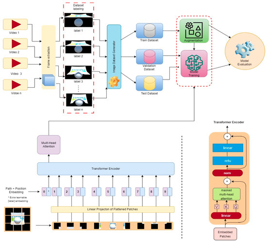
Figure 1.
A CNN-Transformer model is proposed for training and evaluation, as depicted in the block diagram. It involves splitting an image into fixed-size patches, linearly embedding each patch, adding position embeddings, and then feeding the resulting sequence of vectors to a standard transformer encoder. To enable classification, the standard approach of including an additional learnable “classification token” in the sequence is used.
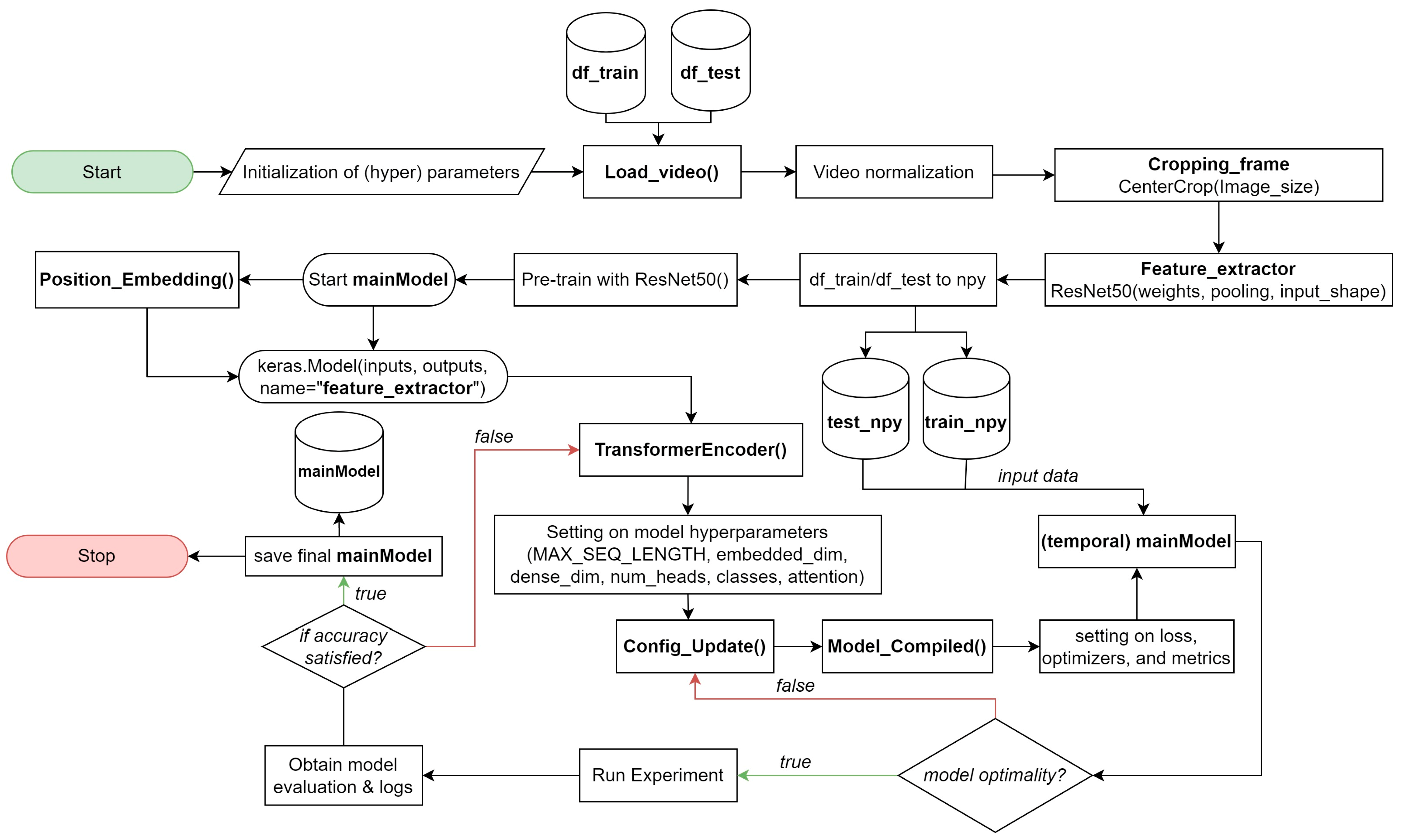
The process flow of our video classification model, as presented in Figure 2, starts with importing the necessary libraries and initializing hyperparameters. We use Python’s TensorFlow and Keras libraries in building and training the model. Hyperparameters (e.g., batch size, learning rate, and the number of epochs) are set at this stage to control the training process. Next, we proceed with loading and preprocessing the video frames for feature extraction. The video frames are normalized to ensure consistent intensity levels across different videos. Moreover, to focus on the most relevant information, we crop the center of each video frame using the “Cropping_frame()” function.
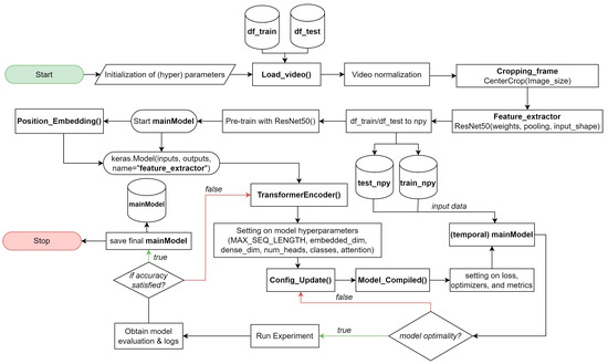
Figure 2.
Process Flow of Video Classification model using Transformer model.
Next, we introduce the feature extraction step, where a pre-trained ResNet50 model is utilized. This ResNet50 model acts as a feature extractor, transforming each video frame into a compact representation that captures essential visual information. The “Feature_extractor” function is responsible for extracting features, and the resulting model is saved as a NumPy file for later use. With the feature extraction process completed, we move on to defining the main model, which incorporates the Transformer architecture. Our Transformer-based model consists of two custom layers: “PositionalEmbedding()” and “TransformerEncoder()”.
The “PositionalEmbedding()” layer plays an important role in adding positional information to the input sequence, which is essential for the Transformer model to understand the temporal ordering of video frames. By including positional embeddings, our model gains temporal awareness, which allows it to achieve better video classification performance. The core of the Transformer model is in the “TransformerEncoder()” layer, which performs self-attention and feedforward transformations. Self-attention allows the model to attend to different parts of the input sequence when making predictions, thereby allowing it to focus on the most relevant frames at different time steps. The feedforward transformation helps capture complex relationships and patterns between video frames.
The “TransformerEncoder()” layer is highly customizable and includes several hyperparameters: (1) MAX_SEQ_LENGTH: controls the maximum number of frames that the Transformer can process in a single video sequence. Sequences longer than this length will be truncated or padded to fit this limit. (2) embed_dim: determines the dimension of the embedded feature representations output by the self-attention mechanism. (3) dense_dim: controls the number of units in the intermediate dense layer, providing flexibility in the model’s capacity. (4) num_heads: indicates the number of attention heads used in the multi-head attention mechanism. The use of a higher number of attention heads can capture more fine-grained relationships within the video frames.
Further, the “classes” parameter represents the number of unique classes or categories that are present in the video classification dataset, which is crucial for determining the output layer’s dimensionality and correctly predicting the video’s class. The “attention” layer within the “TransformerEncoder()” implements the self-attention mechanism with multiple attention heads and enables the model to focus on different parts of the video sequence during training, thus contributing to better learning and representation of complex patterns.
For convenient serialization and later recreation of the “TransformerEncoder()” layer, we implement the “Config_Update()” method, which returns a dictionary containing the layer’s configuration. This allows us to save and load the model architecture along with custom properties such as embed_dim, dense_dim, num_heads, etc. Once the model architecture is established, we compile the model using the “Model_Compiled()” function. The sparse categorical cross-entropy loss function is chosen for video classification tasks, as it can efficiently handle datasets with multiple classes while avoiding the need for one-hot encoding. The Adam optimizer is used to optimize the model parameters during training. After compiling the model, the practical training process is initiated. The model is trained on labeled video data, and the training progress and performance metrics are logged for analysis. During training, we typically monitor several metrics, including accuracy, loss, and validation.
Following training, we evaluate the model on a separate test dataset to assess its generalization performance. This evaluation provides insight into how well the model performs on unseen data and also helps us identify potential overfitting problems. As a final step, we save the trained model along with its weights and architecture, which allows us to reuse the trained model to make predictions on new videos without having to retrain it from scratch.
Our proposed video classification workflow utilizing the Transformer model architecture has the following five advantages over traditional approaches: (1) Long-range Dependency Modeling: The Transformer’s self-attention mechanism enables the model to capture long-range dependencies in video frames. (2) Parallel Processing: Transformers can process video frames in parallel, which significantly speeds up the computation, particularly for longer video sequences with the capability to efficiently analyze and classify videos in real-time or near real-time scenarios. (3) Positional Embeddings: The inclusion of positional embeddings enables the model to understand the temporal ordering of video frames to better recognize actions and events in videos where the sequence of frames matters. (4) Transfer Learning: By utilizing a pre-trained ResNet50 model as a feature extractor, we benefit from transfer learning by leveraging pre-learned visual representations, which can be advantageous when working with a relatively small video classification dataset. (5) Scalability: Our Transformer architecture has demonstrated scalability that is superior to that of traditional RNNs, thus making it more suitable for processing longer videos with complex temporal dynamics.
3.1. Data Set
The mass-spring system (MSS) is a widely used technique in computer graphics that allows for the realistic simulation of cloth and other deformable objects. We collected video of the mass-spring-damper model-based cloth simulation using the GPU-based method in the Unity3D engine. The cloth object is represented by a set of N nodes and M springs.
Therefore, our cloth simulations are made of 32 × 32 nodes with different coefficients to make a difference in each category. Table 1 lists the parameters we used in generating the dataset. Note that velocity damping is used to reduce the elasticity behavior of the cloth. Since the mass-spring-damper model requires a small time step to perform a stable simulation, the animation can be slow. As a result, we increase the animation speed in each simulation loop.

Table 1.
Parameters used to generate cloth dataset.
In addition to the spring constant, the damping coefficient () is another significant factor in the simulation. The damping coefficient controls the rate at which the energy within the spring dissipates. It influences the speed at which the cloth responds to forces and how quickly it settles after disturbances. If the value is excessively high, the cloth exhibits movement that is overly rapid, which makes it appear unstable. The cloth may behave as if it is constantly vibrating or flapping without reaching a state of rest. On the other hand, if the value is set too low, the cloth may oscillate excessively without coming to rest. This means that, even after a disturbance, the cloth takes a very long time to settle down, thus affecting the overall realism of the simulation.
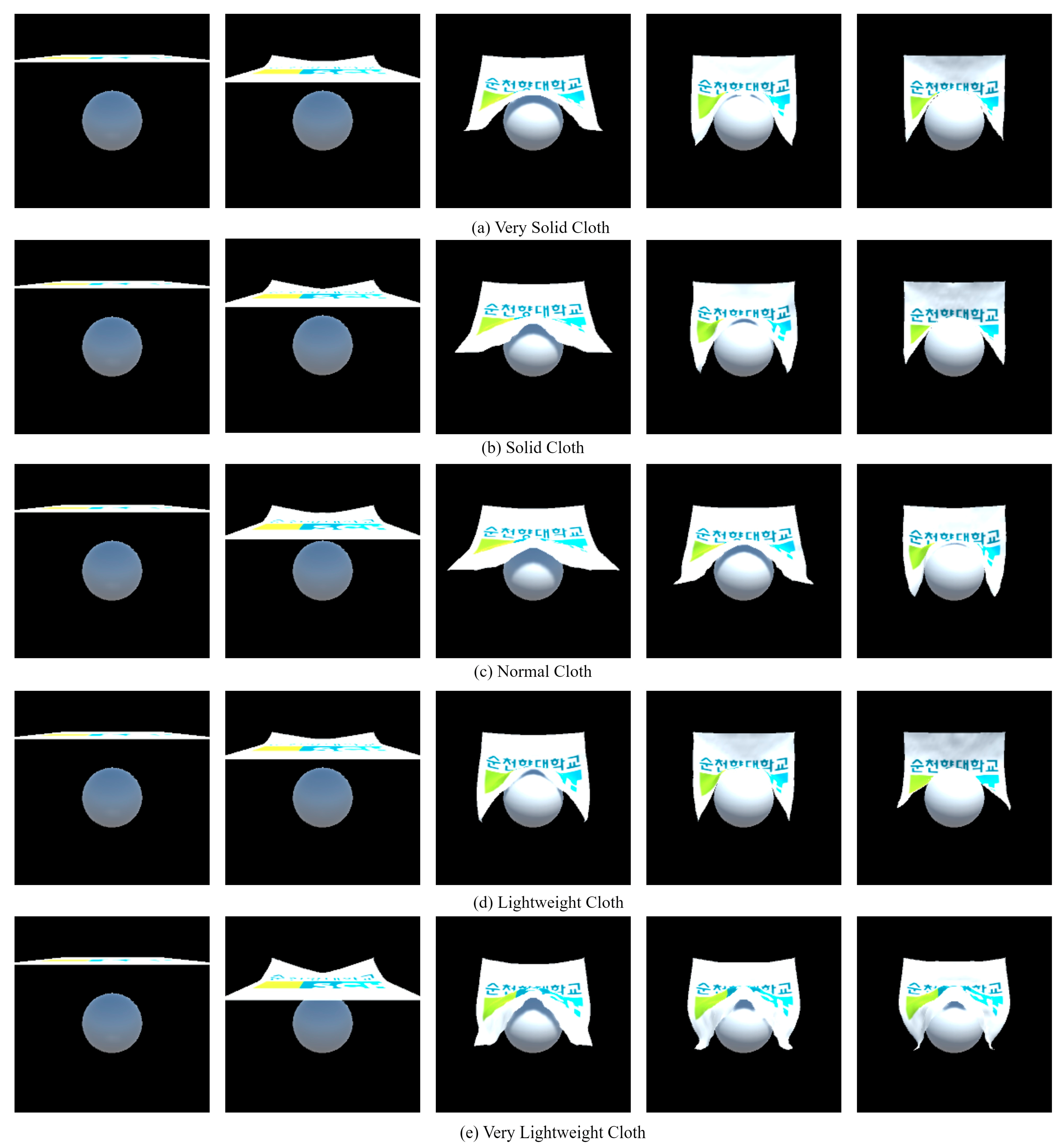
Finding appropriate values for the spring constant () and the damping coefficient () is crucial in achieving a realistic cloth simulation. In this video dataset simulation, as shown in Figure 3. We set to a fixed value of 10 and ranges from 300 to 2000. Specifically, we assigned the value of 300 to represent very lightweight cloth, 800 for lightweight cloth, 1200 for normal cloth, 1600 for solid cloth, and 2000 for very solid cloth.
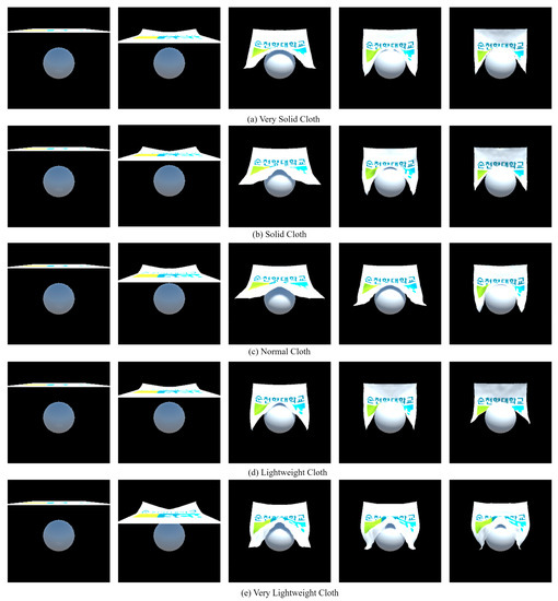
Figure 3.
Demonstrates the skillful manipulation of fabric through the precise repositions of vertical elements to achieve the target positions in demanding tasks.
3.2. Data Augmentation
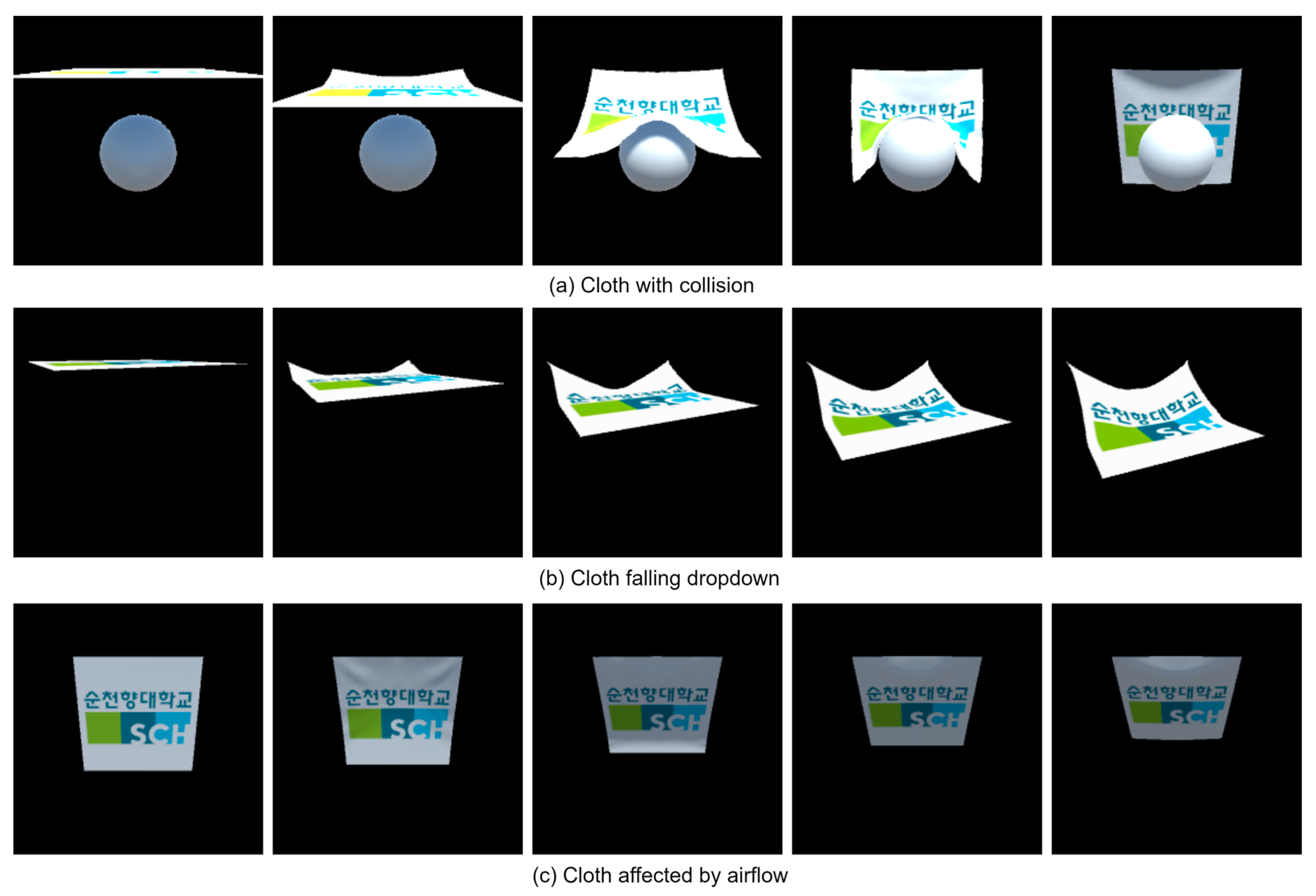
This study investigates the classification of cloths generated from computer simulations while focusing on cloth with collision, cloth falling dropdown, and cloth affected by airflow, as shown in Figure 4. The depth images of these cloths were utilized as input for a DL model to accurately predict their cloth class. Data augmentation is a very important aspect of improving the performance of the model and helping generalize the input data, which reflects better accuracy.
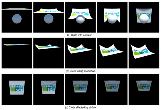
Figure 4.
Animated videos depicting various movements captured from the video dataset. These movements include: (a) cloth with collision; (b) cloth falling dropdown; and (c) cloth affected by airflow.
We used the Keras ImageDataGenerator to augment our training data while applying a range of transformations to enhance the image data. These transformations include scaling, rotation, shearing, adjusting brightness, zooming, channel shifting, width and height shifting, and horizontal and vertical shifting. In our approach, we employed geometric transformations such as rescaling, rotation, width shifting, and height shifting to augment our original dataset for experimentation. In our experimental setup, for each input batch, we randomly applied frame rotation angles of videos ranging from 10 degrees to 50 degrees, along with 20% width and height shifts.
During the data augmentation process, the cloth classes were classified into five distinct groups: very solid cloth, solid cloth, normal cloth, lightweight cloth, and very lightweight cloth. The testing dataset included approximately 400 videos for each category, while the training dataset comprised 875 videos per category. Each video had a duration of 30 s and consisted of 960 frames. In this study, we analyzed a dataset totaling approximately 1275 to 1455 videos per class, and the descriptions of the videos are demonstrated in Table 2.
Table 2.
Dataset used for the video classification experiment.
3.3. Overview of Model
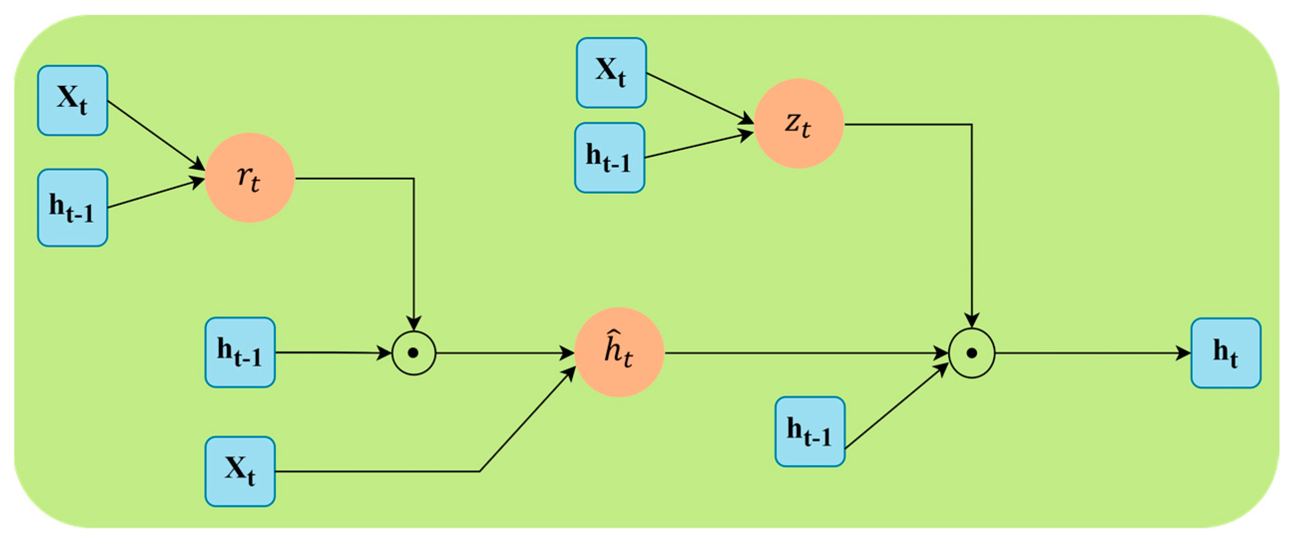
Here, we present an overview of the methods used in this paper and the obtained results. We introduce a novel method with which to compare the existing model with the results obtained from previous experiments, where the GRU model is a type of Recurrent Neural Network (RNN) architecture that is utilized for image and video classification tasks. Having been originally developed as an extension of the standard RNN model, the GRU introduces gating mechanisms to effectively capture and propagate information over sequential data. In the context of image and video classification, the GRU model can be applied sequentially to process the frames or patches of an image or video. This makes the process faster and less memory-consuming, and this model is shown in Figure 5 and described in the equation are given below, where is the reset and update gate, respectively. Meanwhile, is the hidden state.

Figure 5.
Gated Recurrent Unit Architecture.
The GRU does not have direct control over memory content exposure whereas LSTM does have such direct control by having an output gate, as show in Figure 6. These two models differ in how they update the memory nodes. LSTM updates its hidden state by summation overflow after the input gate and forget gate. However, GRU assumes a correlation between how much to keep from the current state and how much to obtain from the previous state, and it models this with the gate.
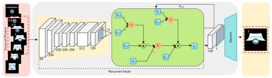
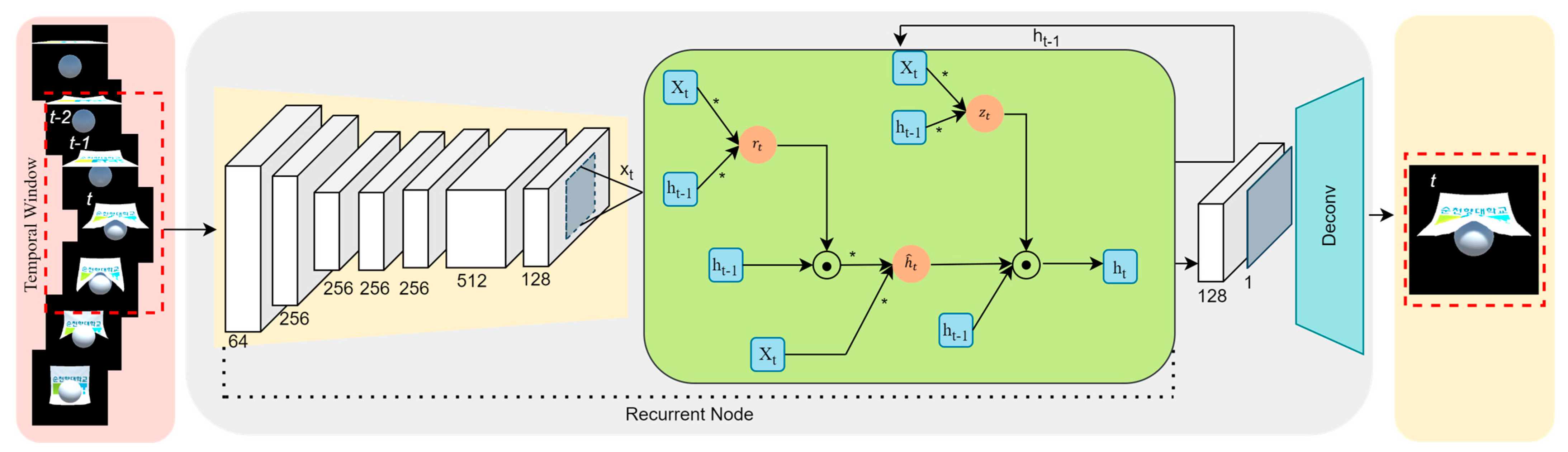
Figure 6.
The architecture utilizes a recurrent full convolutional network with a GRU layer. The image is sequentially fed frame by frame into the network, which consists of a Conv-GRU layer that is applied to the feature maps generated by the preceding network at each frame. * signifies pointwise multiplication. The resulting output is then passed through an additional convolutional layer to generate heat maps. Finally, a deconvolution layer is used to up-sample the heat map to the desired spatial size.
As mentioned above, LSTM uses a gated structure, where each gate controls the flow of a particular signal. Each LSTM node has three gates: input, output, and forget gates, each with learnable weights. These gates can learn the optimal way to remember useful information from previous states and thus decide upon the current state. Equations (5)–(7) shows the procedure of computing different gates and hidden states, where , , and are the input, forget, and output gates, respectively, Equation (9) while denotes the cell’s internal state and Equation (10) is the hidden state.
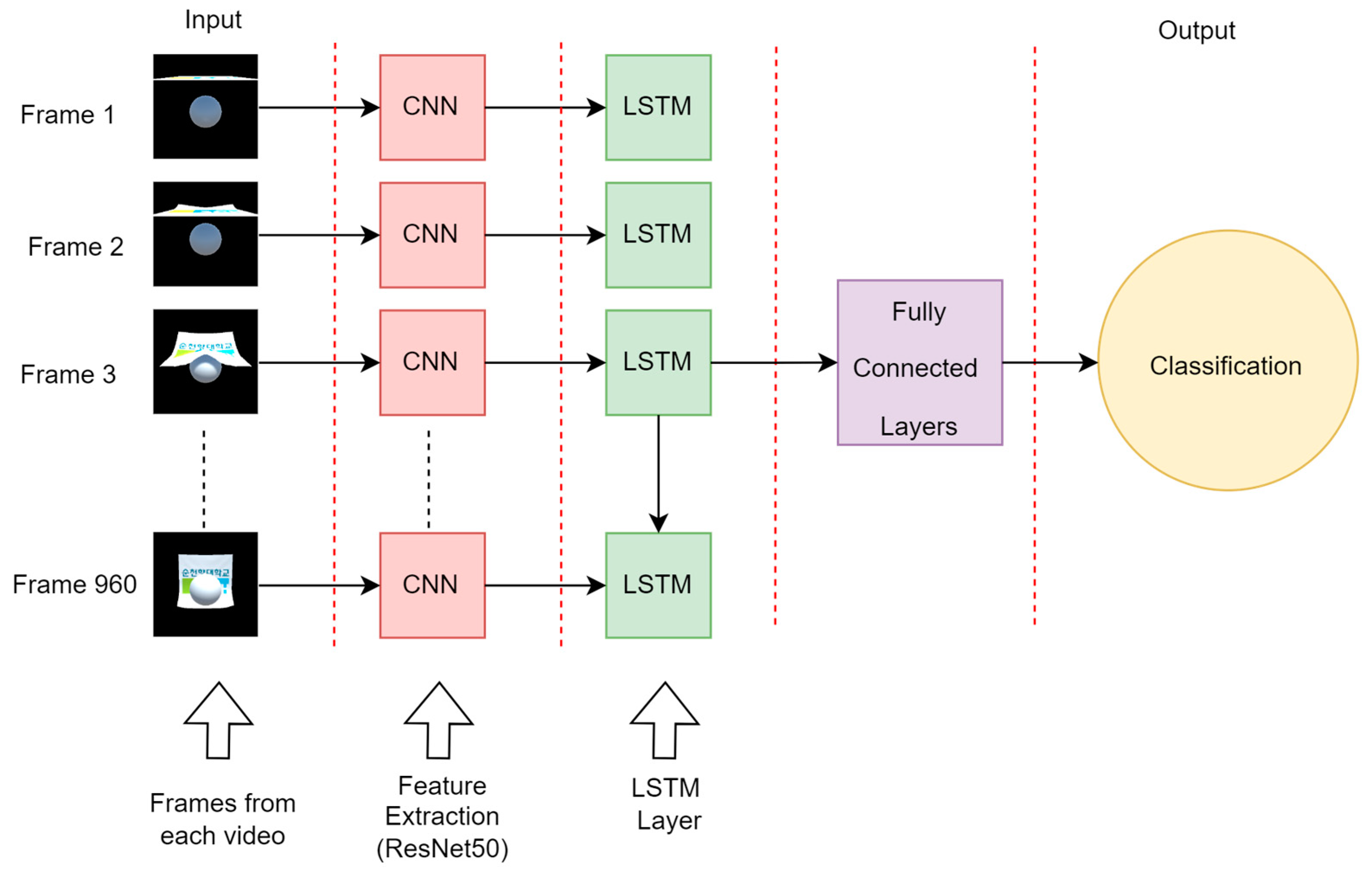
For video classification, the LSTM model follows a sequential processing approach, similar to image classification. This model retains memory cells and hidden states to capture temporal dependencies among frames, which allows it to effectively capture the dynamics and temporal patterns within the video. Therefore, it achieves accurate classification by adeptly learning and representing intricate patterns. In both image and video analysis scenarios, LSTM models consistently deliver precise classification outcomes, as illustrated in Figure 7.

Figure 7.
Illustration of the workflow of video classification using the LSTM model.
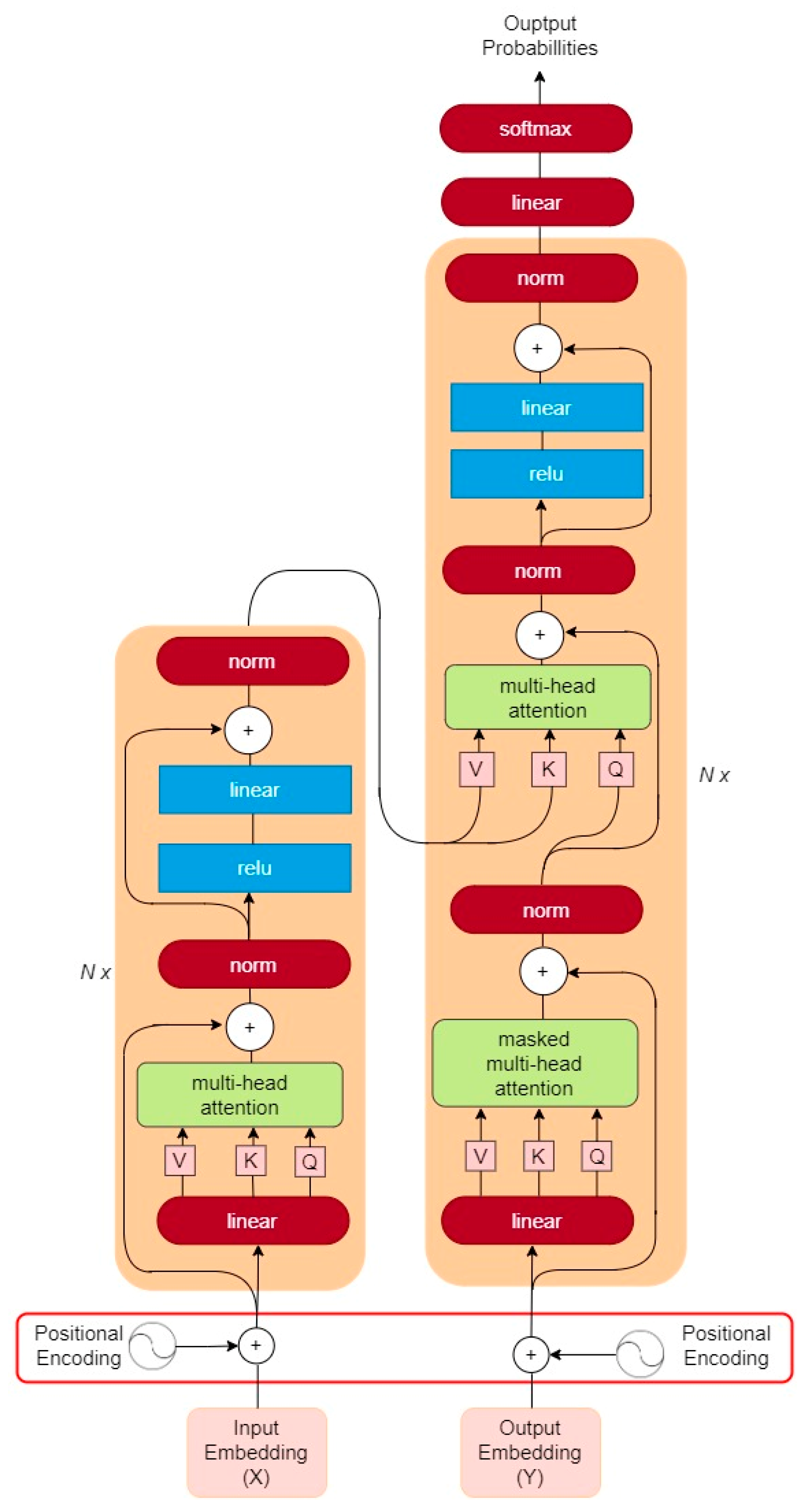
A Transformer model for video classification, as shown in Figure 8, is a hybrid neural network architecture that combines the strengths of CNN and Transformer for the purpose of recognizing and classifying videos. CNNs are particularly effective at processing spatial features in image-based tasks, while Transformers excel at modeling temporal dependencies and capturing long-term context. By combining these two architectures, a CNN-Transformer model can leverage the advantages of both and achieve superior performance in video classification tasks. In such a model, the CNN component is typically responsible for extracting visual features from each frame of the video, and these are fed into the transformer component. The Transformer then models the temporal relationships between the frame and generates a final prediction for the class label of the video. The Transformer model consists of several layers, and each layer consists of two sub-layers: the self-attention mechanism and the feed-forward neural network.
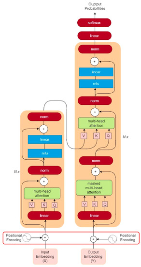
Figure 8.
Given input embeddings and output embeddings . A transformer is typically constructed by stacking encoders linked together. Here, represents the position of the token (token #0, token #1, and so on), denotes the column number of the encoding, and represents the dimension of the encoding (which is equivalent to the dimension of the input embeddings ). This architecture relies solely on attention mechanisms in each encoder and decoder, thus eliminating the need for recurrence or convolutional operations.
During the forward propagation phase, the input data is passed through the self-attention sub-layer, which computes the attention weights between each input element and all other elements in the same layer. This ensures that the model focuses on the important parts of the input while ignoring irrelevant parts. The output of the self-attention, sub-layer is then passed through the feed-forward neural network, which applies non-linear transformations to the data and produces a new representation. During the backpropagation phase, the error signal is propagated backwards through the layers of the network, starting from the output layer, and moving towards the input layer. The error signal is used to update the parameters of the network to allow the model to learn to better classify the objects. For object classification tasks, the Transformer model can be trained using a labeled dataset, where each input is an image, and the corresponding output is the class label of the object in the image. The model can be fine-tuned by optimizing a classification loss function using Stochastic Gradient Descent (SGD), Adam, or other optimization algorithms. The Transformer model is a powerful neural network architecture that can be used for a wide range of tasks, including object classification, and its success is largely attributable to its ability to effectively capture long-range dependencies and learn representations of the input data.
The process flow for Transformer working on video classification is as follows:
- Data Preparation: The first step is to gather and preprocess the video data. This may involve extracting frames from the video, resizing them to a consistent size, and converting them to a format that can be processed by the neural network.
- CNN: The next step is to apply a CNN to each frame in the video to extract visual features. The CNN may consist of several convolutional layers, followed by pooling and activation functions. The output of the CNN is a feature map that represents the most salient visual features of each frame.
- Temporal Encoding: The output of the CNN is then fed into the Transformer component of the models, which models the temporal dependencies between the frames in the video. The Transformer uses self-attention mechanisms to capture long-range dependencies and generate a sequence of encoded features that represents the entire video.
- Classification: Lastly, the encoded features are passed through a fully connected layer to generate a probability distribution over the possible class labels for the video. The class label with the highest probability is selected as the predicted class label for the video.
- Training: The entire model is trained in an end-to-end manner using a suitable loss function such as cross-entropy or spare categorical cross-entropy. The parameters of the model are updated using backpropagation to minimize the loss on a training set of labeled videos.
- Evaluation: The trained model is evaluated on a separate test set of videos to measure its performance in terms of accuracy, precision, recall, and f1 score. The result is used to fine-tune the model and optimize its hyperparameters to achieve better performance.
3.4. Implementation Details
In the proposed model, we introduce an additional fully connected layer for fine-tuning, as show in Pseudocode 1. We leverage the ResNet50 CNN as the foundation model, so it benefits from pre-trained weights and seamlessly appending extra layers without compromising the original weights. To handle these videos, which are sequential in nature, we incorporate positional encoding in the transformer model. This involves embedding the positions of frames using an Embedding layer and adding them to the precomputed CNN feature maps.
In the compiled model, the input shape is defined based on the ‘sequence_length’ obtained from ‘MAX_SEQ_LENGTH’. This value is crucial for padding or truncating the video frames to a fixed length, as it ensures consistent input dimensions for the model. Moreover, the ‘embed_dim’ is set to 2048, which corresponds to the default output dimension of the last pooling layer in ResNet50, which serves as the initial representation for the transformer model.
To incorporate positional information and capture sequential dependencies, the input sequence undergoes a ‘PositionalEmbedding’ layer. This positional embedding is vital for the model to understand the relative order of tokens in the sequence, thus facilitating long-range relationships. Subsequently, a ‘TransformerEncoder’ layer is used to apply the Transformer architecture to the encoded sequence. The TransformerEncoder utilizes self-attention and feedforward neural networks to capture complex relationships within the sequence, therefore allowing the model to recognize relevant patterns and features. To obtain a fixed-length representation of the sequence, a ‘GlobalMaxPooling1D’ layer is applied, which captures the most salient features across the entire sequence. To prevent overfitting during training, dropout regularization is introduced after the pooling layer.
After the pooling and dropout layers, a fully connected dense layer with 32 units and a ReLU activation function is added with the aims of introducing non-linearity to the model and extracting higher-level features. To further mitigate overfitting, an additional dropout regularization is applied before the final output layer. The output layer employs a softmax activation function to generate class probabilities, which allows the model to predict the class label for the input sequence. The model is then compiled using the Adam optimizer, with a learning rate of 0.0001, to facilitate efficient gradient-based optimization. The sparse categorical cross-entropy loss function is chosen for training, as this is suitable for multi-class classification tasks with integer labels. Here, accuracy is used as a metric to monitor the model’s performance during training and validation. To optimize performance and ensure generalization, the model is trained for 250 epochs. A batch size of 32 and a validation split of 0.16 are used during training.
| Pseudocode 1. The architecture of the Transformer model. | ||
| Transformer model architecture | ||
| 1 | def get_compiled_model(): | |
| 2 | sequence_langth = MAX_SEQ_LENGTH | |
| 3 | embed_dim = NUM_FEATURES | |
| 4 | dense_dim = 512 | |
| 5 | num_heads = 2 | |
| 6 | classes = len(label.get_vocabulary()) | |
| 7 | inputs = Input (shape = (sequence_length, embed_dim)) | |
| 8 | x = PositionalEmbedding (sequence_length, embed_dim, name =“frame_position_embedding”) (inputs) | |
| 9 | x = TransformerEncoder(embed_dim, dense_dim, num_heads, name=“transformer_layer”) (x) | |
| 10 | x = layers.GlobalMaxPooling1D() (x) | |
| 11 | x = Dropout(0.5) (x) | |
| 12 | x = Dense(32, activation = ‘relu’) (x) | |
| 13 | x = Dropout(0.5) (x) | |
| 14 | outputs = Dense(classes, activation = ‘softmax’) (x) | |
| 15 | opt = optimizers.Adam(learning_rate = 0.0001) | |
| 16 | model = Model(inputs = inputs, outputs = outputs) | |
| 17 | model.compile(loss = “sparse_categorical_crossentropy”, optimizer = opt, metrics = [“accuracy”]) | |
| 18 | return model | |
| 19 | def run_experiment(): | |
| 20 | model = get_compiled_model() | |
| 21 | history = model.fit( | |
| train_data, | ||
| train_labels, | ||
| validation_data = (test_data, test_labels), | ||
| validation_split = 0.16, | ||
| batch_size = 32, | ||
| epochs = 250) | ||
| 22 | _, test_accuracy = model.evaluate(test_data, test_labels) | |
| 23 | print(f”Test accuracy: {round(test_accuracy * 100, 2)}%”) | |
| 24 | return model | |
The model consists of custom layers, like the Positional Embedding and Transformer Encoder, as well as standard layers, such as Global Max Pooling1D, Dropout, and Densen layers, as show in Table 3. The Positional Embedding layer introduces positional information to the input sequence, which allows the transformer model to capture the order of frames in the video. The Transformer Encoder is the core component that learns to extract relevant features from the video frames. The Global Max Pooling1D layer is used to reduce the temporal dimension, while the Dropout layers help prevent overfitting. Finally, the Dense layers are used for classification, and the model is compiled with the Adam optimizer and spares categorical cross-entropy loss.
Table 3.
Transfer learning—Layer configuration.
Transfer learning has shown promising improvements in training time, saving time for execution and contextual classification. Transfer learning generally reduces training time. In the proposed scenario, all layers of the ResNet50 pre-trained network remained unchanged, and the complete model was employed. We loaded the pre-trained weights and also appended new fully connected layers.
The video source is an MPEG-4 digital recording of the full-length match, encompassing all the features represented by the computer simulation on cloth. A video is composed of frames, which are images of the same size as the video display. To process the video, frames are extracted individually, i.e., one at a time. We extracted frames at a rate of 32 frames per second, thus resulting in a total of 960 frames for a 30-s video. These frames were obtained in high resolution. Before inputting them into the classification system, we resized the frames to match the model’s input shape of 224 × 224 × 3. The frames were pre-conditioned and set in RGB color space before being fed into the input layer of the classifier model. During the frame extraction process, it took approximately seven to eight days to complete each category. The extracted frames were saved as NumPy files for computation during model training.
4. Experiments
4.1. Experimental Setup
We conducted our experiment on a computer equipped with an AMD Ryzen 9 5900x CPU operating at a Core Speed of 3599.16 MHz, and an NVIDIA GeForce RTX 4090 GPU with 24 GB of operating memory. The code was implemented in Python using TensorFlow with the Keras application and the CUDA library for accelerated training. The training process used the Adam optimizer with a learning rate of 0.0001 and a batch size of 32. We utilized the sparse categorical cross-entropy loss model as the performance metric and conducted the training solely on the GPU. Please refer to Table 4 for comprehensive information on devices, software, and parameters, as well as simulation parameters.
Table 4.
Software and Simulation Parameters.
4.2. Results
The results section showcases the experimental evaluations of the performance of our proposed methodology. In the subsequent part, we will provide a comprehensive analysis and discussion of these results. Our evaluation process involved assessing the precision, recall, accuracy, and F1-score for all categories within the video dataset. The effectiveness of video classification relies on the learning capabilities of the network and the specific models and cloth dataset utilized. To compare classification performance, we conducted experiments using three models: GRU, LSTM, and Transformer, on various video datasets. All models were trained for 250 epochs with a training sample of 400 videos. The transformer model was found to outperform the other mentioned models, as it achieved the highest accuracy. Specifically, the transformer achieved an impressively high accuracy of over 99.01% with 1275 video datasets, as show in Table 5. For training, our models were pre-trained on ResNet50. Unless otherwise specified, we utilized 32-image input clips to fine-tune our models. These clips were generated by randomly selecting 64 consecutive frames from the original full-length video and excluding frames with a spatial size of 224 × 224 pixels.
Table 5.
Comparison of classification performance for three different types of cloths using transfer model: cloth with collision, cloth falling down, and cloth affected by airflow.
Regarding the training and evaluation of our proposed method, the image dataset was fed to the training classifier in batches of 32 images, and we parameterized the generator to apply a set of transformations such as flipping, rotating, and shifting in both dimensions to the input images. We partitioned the dataset into 70% for training and 30% for testing, with an additional 16% set aside as a validation dataset within the training data. The training process achieved a robust accuracy of 99.01% after 250 epochs, as shown in Figure 9. Figure 10, Figure 11 and Figure 12 show the training history of the model.
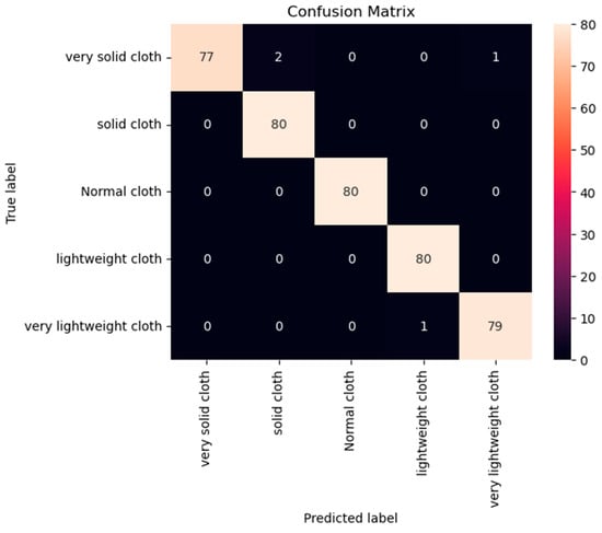
Figure 9.
Confusion Matrix from our experiment dataset on cloth with collision.
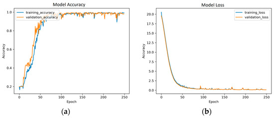
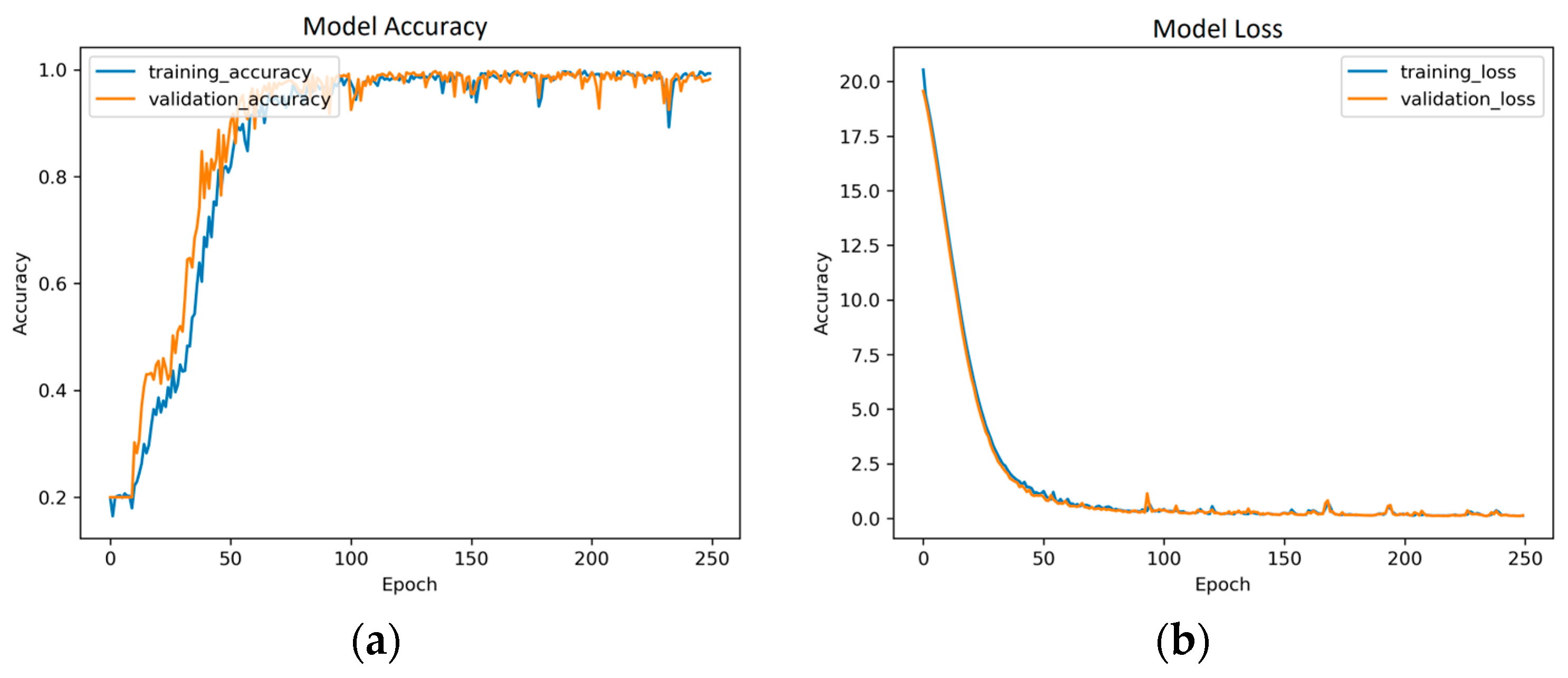
Figure 10.
Proposed model training history from cloth with collision: (a) Model accuracy; (b) Model loss.
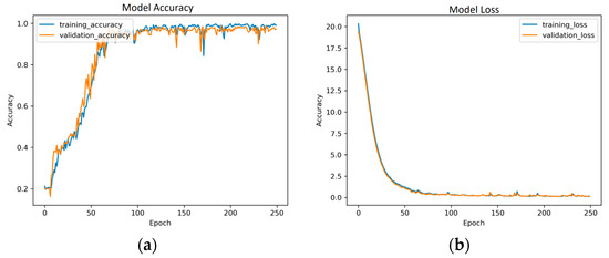
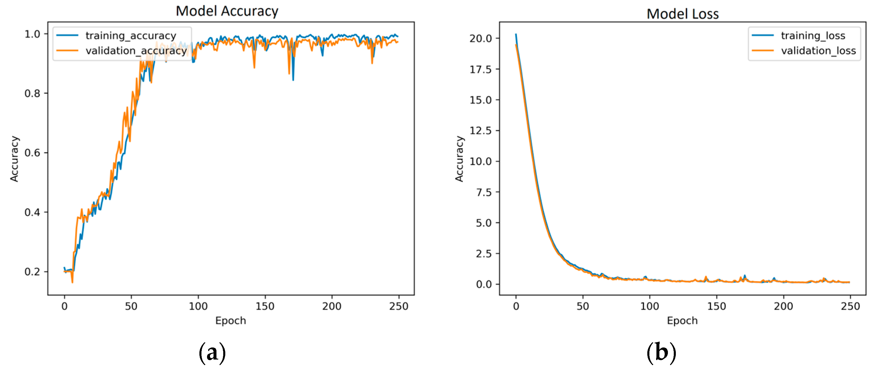
Figure 11.
Proposed model training history from cloth with dropdown: (a) Model accuracy; (b) Model loss.
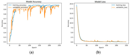
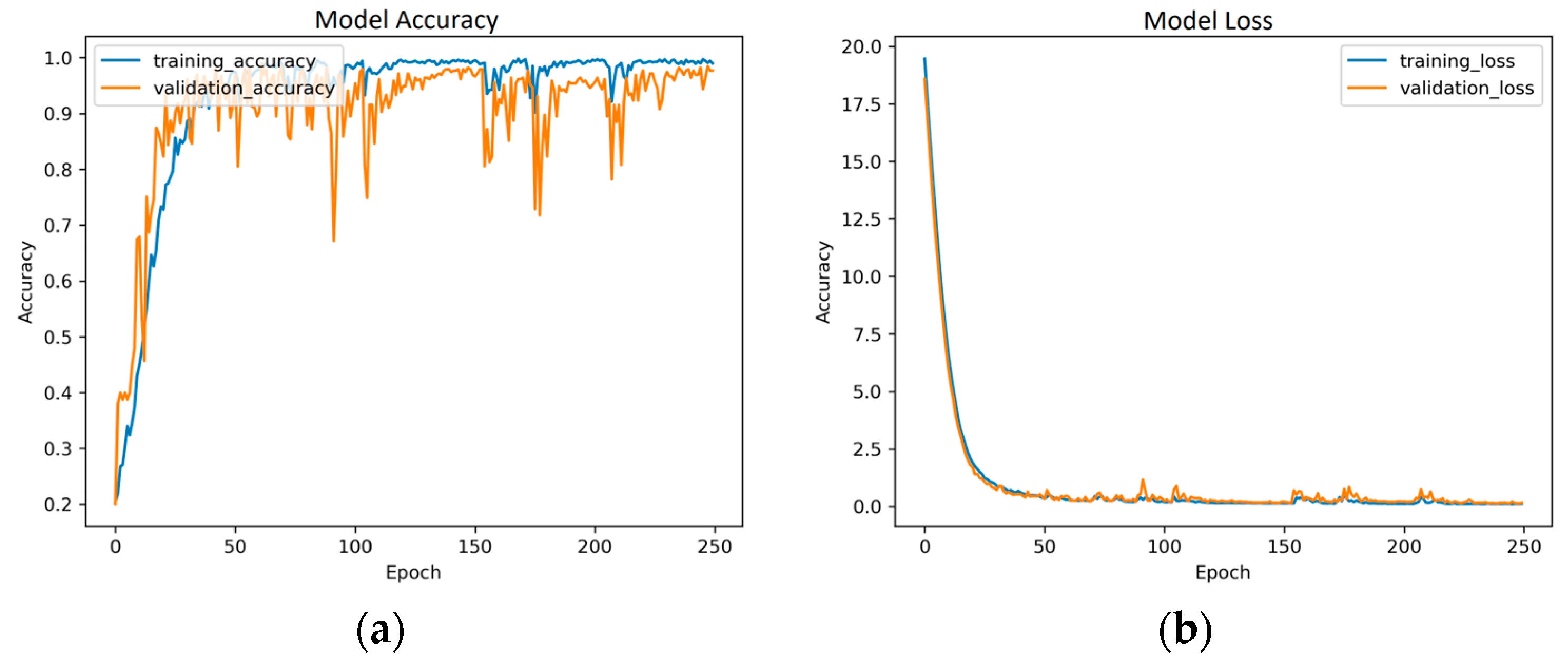
Figure 12.
Proposed model training history from cloth affected by airflow: (a) Model accuracy; (b) Model loss.
Table 6 presents the results of the classification performance of accuracy, precision, recall, and f1-score of the three methods. The results show that the transformer model achieved 99.01% accuracy, which was better than any of the other methods, and the precision, recall, and f1-score were higher than those of the LSTM and GRU models.
Table 6.
Classification Accuracy, Precision, Recall, and F1-Score comparison with Transformer, LSTM, and GRU models.
4.3. Discussion
In the previous studies in this area, researchers have presented various methods based on traditional machine learning techniques to accurately identify multiple garments in real-time, thus enhancing online virtual clothing style selection and benefiting the broader clothing industry.
Medina et al. [41] introduced a method employing CNN and VGG16 for cloth classification based on feature extraction, which achieved an accuracy of 90%. On the other hand, Chang et al. [42] utilized R-CNN with YOLOv5s for feature extraction and fabric classification, thus attaining the highest accuracy of 97%. However, both approaches encountered limitations due to the small size of their datasets, leading to a restricted number of images. Further, some types of cloth fell outside the camera’s capture area, resulting in an inability to accurately identify certain cloth objects. As presented in Table 7, the proposed approach combining ResNet50 for feature extraction with the Transformer model exhibited performance that was superior to that of any of the other methods. In our assessment, the deep learning model achieved enhanced accuracy in recognizing and classifying cloth simulations while significantly reducing the time for confusion compared to alternative models. This efficiency is attributed to the Transformer model’s parallel execution, which conserves device resources during execution.
Table 7.
Model comparison-table with state-of-the-art models.
The higher recognition and classification accuracy of the proposed model can be attributed to three main features: (i) Robustness to variations in physical properties, encompassing cloth color, the brightness of the cloth object in the video, random rotation angles of the video on the screen, and image resolution in the videos. (ii) Effective utilization of transfer learning techniques, enabling the model to be trained efficiently with a substantial amount of datasets. (iii) Efficient execution during the training process, thus obtaining significant time savings and a cost-effective solution. This is achieved through a fully automated end-to-end architecture for feature extraction and classification.
5. Conclusions
In this paper, we proposed a model for classifying clothes video scenes, specifically while focusing on clothes video summarization using DL techniques. Our proposed transformer model stands out in terms of performance, as it achieves excellent accuracy of 99.01%. This accuracy surpasses both state-of-the-art and recent research endeavors. Our evaluation encompasses a dataset of 1275 videos that have been meticulously categorized into five classes: solid cloth, very solid cloth, normal cloth, lightweight cloth, and very lightweight cloth.
In evaluating our proposed model, we also conducted a comparison with recently proposed models, specifically deep learning models such as CNN + VGG16 and R-CNN + YOLOv5s. This comparison provides a comprehensive performance evaluation, and the results demonstrate a remarkable improvement in terms of accuracy. Our focus lies in refining temporal frames analysis and minimizing preprocessing time, which has historically required seven to eight days to complete.
Our research trajectory also involves exploring novel models such as Recurrent Neural Networks (RNNs), Reinforcement Learning, Convolutional Neural Networks (CNNs), and pre-trained models including Inception V3, VGG16, VGG19, ResNet19, and EfficientNet. To enhance our approach, we also plan to analyze diverse datasets. This effort will not only validate our findings but also broaden the scope of our research.
Author Contributions
M.H. provided conceptualization, project administration, and edited and reviewed the manuscript. A.L. provided conceptualization and edited the manuscript. H.V. implemented the simulation and data curation. M.M. format analysis, methodology, software, preparing original draft, and writing—review and editing. All authors have read and agreed to the published version of the manuscript.
Funding
This research was supported by Basic Science Research Program through the National Research Foundation of Korea (NRF) funded by the Ministry of Education (NRF-2022R1I1A3069371), was funded by BK21 FOUR (Fostering Outstanding Universities for Research) (No.:5199990914048), and was supported by the Soonchunhyang University Research Fund.
Institutional Review Board Statement
Not applicable.
Informed Consent Statement
Not applicable.
Data Availability Statement
Not applicable.
Conflicts of Interest
The authors declare no conflict of interest.
References
- Krupiński, R. Simulation and Analysis of Floodlighting Based on 3D Computer Graphics. Energies 2021, 14, 1042. [Google Scholar] [CrossRef]
- Elshenawy, M.; Fahmy, A.; Elsamahy, A.; Kandil, S.A.; El Zoghby, H.M. Optimal Power Management of Interconnected Microgrids Using Virtual Inertia Control Technique. Energies 2022, 15, 7026. [Google Scholar] [CrossRef]
- Dehghani, M.; Montazeri, Z.; Dhiman, G.; Malik, O.P.; Morales-Menendez, R.; Ramirez-Mendoza, R.A.; Dehghani, A.; Guerrero, J.M.; Parra-Arroyo, L. A Spring Search Algorithm Applied to Engineering Optimization Problems. Appl. Sci. 2020, 10, 6173. [Google Scholar] [CrossRef]
- Hosseini, S.; Vázquez-Villegas, P.; Martínez-Chapa, S.O. Paper and Fiber-Based Bio-Diagnostic Platforms: Current Challenges and Future Needs. Appl. Sci. 2017, 7, 863. [Google Scholar] [CrossRef]
- Va, H.; Choi, M.-H.; Hong, M. Real-Time Cloth Simulation Using Compute Shader in Unity3D for AR/VR Contents. Appl. Sci. 2021, 11, 8255. [Google Scholar] [CrossRef]
- Escobar-Castillejos, D.; Noguez, J.; Cárdenas-Ovando, R.A.; Neri, L.; Gonzalez-Nucamendi, A.; Robledo-Rella, V. Using Game Engines for Visuo-Haptic Learning Simulations. Appl. Sci. 2020, 10, 4553. [Google Scholar] [CrossRef]
- Matsui, T.; Suzuki, K.; Sato, S.; Kubokawa, Y.; Nakamoto, D.; Davaakhishig, S.; Matsumoto, Y. Pilot Demonstration of a Strengthening Method for Steel-Bolted Connections Using Pre-Formable Carbon Fiber Cloth with VaRTM. Materials 2021, 14, 2184. [Google Scholar] [CrossRef]
- Kang, D.; Lee, T.; Shin, Y.; Seo, S. Video-based Stained Glass. KSII Trans. Internet Inf. Syst. 2022, 16, 2345–2358. [Google Scholar]
- Mangenda Tshiaba, S.; Wang, N.; Ashraf, S.F.; Nazir, M.; Syed, N. Measuring the Sustainable Entrepreneurial Performance of Textile-Based Small–Medium Enterprises: A Mediation–Moderation Model. Sustainability 2021, 13, 11050. [Google Scholar] [CrossRef]
- Junbang, L.; Lin, M.; Koltun, V. Differentiable cloth simulation for inverse problems. Adv. Neural Inf. Process. Syst. 8 Dec 2019, 32, 1–10. Available online: https://proceedings.neurips.cc/paper/2019/hash/28f0b864598a1291557bed248a998d4e-Abstract.html (accessed on 8 December 2019).
- Kumar, T.A.; Rekha, G. Challenges of Applying Deep Learning in Real-World Applications. Challenges and Applications for Implementing Machine Learning in Computer Vision; IGI Global: Hershey, PA, USA, 2020; pp. 92–118. [Google Scholar]
- Vilakone, P.; Park, D.-S. The Efficiency of a DoParallel Algorithm and an FCA Network Graph Applied to Recommendation System. Appl. Sci. 2020, 10, 2939. [Google Scholar] [CrossRef]
- Chen, X.W.; Lin, X. Big data deep learning: Challenges and perspectives. IEEE Access 2014, 2, 514–525. [Google Scholar] [CrossRef]
- Cetinel, H.; Öztürk, H.; Çelik, E.; Karlık, B. Artificial neural network-based prediction technique for wear loss quantities in Mo coatings. Wear 2006, 261, 1064–1068. [Google Scholar] [CrossRef]
- Lahner, Z.; Cremers, D.; Tung, T. Deepwrinkles: Accurate and realistic clothing modeling. In Proceedings of the European Conference on Computer Vision (ECCV), Munich, Germany, 8–14 September 2018; pp. 667–684. [Google Scholar]
- Ju, E.; Choi, M.G. Estimating Cloth Simulation Parameters from a Static Drape Using Neural Networks. IEEE Access 2020, 8, 195121. [Google Scholar] [CrossRef]
- Tae Min, L.; Jin Oh, Y.; Lee, I.-K. Efficient cloth simulation using miniature cloth and upscaling deep neural networks. arXiv 2019, arXiv:1907.03953. [Google Scholar]
- Bertiche, H.; Madadi, M.; Escalera, S. Neural Cloth Simulation. ACM Trans. Graph. 2022, 41, 1–14. [Google Scholar] [CrossRef]
- Artur, G.; Black, M.J.; Hilliges, O. HOOD: Hierarchical Graphs for Generalized Modelling of Clothing Dynamics. In Proceedings of the IEEE/CVF Conference on Computer Vision and Pattern Recognition, Vancouver Convention Center, Vancouver, BC, Canada, 18–22 June 2023. [Google Scholar]
- Andrade, J.E.; Tu, X. Multiscale framework for behavior prediction in granular media. Mech. Mater. 2009, 41, 652–669. [Google Scholar] [CrossRef]
- Dixit, A.; Mali, S.H. Modeling techniques for predicting the mechanical properties of woven-fabric textile composites: A review. Mech. Compos. Mater. 2013, 49, 1–20. [Google Scholar] [CrossRef]
- Liao, K.; Fan, B.; Zheng, Y.; Lin, G.; Cao, C. Image Retrieval Based on the Weighted and Regional Integration of CNN Features. KSII Trans. Internet Inf. Syst. 2022, 16, 894–907. [Google Scholar]
- Lecun, Y.; Bottou, L.; Bengio, Y.; Haffner, P. Gradient-based learning applied to document recognition. Proc. IEEE 1998, 86, 2278–2324. [Google Scholar] [CrossRef]
- Krizhevsky, A.; Sutskever, I.; Hinton, E.G. ImageNet classification with deep convolutional neural networks. Commun. ACM 2017, 60, 84–90. [Google Scholar] [CrossRef]
- Zhang, K.; Guo, Y.; Wang, X.; Yuan, J.; Ding, Q. Multiple Feature Reweight DenseNet for Image Classification. IEEE Access 2019, 7, 9872–9880. [Google Scholar] [CrossRef]
- Sarwinda, D.; Paradisa, H.R.; Bustamam, A.; Anggia, P. Deep learning in image classification using residual network (ResNet) variants for detection of colorectal cancer. Procedia Comput. Sci. 2021, 179, 423–431. [Google Scholar] [CrossRef]
- Wang, C.; Chen, D.; Hao, L.; Liu, X.; Zeng, Y.; Chen, J.; Zhang, G. Pulmonary image classification based on inception-v3 transfer learning model. IEEE Access 2019, 7, 146533–146541. [Google Scholar] [CrossRef]
- Wan-Duo Kurt, M.; Lewis, J.P.; Bastiaan Kleijn, W. The HSIC bottleneck: Deep learning without back-propagation. In Proceedings of the AAAI Conference on Artificial Intelligence, New York, NY, USA, 7–12 February 2020; Volume 34, p. 4. [Google Scholar]
- Rothman, D.; Gulli, A. Transformers for Natural Language Processing: Build, Train, and Fine-Tune Deep Neural Network Architectures for NLP with Python, PyTorch, TensorFlow, BERT, and GPT-3; Packt Publishing Ltd.: Birmingham, UK, 2022. [Google Scholar]
- Zhao, H.; Jiang, L.; Jia, J.; Torr, P.H.S.; Koltun, V. Point transformer. In Proceedings of the IEEE/CVF International Conference on Computer Vision, Montreal, BC, Canada, 11–17 October 2021; pp. 16259–16268. [Google Scholar]
- Dosovitskiy, A.; Beyer, L.; Kolesnikov, A.; Weissenborn, D.; Zhai, X.; Unterthiner, T.; Dehghani, M.; Minderer, M.; Heigold, G.; Gelly, S.; et al. An image is worth 16 × 16 words: Transformers for image recognition at scale. arXiv 2021, arXiv:2010.11929. [Google Scholar]
- Dong, L.; Shuang, X.; Xu, B. Speech-transformer: A no-recurrence sequence-to-sequence model for speech recognition. In Proceedings of the IEEE International Conference on Acoustics, Speech and Signal Processing (ICASSP), Calgary, AB, Canada, 15–20 April 2018; IEEE: New York, NY, USA, 2018. [Google Scholar]
- Chen, L.; Lu, K.; Rajeswaran, A.; Lee, K.; Grover, A.; Laskin, M.; Abbeel, P.; Srinivas, A.; Mordatch, I. Decision transformer: Reinforcement learning via sequence modeling. Adv. Neural Inf. Process. Syst. 2021, 34, 15084–15097. [Google Scholar]
- Meng, Y.; Yuan, D.; Su, S.; Ming, Y. A Novel Transfer Learning-Based Algorithm for Detecting Violence Images. KSII Trans. Internet Inf. Syst. 2022, 16, 1818–1832. [Google Scholar]
- Gao, G.; Xu, Z.; Li, J.; Yang, J.; Zeng, T.; Qi, G.-J. CTCNet: A CNN-Transformer Cooperation Network for Face Image Super-Resolution. IEEE Trans. Image Process. 2023, 32, 1978–1991. [Google Scholar] [CrossRef]
- ur Rehman, A.; Belhaouari, S.B.; Kabir, M.A.; Khan, A. On the Use of Deep Learning for Video Classification. Appl. Sci. 2023, 13, 2007. [Google Scholar] [CrossRef]
- Sarma, M.S.; Deb, K.; Dhar, P.K.; Koshiba, T. Traditional Bangladeshi Sports Video Classification Using Deep Learning Method. Appl. Sci. 2021, 11, 2149. [Google Scholar] [CrossRef]
- Reinolds, F.; Neto, C.; Machado, J. Deep Learning for Activity Recognition Using Audio and Video. Electronics 2022, 11, 782. [Google Scholar] [CrossRef]
- Vrskova, R.; Kamencay, P.; Hudec, R.; Sykora, P. A New Deep-Learning Method for Human Activity Recognition. Sensors 2023, 23, 2816. [Google Scholar] [CrossRef] [PubMed]
- Shan, Y.; Liang, J.; Ming, C.L. Learning-based cloth material recovery from video. In Proceedings of the IEEE International Conference on Computer Vision, Venice, Italy, 22–29 October 2017; pp. 4383–4393. [Google Scholar]
- Medina, A.; Méndez, J.I.; Ponce, P.; Peffer, T.; Meier, A.; Molina, A. Using Deep Learning in Real-Time for Clothing Classification with Connected Thermostats. Energies 2022, 15, 1811. [Google Scholar] [CrossRef]
- Chang, Y.-H.; Zhang, Y.-Y. Deep Learning for Clothing Style Recognition Using YOLOv5. Micromachines 2022, 13, 1678. [Google Scholar] [CrossRef]


Disclaimer/Publisher’s Note: The statements, opinions and data contained in all publications are solely those of the individual author(s) and contributor(s) and not of MDPI and/or the editor(s). MDPI and/or the editor(s) disclaim responsibility for any injury to people or property resulting from any ideas, methods, instructions or products referred to in the content. |
© 2023 by the authors. Licensee MDPI, Basel, Switzerland. This article is an open access article distributed under the terms and conditions of the Creative Commons Attribution (CC BY) license (https://creativecommons.org/licenses/by/4.0/).