

Modeling of Traffic Flows Sustainability on Highway Network Stretches


 ,
,  and
and 
Abstract
:1. Introduction
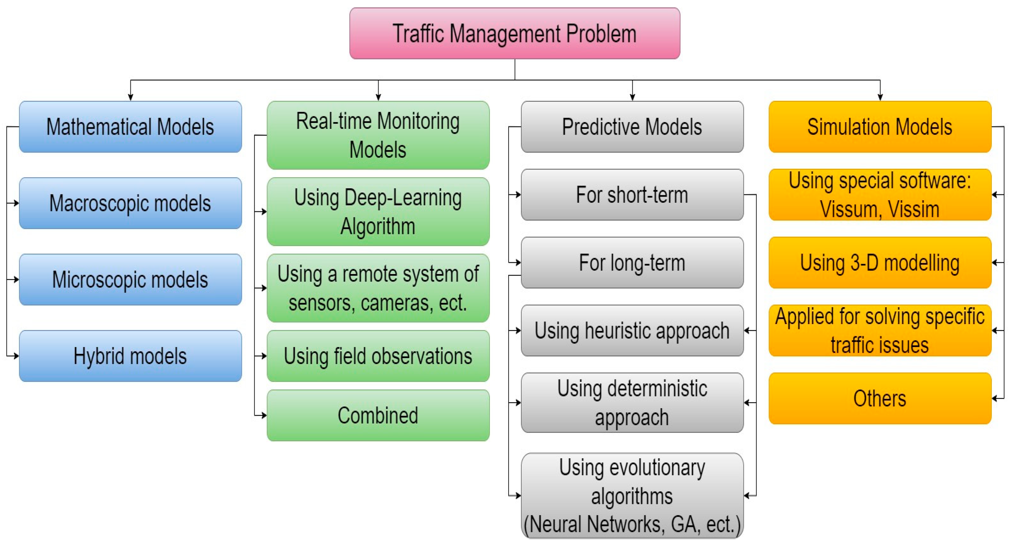
1.1. General Models for Solving the Real-Time Traffic Management Problem and Predicting Traffic Flows
1.2. Macroscopic Models of the Traffic Flows
1.3. Microscopic Models of the Traffic Flows
1.4. Hybrid Models of the Traffic Flows
1.5. Knowledge Gap Identification and Research Novelty
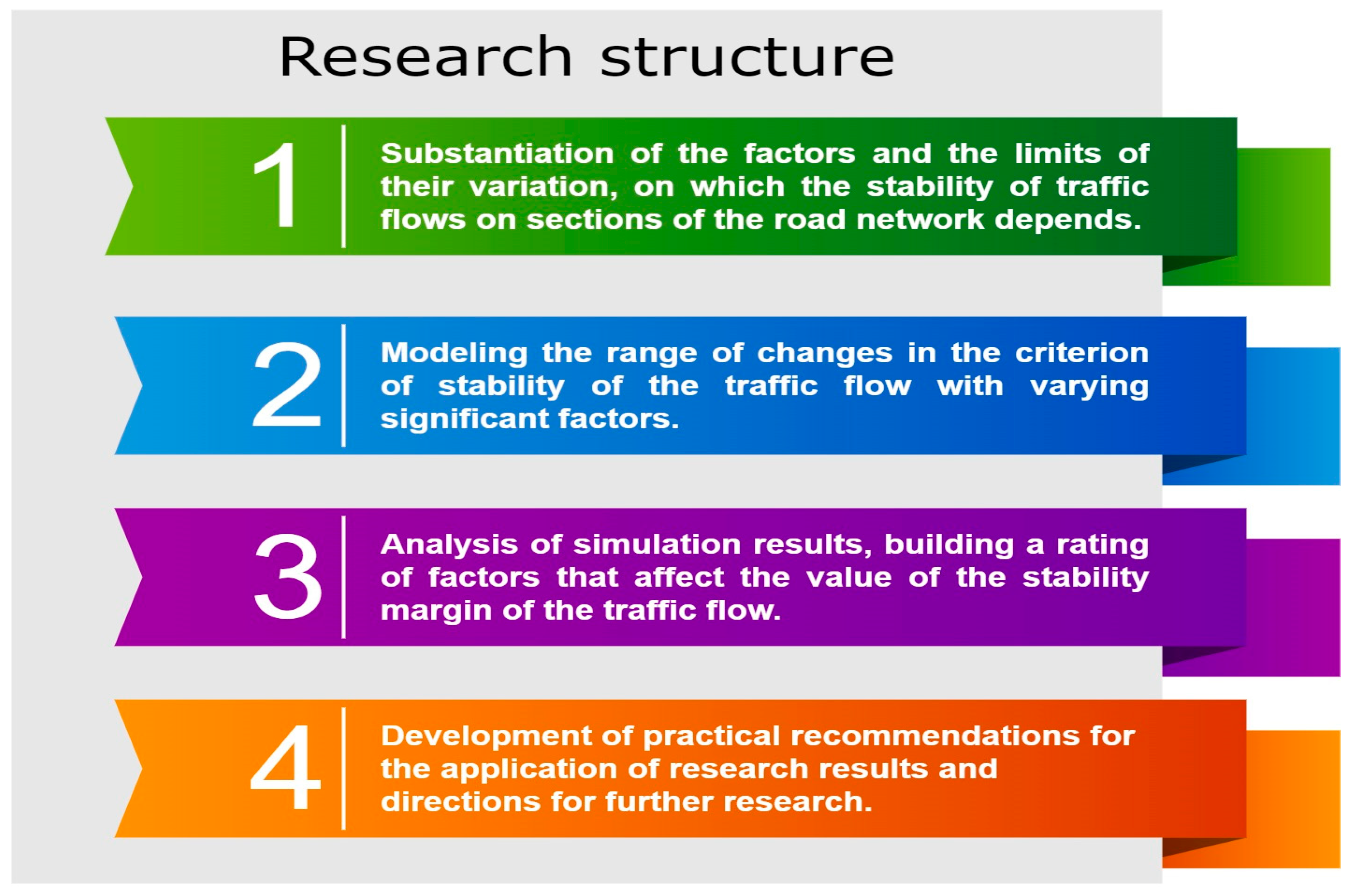
1.6. Conceptualization of Current Research Framework and Study Objective
1.7. Purpose and Objectives of the Study
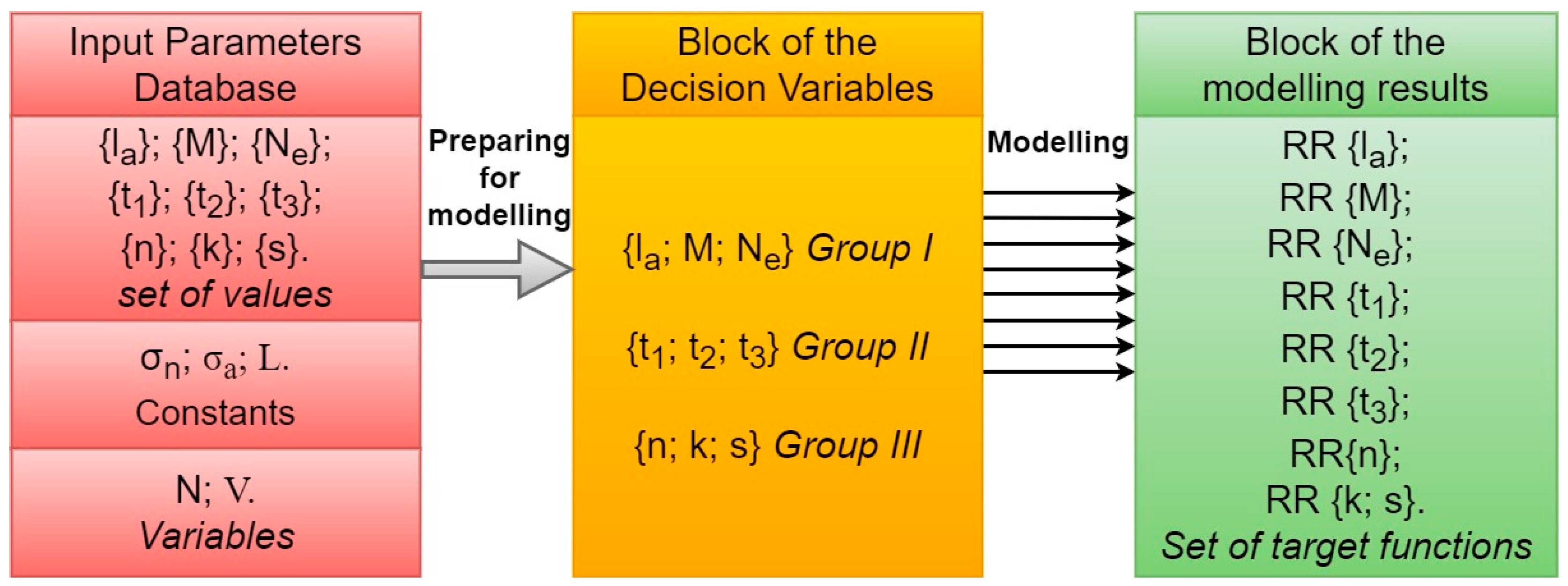
2. Materials and Methods
3. Results
4. Discussion
- −
- The study of factors that impact traffic flow sustainability was only conducted in the values range presented in Table 1;
- −
- robustness criterion assessment was only applied for a highway stretch with a fixed length equal to one kilometer;
- −
- the group of factors characterizing weather conditions was not considered when determining the dependencies of factors that impact the target function RR;
- −
- the robustness criterion is only applicable to evaluating traffic flow sustainability on a particular highway section and cannot be used to assess the entire urban transport network;
- −
- RR did not directly consider the vehicle intensity, although the traffic flow density and speed gradients were used among the estimated factors.
- −
- We hope these limitations do not reduce the scientific and practical significance of the proposed approach.
5. Conclusions
Author Contributions
Funding
Institutional Review Board Statement
Informed Consent Statement
Data Availability Statement
Acknowledgments
Conflicts of Interest
References
- Kessels, F. Introduction to Traffic Flow Modelling. In Traffic Flow Modelling. EURO Advanced Tutorials on Operational Research; Springer: Cham, Switzerland, 2019; pp. 1–19. [Google Scholar] [CrossRef]
- Johari, M.; Keyvan-Ekbatani, M.; Leclercq, L.; Ngoduy, D.; Mahmassani, H.S. Macroscopic network-level traffic models: Bridging fifty years of development toward the next era. Transp. Res. Part C Emerg. Technol. 2021, 131, 103334. [Google Scholar] [CrossRef]
- Trojanowski, P.; Trusz, A.; Stupin, B. Correlation Between Accidents on Selected Roads as Fundamental for Determining the Safety Level of Road Infrastructure. In Advances in Design, Simulation and Manufacturing V, Proceedings of the 5th International Conference on Design, Simulation, Manufacturing: The Innovation Exchange, DSMIE-2022, Poznan, Poland, 7–10 June 2022; Lecture Notes in Mechanical Engineering; Ivanov, V., Trojanowska, J., Pavlenko, I., Rauch, E., Peraković, D., Eds.; Springer: Cham, Switzerland, 2022; pp. 104–113. [Google Scholar] [CrossRef]
- Nagatani, T. Macroscopic traffic flow in multiple-loop networks. Phys. A Stat. Mech. Appl. 2023, 609, 128324. [Google Scholar] [CrossRef]
- Herty, M.; Kolbe, N. Data-Driven Models for Traffic Flow at Junctions. arXiv 2022, arXiv:2212.08912. [Google Scholar] [CrossRef]
- Karafyllis, I.; Theodosis, D.; Papageorgiou, M. Stability analysis of nonlinear inviscid microscopic and macroscopic traffic flow models of bidirectional cruise-controlled vehicles. IMA J. Math. Control Inf. 2022, 39, 609–642. [Google Scholar] [CrossRef]
- Pompigna, A.; Mauro, R. A Statistical Simulation Model for the Analysis of the Traffic Flow Reliability and the Probabilistic Assessment of the Circulation Quality on a Freeway Segment. Sustainability 2022, 14, 16019. [Google Scholar] [CrossRef]
- González-Gómez, K.; Rollins, D.K.; Castro, M. Modeling Urban Road Scenarios to Evaluate Intersection Visibility. Sustainability 2022, 14, 354. [Google Scholar] [CrossRef]
- Volkov, V.; Taran, I.; Volkova, T.; Pavlenko, O.; Berezhnaja, N. Determining the Efficient Management System for a Specialized Transport Enterprise. Nauk. Visnyk Natsionalnoho Hirnychoho Universytetu 2020, 4, 185–191. [Google Scholar] [CrossRef]
- Muzylyov, D.; Shramenko, N. Mathematical Model of Reverse Loading Advisability for Trucks Considering Idle Times. In New Technologies, Development and Application III. NT 2020; Lecture Notes in Networks and Systems; Karabegović, I., Ed.; Springer: Cham, Switzerland, 2020; Volume 128, pp. 612–620. [Google Scholar] [CrossRef]
- Calsavara, F.; Kabbach, F.I., Jr.; Larocca, A.P.C. Effects of Fog in a Brazilian Road Segment Analyzed by a Driving Simulator for Sustainable Transport: Drivers’ Speed Profile under In-Vehicle Warning Systems. Sustainability 2021, 13, 10501. [Google Scholar] [CrossRef]
- Calsavara, F.; Kabbach, F.I., Jr.; Larocca, A.P.C. Effects of Fog in a Brazilian Road Segment Analyzed by a Driving Simulator for Sustainable Transport: Drivers’ Visual Profile. Sustainability 2021, 13, 9448. [Google Scholar] [CrossRef]
- Kolosz, B.; Grant-Muller, S. Comparing smart scheme effects for congested highways. Transp. Res. Part C Emerg. Technol. 2015, 60, 313–323. [Google Scholar] [CrossRef]
- Sharma, A.; Sharma, A.; Nikashina, P.; Gavrilenko, V.; Tselykh, A.; Bozhenyuk, A.; Masud, M.; Meshref, H. A Graph Neural Network (GNN)-Based Approach for Real-Time Estimation of Traffic Speed in Sustainable Smart Cities. Sustainability 2023, 15, 11893. [Google Scholar] [CrossRef]
- Zeng, W.; Wang, K.; Zhou, J.; Cheng, R. Traffic Flow Prediction Based on Hybrid Deep Learning Models Considering Missing Data and Multiple Factors. Sustainability 2023, 15, 11092. [Google Scholar] [CrossRef]
- Guo, C.; Li, D.; Chen, X. Unequal Interval Dynamic Traffic Flow Prediction with Singular Point Detection. Appl. Sci. 2023, 13, 8973. [Google Scholar] [CrossRef]
- Li, L.; Ji, X.; Gan, J.; Qu, X.; Ran, B. A macroscopic model of heterogeneous traffic flow based on the safety potential field theory. IEEE Access 2021, 9, 7460–7470. [Google Scholar] [CrossRef]
- Imran, W.; Khan, Z.H.; Gulliver, T.A.; Khattak, K.S.; Nasir, H. A macroscopic traffic model for heterogeneous flow. Chin. J. Phys. 2020, 63, 419–435. [Google Scholar] [CrossRef]
- Khan, Z.H.; Gulliver, T.A.; Imran, W.; Khattak, K.S.; Altamimi, A.B.; Qazi, A. A macroscopic traffic model based on relaxation time. Alex. Eng. J. 2022, 61, 585–596. [Google Scholar] [CrossRef]
- Briani, M.; Cristiani, E.; Onofri, E. Inverting the Fundamental Diagram and Forecasting Boundary Conditions: How Machine Learning Can Improve Macroscopic Models for Traffic Flow. arXiv 2023, arXiv:2303.12740. [Google Scholar] [CrossRef]
- Bouadi, M.; Jia, B.; Jiang, R.; Li, X.; Gao, Z.Y. Traffic flow stability in stochastic second-order macroscopic continuum model. arXiv 2022, arXiv:2204.13937. [Google Scholar] [CrossRef]
- Xue, Y.; Zhang, Y.; Fan, D.; Zhang, P.; He, H.D. An extended macroscopic model for traffic flow on curved road and its numerical simulation. Nonlinear Dyn. 2019, 95, 3295–3307. [Google Scholar] [CrossRef]
- Wang, Y.; Yu, X.; Guo, J.; Papamichail, I.; Papageorgiou, M.; Zhang, L.; Sun, J. Macroscopic traffic flow modelling of large-scale freeway networks with field data verification: State-of-the-art review, benchmarking framework, and case studies using METANET. Transp. Res. Part C Emerg. Technol. 2022, 145, 103904. [Google Scholar] [CrossRef]
- Liu, H.; Claudel, C.G.; Machemehl, R.; Perrine, K.A. A Robust Traffic Control Model Considering Uncertainties in Turning Ratios. IEEE Trans. Intell. Transp. Syst. 2022, 23, 6539–6555. [Google Scholar] [CrossRef]
- Yan, H.; Fu, L.; Qi, Y.; Yu, D.-J.; Ye, Q. Robust ensemble method for short-term traffic flow prediction. Future Gener. Comput. Syst. 2022, 133, 395–410. [Google Scholar] [CrossRef]
- Zheng, Q.; Feng, X.; Zheng, H. Robust Prediction of Traffic Flow Based on Multi-Task Graph Convolution Network. In Proceedings of the 2020 IEEE 6th International Conference on Computer and Communications (ICCC), Chengdu, China, 11–14 December 2020; pp. 2053–2058. [Google Scholar] [CrossRef]
- Moussa, G.S.; Hussain, K.F. Robust Deep Learning Architecture for Traffic Flow Estimation from a Subset of Link Sensors. J. Transp. Eng. Part A Syst. 2020, 146, 04019055. [Google Scholar] [CrossRef]
- Alhariqi, A.; Gu, Z.; Saberi, M. Calibration of the intelligent driver model (IDM) with adaptive parameters for mixed autonomy traffic using experimental trajectory data. Transp. B Transp. Dyn. 2022, 10, 421–440. [Google Scholar] [CrossRef]
- Hajidavalloo, M.R.; Li, Z.; Chen, D.; Louati, A.; Feng, S.; Qin, W.B. Mechanical System Inspired Microscopic Traffic Model: Modeling, Analysis, and Validation. IEEE Trans. Intell. Veh. 2022, 8, 301–312. [Google Scholar] [CrossRef]
- Yuan, T.; Alasiri, F.; Ioannou, P.A. Selection of the speed command distance for improved performance of a rule-based vsl and lane change control. IEEE Trans. Intell. Transp. Syst. 2022, 23, 19348–19357. [Google Scholar] [CrossRef]
- Yuan, C.; Li, Y.; Huang, H.; Wang, S.; Sun, Z.; Li, Y. Using traffic flow characteristics to predict real-time conflict risk: A novel method for trajectory data analysis. Anal. Methods Accid. Res. 2022, 35, 100217. [Google Scholar] [CrossRef]
- Das, A.; Ahmed, M.M. Adjustment of key lane change parameters to develop microsimulation models for representative assessment of safety and operational impacts of adverse weather using SHRP2 naturalistic driving data. J. Saf. Res. 2022, 81, 9–20. [Google Scholar] [CrossRef]
- Lazar, H. Comparison of microscopic car following models. In Proceedings of the 2019 International Conference on Systems of Collaboration Big Data, Internet of Things & Security (SysCoBIoTS), Casablanca, Morocco, 12–13 December 2019; IEEE: Piscataway, NJ, USA, 2019; pp. 1–6. [Google Scholar] [CrossRef]
- Feng, T.; Liu, K.; Liang, C. An Improved Cellular Automata Traffic Flow Model Considering Driving Styles. Sustainability 2023, 15, 952. [Google Scholar] [CrossRef]
- Zhao, J.; Knoop, V.L.; Wang, M. Microscopic traffic modeling inside intersections: Interactions between drivers. Transp. Sci. 2023, 57, 135–155. [Google Scholar] [CrossRef]
- Zhao, J.; Knoop, V.L.; Wang, M. Two-dimensional vehicular movement modelling at intersections based on optimal control. Transp. Res. Part B Methodol. 2020, 138, 1–22. [Google Scholar] [CrossRef]
- Bieletska, O.; Liubyi, Y.; Ocheretenko, S.; Muzylyov, D.; Ivanov, V.; Pavlenko, I. Approach to Determine Transport Delays at Unsignalized Intersections. Commun. Sci. Lett. Univ. Zilina 2023, 25, 124–136. [Google Scholar] [CrossRef]
- Sakno, O.; Moisia, D.; Medvediev, I.; Kolesnikova, T.; Rogovyi, A. Development of the Software for the Road-Train Stable Movement Mode Research. In Advances in Intelligent Systems and Computing V, Proceedings of the CSIT 2020, Zbarazh, Ukraine, 23–26 September 2020; Advances in Intelligent Systems and Computing; Shakhovska, N., Medykovskyy, M.O., Eds.; Springer: Cham, Switzerland, 2021; Volume 1293, pp. 522–539. [Google Scholar] [CrossRef]
- Sakno, O.; Moisia, D.; Medvediev, I.; Kolesnikova, T.; Rogovyi, A. Linear and Non-linear Hheel Slip Hypothesis in Studying Stationary Modes of a Double Road Train. In Proceedings of the 2020 IEEE 15th International Conference on Computer Sciences and Information Technologies (CSIT), Zbarazh, Ukraine, 23–26 September 2020; pp. 183–187. [Google Scholar] [CrossRef]
- Kušić, K.; Schumann, R.; Ivanjko, E. A digital twin in transportation: Real-time synergy of traffic data streams and simulation for virtualizing motorway dynamics. Adv. Eng. Inform. 2023, 55, 101858. [Google Scholar] [CrossRef]
- Shang, X.C.; Liu, F.; Li, X.G.; Janssens, D.; Wets, G. The Impact of Three Specific Collaborative Merging Strategies on Traffic Flow. J. Adv. Transp. 2023, 2023, 1375867. [Google Scholar] [CrossRef]
- Bakibillah, A.S.M.; Hwa Tan, Y.; Yong Loo, J.; Pin Tan, C.; Kamal, M.A.S.; Pu, Z. Robust estimation of traffic density with missing data using an adaptive-R extended Kalman filter. Appl. Math. Comput. 2022, 421, 126915. [Google Scholar] [CrossRef]
- Wei, Z.; Peng, T.; Wei, S. A Robust Adaptive Traffic Signal Control Algorithm Using Q-Learning under Mixed Traffic Flow. Sustainability 2022, 14, 5751. [Google Scholar] [CrossRef]
- Zheng, G.; Chai, W.K.; Duanmu, J.L.; Katos, V. Hybrid deep learning models for traffic prediction in large-scale road networks. Inf. Fusion 2023, 92, 93–114. [Google Scholar] [CrossRef]
- Li, Z.; Wang, X.; Yang, K. An Effective Self-Attention-Based Hybrid Model for Short-Term Traffic Flow Prediction. Adv. Civ. Eng. 2023, 2023, 9308576. [Google Scholar] [CrossRef]
- Wen, J.; Hong, L.; Dai, M.; Xiao, X.; Wu, C. A stochastic model for stop-and-go phenomenon in traffic oscillation: On the prospective of macro and micro traffic flow. Appl. Math. Comput. 2023, 440, 127637. [Google Scholar] [CrossRef]
- Mittal, U.; Chawla, P.; Tiwari, R. EnsembleNet: A hybrid approach for vehicle detection and estimation of traffic density based on faster R-CNN and YOLO models. Neural Comput. Appl. 2023, 35, 4755–4774. [Google Scholar] [CrossRef]
- Djenouri, Y.; Belhadi, A.; Srivastava, G.; Lin, J.C.W. Hybrid graph convolution neural network and branch-and-bound optimization for traffic flow forecasting. Future Gener. Comput. Syst. 2023, 139, 100–108. [Google Scholar] [CrossRef]
- Xu, X.; Jin, X.; Xiao, D.; Ma, C.; Wong, S.C. A hybrid autoregressive fractionally integrated moving average and nonlinear autoregressive neural network model for short-term traffic flow prediction. J. Intell. Transp. Syst. 2023, 27, 1–18. [Google Scholar] [CrossRef]
- Novinkina, J.; Davydovitch, A.; Vasiljeva, T.; Haidabrus, B. Industries Pioneering Blockchain Technology for Electronic Data Interchange. Acta Logist. 2021, 8, 319–327. [Google Scholar] [CrossRef]
- Haidabrus, B.; Grabis, J.; Protsenko, S. Agile Project Management Based on Data Analysis for Information Management Systems. In Advances in Design, Simulation and Manufacturing IV, Proceedings of the 4th International Conference on Design, Simulation, Manufacturing: The Innovation Exchange, DSMIE-2021, Lviv, Ukraine, 8–11 June 2021; Lecture Notes in Mechanical Engineering; Ivanov, V., Trojanowska, J., Pavlenko, I., Zajac, J., Peraković, D., Eds.; Springer: Cham, Switzerland, 2021; pp. 174–182. [Google Scholar] [CrossRef]
- Sęk, J.; Trojanowski, P.; Gilewicz, Ł.; Gapinski, B.; Evtuhov, A. Implementation of Intelligent Transport Systems in an Urban Agglomeration: A Case Study. In Advances in Design, Simulation and Manufacturing VI, Proceedings of the 6th International Conference on Design, Simulation, Manufacturing: The Innovation Exchange, DSMIE-2023, High Tatras, Slovak Republic, 6–9 June 2023; Lecture Notes in Mechanical Engineering; Ivanov, V., Trojanowska, J., Pavlenko, I., Rauch, E., Piteľ, J., Eds.; Springer: Cham, Switzerland, 2023; pp. 152–161. [Google Scholar] [CrossRef]
- Zhu, Y.; Wu, Q.; Xiao, N. Research on highway traffic flow prediction model and decision-making method. Sci. Rep. 2022, 12, 19919. [Google Scholar] [CrossRef] [PubMed]
- Yang, H.; Du, L.; Zhang, G.; Ma, T. A Traffic Flow Dependency and Dynamics based Deep Learning Aided Approach for Network-Wide Traffic Speed Propagation Prediction. Transp. Res. Part B Methodol. 2023, 167, 99–117. [Google Scholar] [CrossRef]
- Ma, X.-X.; Xu, Y.-D. Robust Multi-Criteria Traffic Network Equilibrium Problems with Path Capacity Constraints. Axioms 2023, 12, 662. [Google Scholar] [CrossRef]
- Vojtov, V.A.; Muzylyov, D.O.; Karnaukh, M.V.; Kozenok, A.S.; Babych, I.A. Mathematical model of the traffic flow stability on a section of the road network in case of traffic jams. Cent. Ukr. Sci. Bull. Tech. Sci. 2023, 4, 24–33. [Google Scholar]
- Muzylyov, D.; Shramenko, N.; Karnaukh, M. Choice of Carrier Behavior Strategy According to Industry 4.0. In Advances in Design, Simulation and Manufacturing IV, DSMIE 2021; Lecture Notes in Mechanical Engineering; Ivanov, V., Trojanowska, J., Pavlenko, I., Zajac, J., Peraković, D., Eds.; Springer: Cham, Switzerland, 2021. [Google Scholar] [CrossRef]


| Parameter for Modeling | Label | Value | ||
|---|---|---|---|---|
| Minimal | Average | Maximal | ||
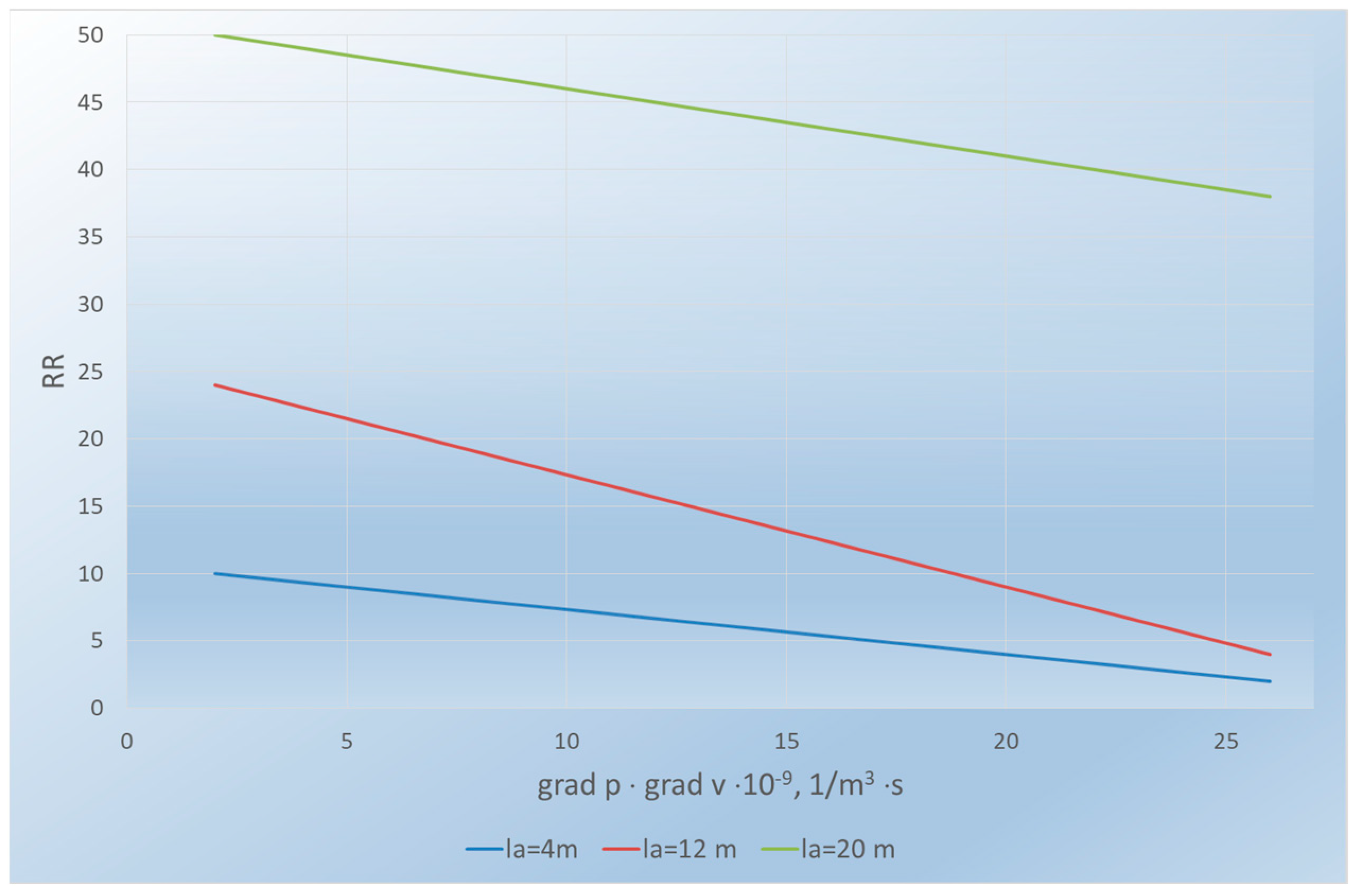
| Vehicle Length, m | la | 4 | 12 | 20 |
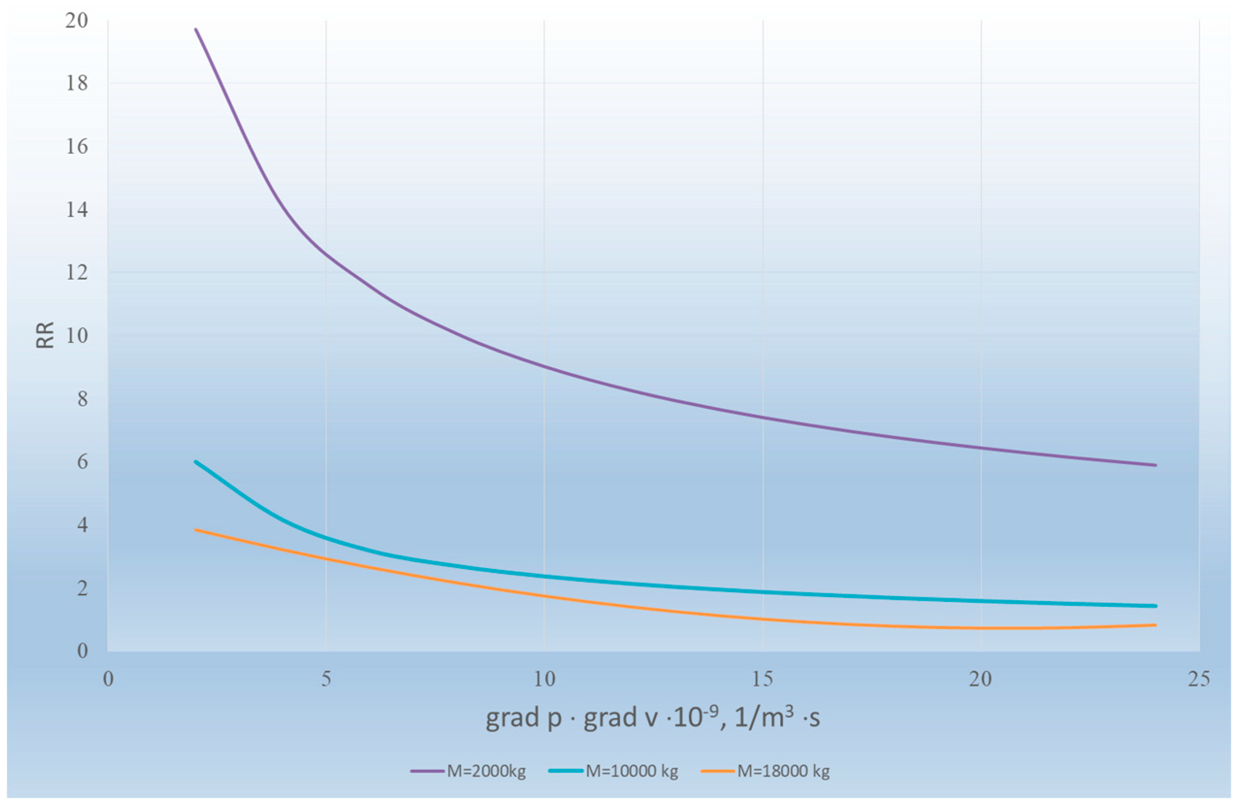
| Vehicle weight, kg | M | 2000 | 10,000 | 18,000 |
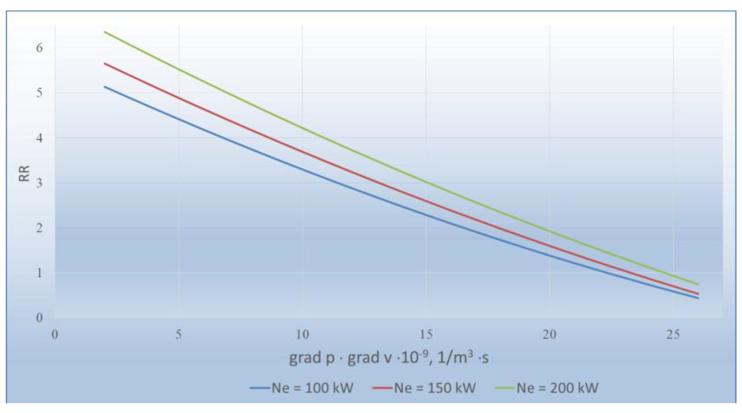
| Vehicle engine power, kW | Ne | 100 | 150 | 200 |
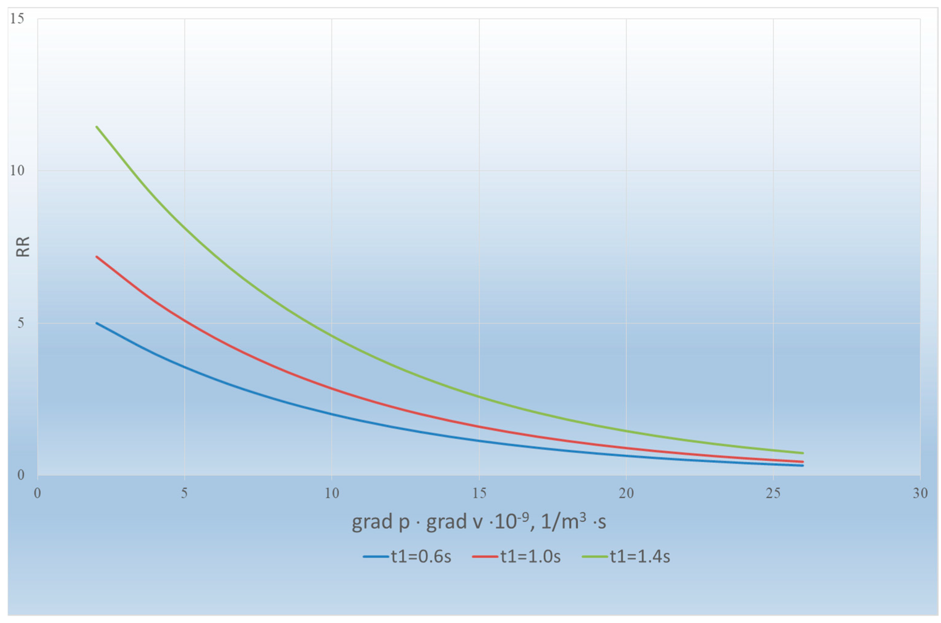
| Driver’s reaction time to the traffic situation, s | t1 | 0.6 | 1.0 | 1.4 |
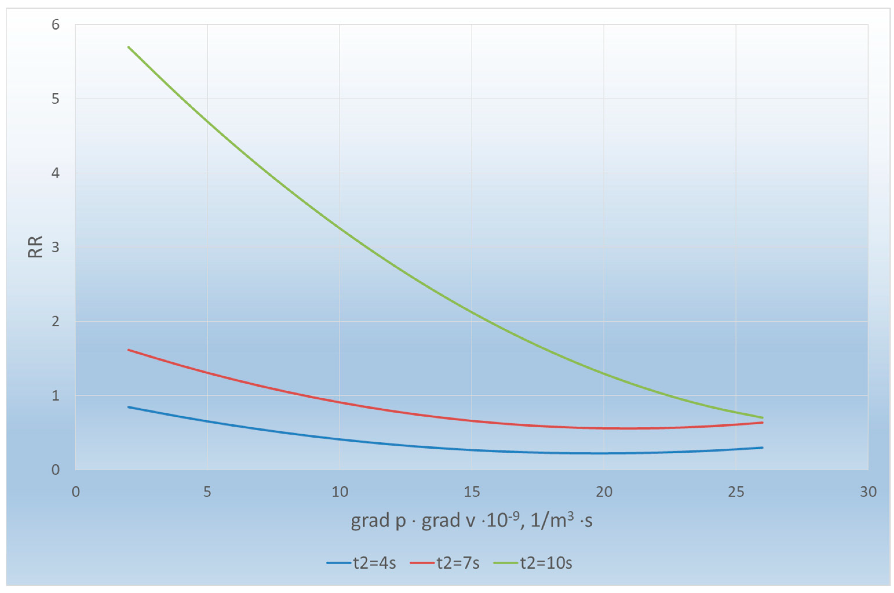
| Vehicle maneuver time according to traffic situation changes, s | t2 | 4 | 7 | 10 |
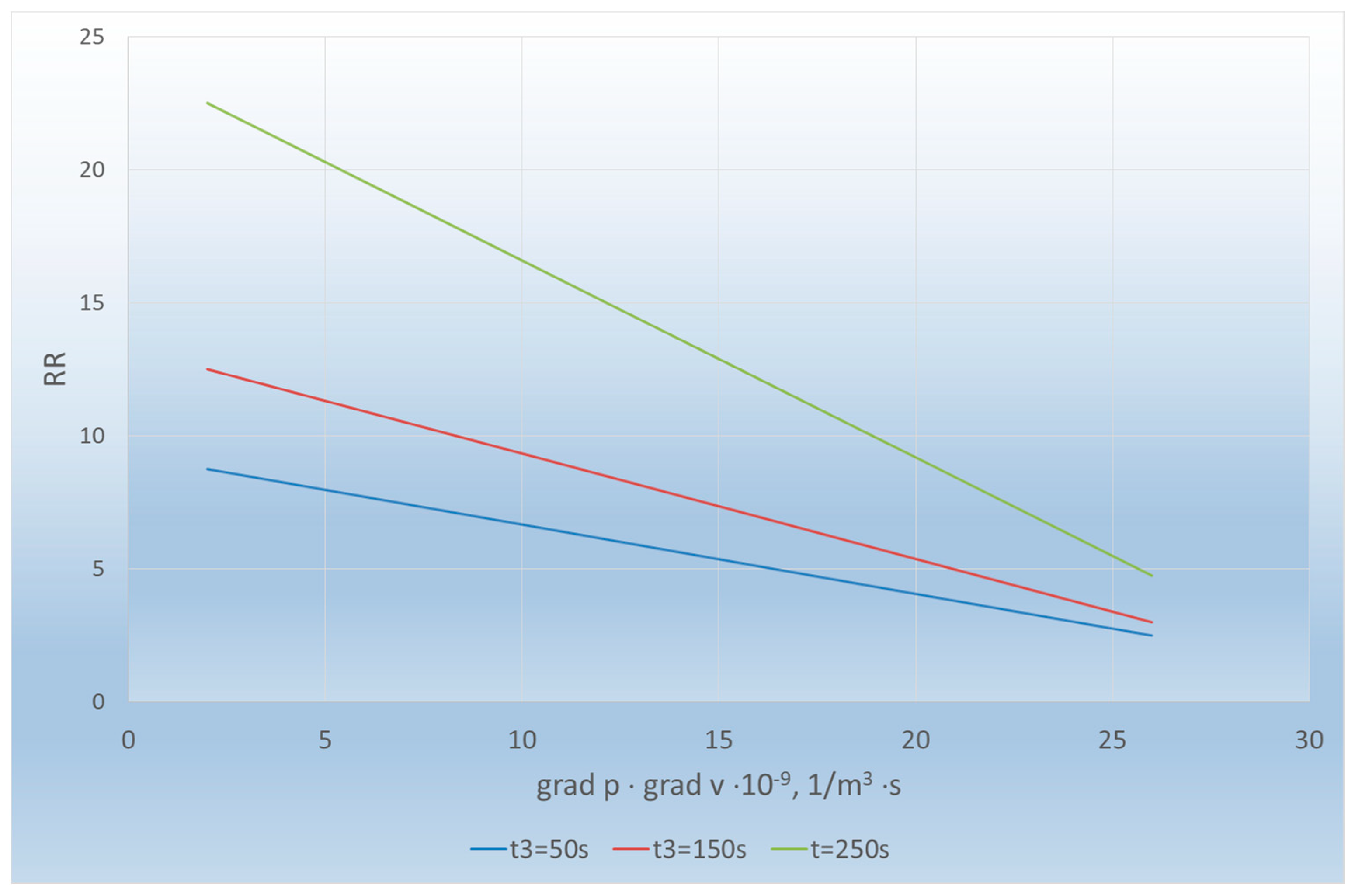
| Total delays time driving route, s | t3 | 50 | 150 | 250 |
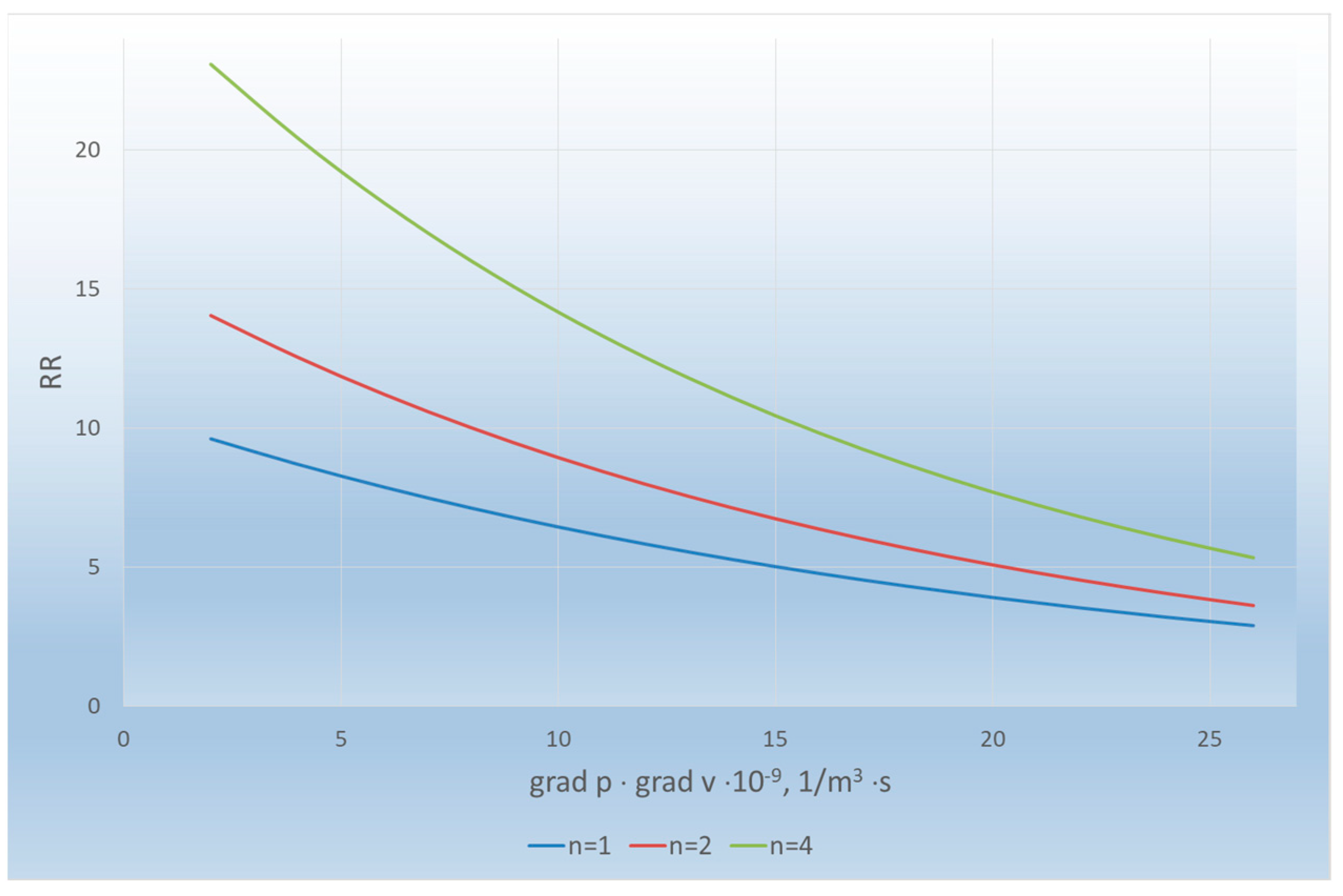
| Lanes quantity on the roadway, unit | n | 1 | 2 | 4 |
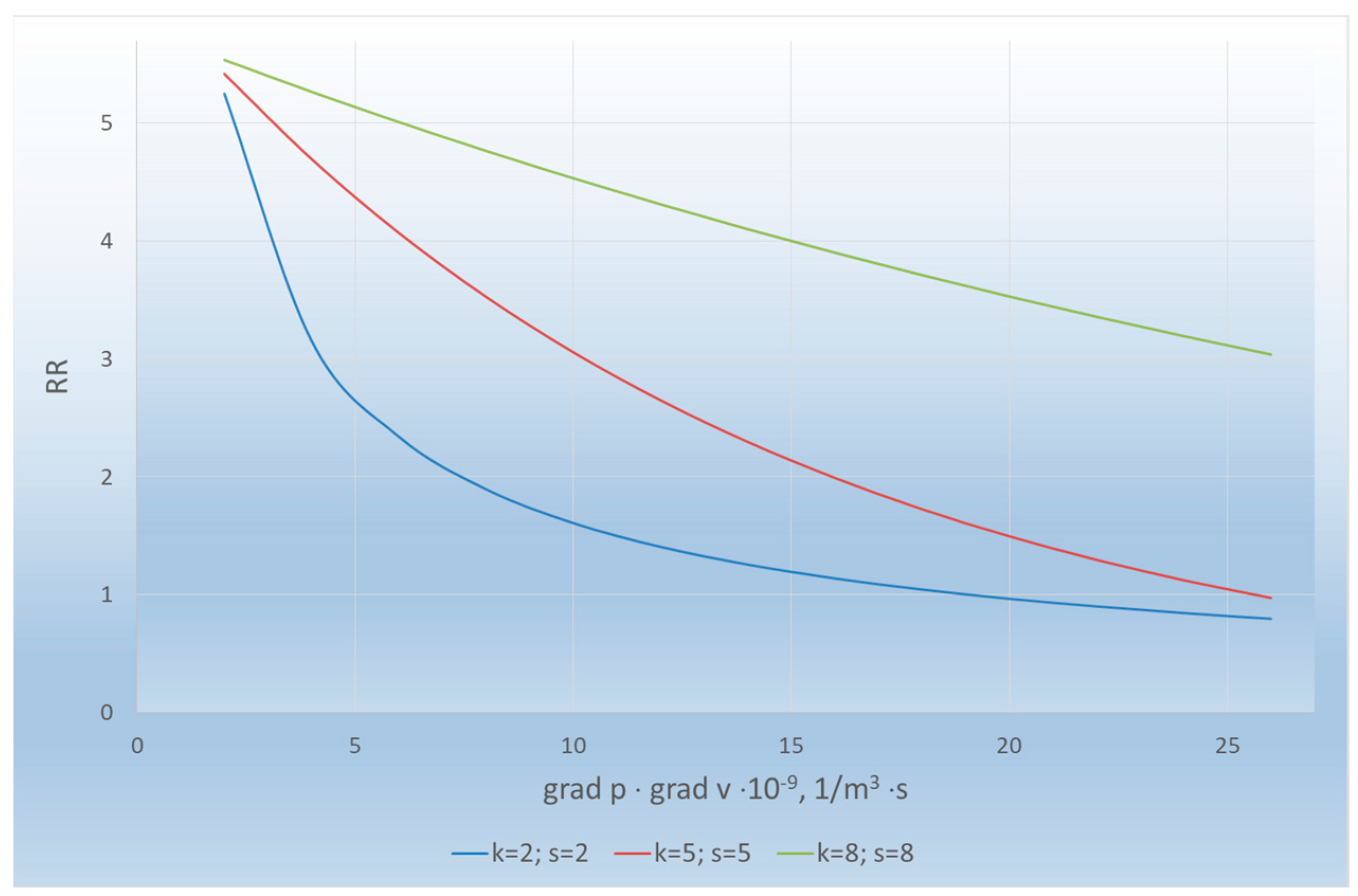
| Pedestrian crossings and traffic lights quantities in the controlled stretch, unit | k/s | 2/2 | 5/5 | 8/8 |
| Parameter for Modeling | Grad p · Grad v · 10−9, 1/m3·s | |||||||||||
|---|---|---|---|---|---|---|---|---|---|---|---|---|
| 2.5 | 5 | 7.5 | 10 | 12.5 | 15 | 17.5 | 20 | 22.5 | 25 | 27.5 | ||
| Vehicle length, m | 4 | 10 | 9.3 | 8.6 | 8 | 7.3 | 6.6 | 6 | 5.3 | 4.6 | 3.3 | 2.6 |
| 12 | 24 | 22.3 | 20.6 | 19 | 17.3 | 15.6 | 14 | 12.3 | 10.6 | 7.3 | 5.6 | |
| 20 | 50 | 49 | 48 | 47 | 46 | 45 | 44 | 43 | 42 | 40 | 39 | |
| Vehicle weight, kg | 2000 | 3.84 | 3.2 | 2.64 | 2.15 | 1.74 | 1.4 | 1.12 | 0.91 | 0.78 | 0.72 | 0.7 |
| 10,000 | 6 | 4.15 | 3.17 | 2.7 | 2.36 | 2.12 | 1.94 | 1.8 | 1.68 | 1.58 | 1.5 | |
| 18,000 | 19.7 | 14.07 | 11.55 | 10 | 9 | 8.25 | 7.65 | 7.17 | 6.77 | 6.43 | 6.1 | |
| Vehicle engine power, kW | 100 | 5.13 | 4.65 | 4.18 | 3.73 | 3.29 | 2.88 | 2.48 | 2.1 | 1.73 | 1.38 | 1.05 |
| 150 | 5.65 | 5.13 | 4.63 | 4.15 | 3.7 | 3.24 | 2.8 | 2.38 | 1.98 | 1.6 | 1.22 | |
| 200 | 6.35 | 5.8 | 5.25 | 4.72 | 4.21 | 3.72 | 3.25 | 2.8 | 2.35 | 1.92 | 1.51 | |
| Driver’s reaction time to the traffic situation, s | 0.6 | 5 | 4 | 3.17 | 2.52 | 2 | 1.6 | 1.27 | 1 | 0.8 | 0.64 | 0.51 |
| 1.0 | 7.18 | 5.7 | 4.52 | 3.6 | 2.85 | 2.26 | 1.8 | 1.42 | 1.13 | 0.9 | 0.71 | |
| 1.4 | 11.44 | 9.1 | 7.24 | 5.75 | 4.58 | 3.64 | 2.9 | 2.3 | 1.83 | 1.45 | 1.15 | |
| Vehicle maneuver time according to traffic situation changes, s | 4 | 0.84 | 0.71 | 0.6 | 0.5 | 0.4 | 0.34 | 0.28 | 0.25 | 0.22 | 0.21 | 0.2 |
| 7 | 1.61 | 1.4 | 1.21 | 1.04 | 0.9 | 0.8 | 0.7 | 0.62 | 0.58 | 0.55 | 0.5 | |
| 10 | 5.7 | 5.0 | 4.37 | 3.8 | 3.25 | 2.76 | 2.32 | 1.93 | 1.58 | 1.29 | 1.0 | |
| Total delays time driving route, s | 50 | 8.75 | 8.23 | 7.7 | 7.18 | 6.6 | 6.14 | 5.62 | 5.1 | 4.58 | 4.06 | 3.54 |
| 150 | 12.5 | 11.7 | 10.91 | 10.12 | 9.3 | 8.54 | 7.75 | 6.95 | 6.16 | 5.37 | 4.58 | |
| 250 | 22.5 | 21.0 | 19.54 | 18.06 | 16.58 | 15.1 | 13.62 | 12.14 | 10.66 | 9.18 | 7.7 | |
| Lanes quantity on the roadway, unit | 1 | 9.6 | 8.69 | 7.86 | 7.11 | 6.44 | 5.82 | 5.27 | 4.77 | 4.31 | 3.9 | 3.53 |
| 2 | 14.04 | 12.54 | 11.2 | 10.0 | 8.93 | 7.98 | 7.12 | 6.36 | 5.68 | 5.07 | 4.53 | |
| 3 | 23.07 | 20.42 | 18.07 | 16.0 | 14.16 | 12.53 | 11.09 | 9.82 | 8.69 | 7.69 | 6.81 | |
| Pedestrian crossings and traffic lights quantities in the controlled stretch, unit | 2/2 | 5.25 | 3.15 | 2.34 | 1.9 | 1.6 | 1.4 | 1.25 | 1.13 | 1.04 | 0.96 | 0.9 |
| 5/5 | 5.41 | 4.7 | 4.0 | 3.52 | 3.05 | 2.65 | 2.3 | 2 | 1.72 | 1.49 | 1.29 | |
| 8/8 | 5.53 | 5.26 | 5.0 | 4.76 | 4.53 | 4.31 | 4.1 | 3.9 | 3.71 | 3.53 | 3.35 | |
Disclaimer/Publisher’s Note: The statements, opinions and data contained in all publications are solely those of the individual author(s) and contributor(s) and not of MDPI and/or the editor(s). MDPI and/or the editor(s) disclaim responsibility for any injury to people or property resulting from any ideas, methods, instructions or products referred to in the content. |
© 2023 by the authors. Licensee MDPI, Basel, Switzerland. This article is an open access article distributed under the terms and conditions of the Creative Commons Attribution (CC BY) license (https://creativecommons.org/licenses/by/4.0/).
Share and Cite
Vojtov, V.; Muzylyov, D.; Karnaukh, M.; Kravtcov, A.; Goryayinov, O.; Gorodetska, T.; Ivanov, V.; Pavlenko, I. Modeling of Traffic Flows Sustainability on Highway Network Stretches. Appl. Sci. 2023, 13, 9307. https://doi.org/10.3390/app13169307
Vojtov V, Muzylyov D, Karnaukh M, Kravtcov A, Goryayinov O, Gorodetska T, Ivanov V, Pavlenko I. Modeling of Traffic Flows Sustainability on Highway Network Stretches. Applied Sciences. 2023; 13(16):9307. https://doi.org/10.3390/app13169307
Chicago/Turabian StyleVojtov, Viktor, Dmitriy Muzylyov, Mykola Karnaukh, Andriy Kravtcov, Oleksiy Goryayinov, Tetiana Gorodetska, Vitalii Ivanov, and Ivan Pavlenko. 2023. "Modeling of Traffic Flows Sustainability on Highway Network Stretches" Applied Sciences 13, no. 16: 9307. https://doi.org/10.3390/app13169307
APA StyleVojtov, V., Muzylyov, D., Karnaukh, M., Kravtcov, A., Goryayinov, O., Gorodetska, T., Ivanov, V., & Pavlenko, I. (2023). Modeling of Traffic Flows Sustainability on Highway Network Stretches. Applied Sciences, 13(16), 9307. https://doi.org/10.3390/app13169307