Article

Object Detection for Brain Cancer Detection and Localization

1
Department of Medicine and Health Sciences “Vincenzo Tiberio”, University of Molise, 86100 Campobasso, Italy
2
Institute for Informatics and Telematics, National Research Council of Italy, 56124 Pisa, Italy
3
Department of Engineering, University of Sannio, 82100 Benevento, Italy
*
Author to whom correspondence should be addressed.
Appl. Sci. 2023, 13(16), 9158; https://doi.org/10.3390/app13169158
Submission received: 17 July 2023 / Revised: 4 August 2023 / Accepted: 10 August 2023 / Published: 11 August 2023

Abstract

:
Brain cancer is acknowledged as one of the most aggressive tumors, with a significant impact on patient survival rates. Unfortunately, approximately 70% of patients diagnosed with this malignant cancer do not survive. This paper introduces a method designed to detect and localize brain cancer by proposing an automated approach for the detection and localization of brain cancer. The method utilizes magnetic resonance imaging analysis. By leveraging the information provided by brain medical images, the proposed method aims to enhance the detection and precise localization of brain cancer to improve the prognosis and treatment outcomes for patients. We exploit the YOLO model to automatically detect and localize brain cancer: in the analysis of 300 brain images we obtain a precision of 0.943 and a recall of 0.923 in brain cancer detection while, relating to brain cancer localization, an mAP_0.5 equal to 0.941 is reached, thus showing the effectiveness of the proposed model for brain cancer detection and localization.

1. Introduction

Brain cancer encompasses the growth of abnormal cells or a cluster of cells within the brain or its adjacent structures. Brain tumors, which fall under the category of brain cancer, can be classified as either malignant (i.e., cancerous) or benign (i.e., healthy). Malignant brain tumors have the ability to invade neighboring tissues and potentially metastasize to other parts of the body, while benign tumors typically do not invade surrounding tissues or metastasize.
It is indeed true that brain tumors pose a significant risk for cancer-related fatalities in children under the age of 20. As a matter of fact, brain tumors have surpassed acute lymphoblastic leukemia as the leading cause of solid tumor cancer deaths within this age group. This highlights the critical importance of understanding and addressing brain tumors in the field of pediatric oncology. Comprehensive knowledge and advancements in diagnosing and treating brain tumors are crucial to improve outcomes and enhance the quality of life of affected children (http://blog.braintumor.org/, accessed on 8 August 2023).
Brain tumors do indeed represent a substantial cause of solid-tumor cancer-related deaths among young adults aged 20 to 39. They rank as the third leading cause of solid tumor cancer fatalities in this age bracket [1]. Each year, over 5000 individuals succumb to brain tumors, highlighting the significant toll this disease takes on affected individuals.
Moreover, in the United Kingdom, there is an estimated population of at least 102,000 children and adults currently living with brain tumors. This statistic emphasizes the prevalence of brain tumors and the profound impact they have on individuals and their families. The number of people living with brain tumors underscores the need for continued research [2], improved treatments [3], and support for affected individuals to enhance their quality of life and overall outcomes (https://www.cancerresearchuk.org/health-professional/cancer-statistics/statistics-by-cancer-type/brain-other-cns-and-intracranial-tumours, accessed on 8 August 2023).
Brain tumors can indeed have a profound impact on life expectancy. On average, individuals diagnosed with brain tumors may experience a reduction in life expectancy of approximately 20 years. This reduction in life expectancy is considered one of the highest among all types of cancer.
However, it is crucial to note that survival rates for brain tumors can vary significantly depending on various factors. These factors include the specific type of tumor, its grade (degree of malignancy), location, and individual characteristics of the patient. The mentioned statistic stating that only 19% of adults survive for five years after a cancer diagnosis is a general estimate and may not apply uniformly to all types and stages of brain tumors. Survival rates can vary widely, and it is important to consider individual circumstances and factors when assessing a prognosis and discussing treatment options with healthcare professionals (https://www.cancer.net/cancer-types/brain-tumor/statistics, accessed on 8 August 2023).
Brain cancers can certainly have a significant impact on both physical and cognitive abilities due to their location within the control center of the brain, which governs movement and emotion. The brain plays a vital role in coordinating various bodily functions, including motor skills, sensory perception, cognition, and emotional regulation. When brain tumors develop in these crucial areas, they can disrupt the normal functioning of these processes [4].
Treatment approaches for brain tumors, such as surgery, radiation therapy, and chemotherapy, aim to target and manage the tumors while minimizing damage to surrounding healthy brain tissue [5,6]. In addition to these treatments, rehabilitation therapies, such as physical therapy, occupational therapy, and speech therapy, may be employed to help patients regain or adapt to changes in their physical and cognitive abilities. These rehabilitation therapies can assist in restoring or maximizing functional abilities, promoting independence, and improving the overall quality of life for individuals affected by brain tumors.
In recent years, we witnessed a growing interest in artificial intelligence, with particular regard to object detection, a computer vision technique that involves identifying and locating objects of interest within digital images or video frames. It represents a fundamental task in many applications, including autonomous vehicles, surveillance systems, image and video analysis [7], robotics, and more [8].
The aim of object detection is to not only recognize the presence of objects but also determine their precise locations and boundaries within an image or a video. This is typically achieved by drawing bounding boxes around the objects and labeling them with corresponding class labels, indicating the type of objects detected (e.g., cars, pedestrians, animals).
Starting from these considerations, in this paper, we investigate the possibility to detect and localize brain cancer starting from magnetic resonance images (MRI), analyzed with object detection techniques. In particular, the You Only Look Once (YOLO) object detection model is exploited for this purpose. The key idea behind the YOLO model is that it treats object detection as a regression problem, where a neural network is trained to directly predict the bounding boxes and class probabilities of objects within an image. Unlike traditional object detection methods that use complex multi-stage pipelines, YOLO uses a single neural network to simultaneously predict the bounding boxes and class probabilities for multiple objects in an image. We exploit this model by considering its efficiency and real-time performance and its ability to achieve high accuracy while maintaining fast inference speeds.
The paper proceeds as follows: in the next section the proposed method for brain cancer detection and localization is presented; in Section 3, the experimental analysis results are discussed; in Section 4, the state-of-the-art literature is presented; and finally, in the last section, the conclusion and future research lines are drawn.

2. The Method

In this section, we describe the proposed method for automatic detection and localization of brain cancer by analyzing brain MRIs. The focus of this paper is specifically on brain MRIs, but the proposed method can be readily applied to other types of bioimages, such as those related to the lung or other organs.
Figure 1 shows the workflow of the proposed method, designed to detect and localize brain cancer.
In order to build an effective deep learning model for the detection and localization of brain cancer from MRI scans, it is essential to have a dataset that consists of brain cancer MRIs along with corresponding annotations (i.e., bounding boxes) indicating the localization of the cancerous regions.
We highlight the importance of having a high-quality dataset that includes both the MRIs and precise annotations of the cancer localization. Such a dataset serves as the foundation for training the object detection model effectively. By having accurate annotations, the model can learn to identify and locate the specific regions within the brain MRI scans that indicate the presence of cancer.
Having a reliable and well-annotated dataset is crucial in the development of a robust and accurate object detection model for brain cancer detection and localization. It ensures that the model is trained on representative and informative data, enabling it to make precise predictions when applied to new, unseen MRI scans.
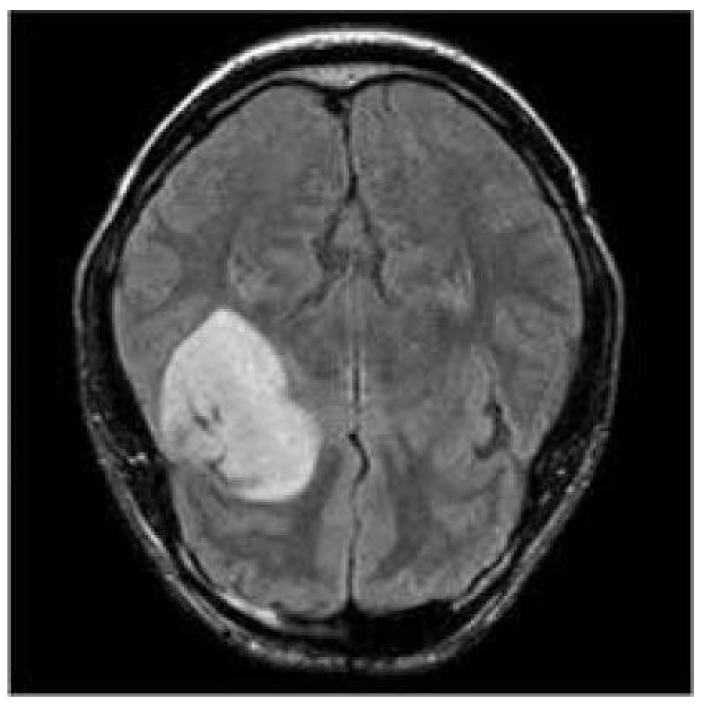
In Figure 2, we show an example of an MRI related to brain cancer.
Within the MRI shown in Figure 2, it is possible to observe a lighter gray, almost white area on the left side of the image, indicating where the brain tumor is located.
In order to construct a model that is both efficient and capable of accurately predicting unseen images, a diverse dataset was compiled. This dataset comprises images captured from various angles, under different conditions, and featuring different types of tumors. Each image within the dataset has a unique size. However, to facilitate further analysis, a preprocessing step is required to resize all the images to a consistent dimension.
Once the images are obtained, we need to define the class for the detection of the bounding box for the brain MRI: in this case, we have one class that is tumor, related to the brain cancer presence.
We annotated each image by drawing bounding boxes around each detected object. This annotation process was carried out using the Labelbox web application (https://labelbox.com/, accessed on 8 August 2023), i.e., a platform designed to perform data annotation tasks.
The subsequent step involves image augmentation, which refers to a collection of techniques that expand the existing dataset without the need for gathering new samples. Data augmentation involves applying controlled random modifications to existing images and generating modified versions of them. This technique is commonly employed in training artificial neural networks, as it enables them to “learn” more effectively and accurately as the size of the training dataset grows.
Specifically, we employ data augmentation techniques to generate modified images of brain MRIs with controlled random variations, such as rotations, flips, cuts, and trims. The objective behind applying data augmentation in this context is to make the model capable of effectively detecting tumors regardless of their position within the image. Additionally, augmented data are utilized to address the issue of overfitting, which occurs when a statistical model becomes too specialized in fitting the observed data sample due to an excessive number of parameters compared to the number of observations.
By introducing variations through data augmentation, the structured neural network can learn to recognize recurring patterns from the augmented data, rather than simply memorizing specific examples. This helps the model develop more generalized rules and reduces the chances of misclassifying unseen patterns. Data augmentation plays a crucial role in improving the model’s ability to generalize and perform well on unseen images.
After acquiring the augmented brain MRIs, along with the corresponding information regarding cancer localization (i.e., the class) and bounding boxes, the next step is to develop a deep learning model.
As stated in the introduction section, in this paper we utilize the YOLO model [9,10,11].
The YOLO model [12], which was introduced by J. Redmon et al. in 2016, serves as the pioneering one-stage deep learning detector. YOLO is specifically designed as an object detection model that performs both image classification and accurate object localization within the images.
The distinctive feature of YOLO, setting it apart from other networks, is its self-contained pipeline that carries out the entire process independently. In YOLO, the input is an image, and the output consists of two components: a bounding box vector and the associated class prediction for each cell.
During analysis, each image is divided into an S × S grid of cells. If an object falls within the center of a cell, that cell is responsible for detecting the object. The bounding box prediction consists of five components: (x, y, w, h, confidence). The (x, y) coordinates represent the center of the bounding box relative to the cell’s position in the grid. These coordinates are normalized to values between 0 and 1. The dimensions of the box (w, h) are also normalized to a range of [0, 1], relative to the image dimensions. In total, the predictions of the bounding boxes result in S × S × B × 5 outputs, where B denotes the number of bounding boxes predicted per cell [13].
When compared to existing object detection models, YOLO has been demonstrated to be notably faster [14,15].
This efficiency is primarily achieved because YOLO performs the recognition task in a single phase, without dividing it into multiple stages. Instead of having separate stages for region proposal and object classification, YOLO directly predicts bounding boxes, object probabilities, and classes of objects present in the input image. This streamlined approach contributes to the significant speed advantage of YOLO compared to other object detection models.
We choose to utilize the YOLO model for several reasons when compared to other deep learning models for object detection. Despite the fact that YOLO may have more localization errors [16], it exhibits a lower tendency to identify false positives in the background of an image. Furthermore, YOLO is significantly faster than many other models [13,17]. These factors contribute to YOLO being widely regarded as one of the top convolutional neural network models for object detection.
It is important to note that there exist multiple versions of the YOLO model. For this paper, we consider and implement YOLOv8s (https://docs.ultralytics.com/, accessed on 8 August 2023) using the PyTorch framework (https://pytorch.org/, accessed on 8 August 2023).
The reason why we chose the YOLOv8 model is the significant improvement over previous YOLO models in a number of ways, including the following:
  • Anchor-free detection. YOLOv8 does away with the use of anchor boxes, which were a key component of previous YOLO models. Anchor boxes are pre-defined bounding boxes that are used to classify objects in an image. However, anchor boxes can be restrictive, and they can make it difficult for the model to learn to detect objects that are not well-represented by the anchor boxes. YOLOv8 uses a new technique called anchor-free detection, which allows the model to learn to detect objects of any size and shape.
  • C3 convolutions. YOLOv8 uses a new type of convolution called C3 convolutions. C3 convolutions are more efficient than traditional convolutions, and they allow the model to learn more complex features.
  • Mosaic augmentation. YOLOv8 uses a new type of data augmentation called mosaic augmentation. Mosaic augmentation creates a new image by stitching together four randomly cropped images. This helps the model to learn to generalize to different object appearances and different lighting conditions.
As a result of these improvements, YOLOv8 is able to achieve state-of-the-art object detection performance on a number of benchmarks. For example, YOLOv8 achieves a mean average precision (mAP) of 50.1% on the COCO dataset, which is a benchmark for object detection.
Adopting YOLO in medical image classification offers several benefits and advantages:
  • Real-time detection: YOLO is known for its real-time object detection capabilities. In the context of medical image classification, this means that YOLO can quickly and efficiently identify abnormalities, lesions, or specific medical conditions in real-time, allowing for faster diagnosis and treatment planning.
  • Object localization: YOLO is designed to not only classify objects but also precisely localize them within the image. In medical imaging, this localization can be crucial for identifying the exact location and extent of abnormalities, aiding medical professionals in making accurate diagnoses.
  • Handling multiple classes: YOLO can handle multiple classes or categories simultaneously. In medical image classification, this is advantageous as it allows the model to detect and classify various medical conditions or abnormalities within a single image.
  • Single-pass approach: YOLO follows a single-pass approach, making predictions in one pass through the neural network. This design makes YOLO faster and more computationally efficient compared to some other object detection models, making it suitable for large-scale medical image datasets.
  • Transfer learning: YOLO can leverage pre-trained models on large image datasets (e.g., ImageNet) for feature extraction and then fine-tune the model on medical image datasets. This transfer learning approach allows the model to learn relevant features from general images and then adapt them to medical images, even with limited labeled medical data.
  • Generalizability: YOLO has shown promising generalization capabilities across different domains and tasks. This is essential in medical image classification, as medical datasets can vary in terms of image quality, patient demographics, and equipment, and a model that can generalize well is desirable.
  • Ongoing research and development: YOLO is an actively researched object detection architecture, and advancements in its design and training methodologies continue to improve its performance. This ongoing research ensures that adopting YOLO in medical image classification can benefit from the latest advancements in computer vision and deep learning.
Overall, the use of YOLO in medical image classification can lead to faster, more accurate, and more efficient diagnosis and analysis of medical conditions, ultimately improving patient care and outcomes.
The architecture of the YOLOv8s is shown in Table 1.
As depicted in Figure 1, the YOLO network architecture comprises two main components: the backbone and the head. The backbone, as illustrated in Table 1, is a convolutional neural network responsible for extracting and consolidating image features at various scales or granularities. On the other hand, the head, also shown in Table 1, takes in features from the backbone and carries out the box and class prediction processes.
Situated between the backbone and the head is the neck, which consists of a series of layers that blend and merge image features before forwarding them to the prediction stage. This intermediate step allows for effective combination and transformation of features, enhancing the network’s ability to make accurate predictions.
Overall, the YOLO architecture integrates these components to enable comprehensive feature extraction, feature fusion, and prediction steps, contributing to its object detection capabilities.
Once the YOLO model is trained, it will be able to perform the following operations on unseen brain MRIs:
  • Classify the image as cancerous;
  • Detect the area (i.e., localize) related to brain cancer;
  • Assign a probability of the cancer presence.

3. Experimental Analysis

In this section, we present the results of the proposed experimental analysis, which aims to demonstrate the effectiveness of the proposed YOLO model in detecting and localizing brain cancer.

3.1. The Dataset

We obtained the real-world data that we analyzed from a repository freely available for research purposes [18]. The exploited dataset is composed of 300 brain MRIs. We considered 70% of the dataset for training (210 images), 20% for validation (60 images), and the remaining 10% for testing (30 images). The dataset is labeled with the “tumor” label, with the detail related to the bounding box related to the label localization.
The dataset is composed of brain images relating to different types of brain tumors (i.e., Meningioma, Pituitary, and Glioma), of different dimensions and located in different areas of the brain. Considering that different types of tumors were considered (and that in the dataset they are represented with the same number of images), the images of healthy subjects are equal to 25% of the total images.
We resized all the images to the dimension of 512 × 512 pixels. Regarding the model parameters, we used a batch size of 16 and we set the number of epochs to 50. As optimizer, the stochastic gradient descent (SGD) was exploited. We set the patience parameter to 50, the workers to 8, the maximum number of detections per image to 300, the momentum to 0.937, and the intersection over union (IoU) threshold for Non Maxima Suppression (NMS) to 0.7.
We utilized the Roboflow web application to perform data augmentation (https://roboflow.com/, accessed on 8 August 2023) by randomly rotating the pictures 90° clockwise, 90° counterclockwise, and upside down.
Roboflow is a platform that facilitates developers in managing computer vision projects by providing data management capabilities. It enables the integration of images along with annotations created on Labelbox and offers the ability to apply various transformations to the images.

3.2. The Results

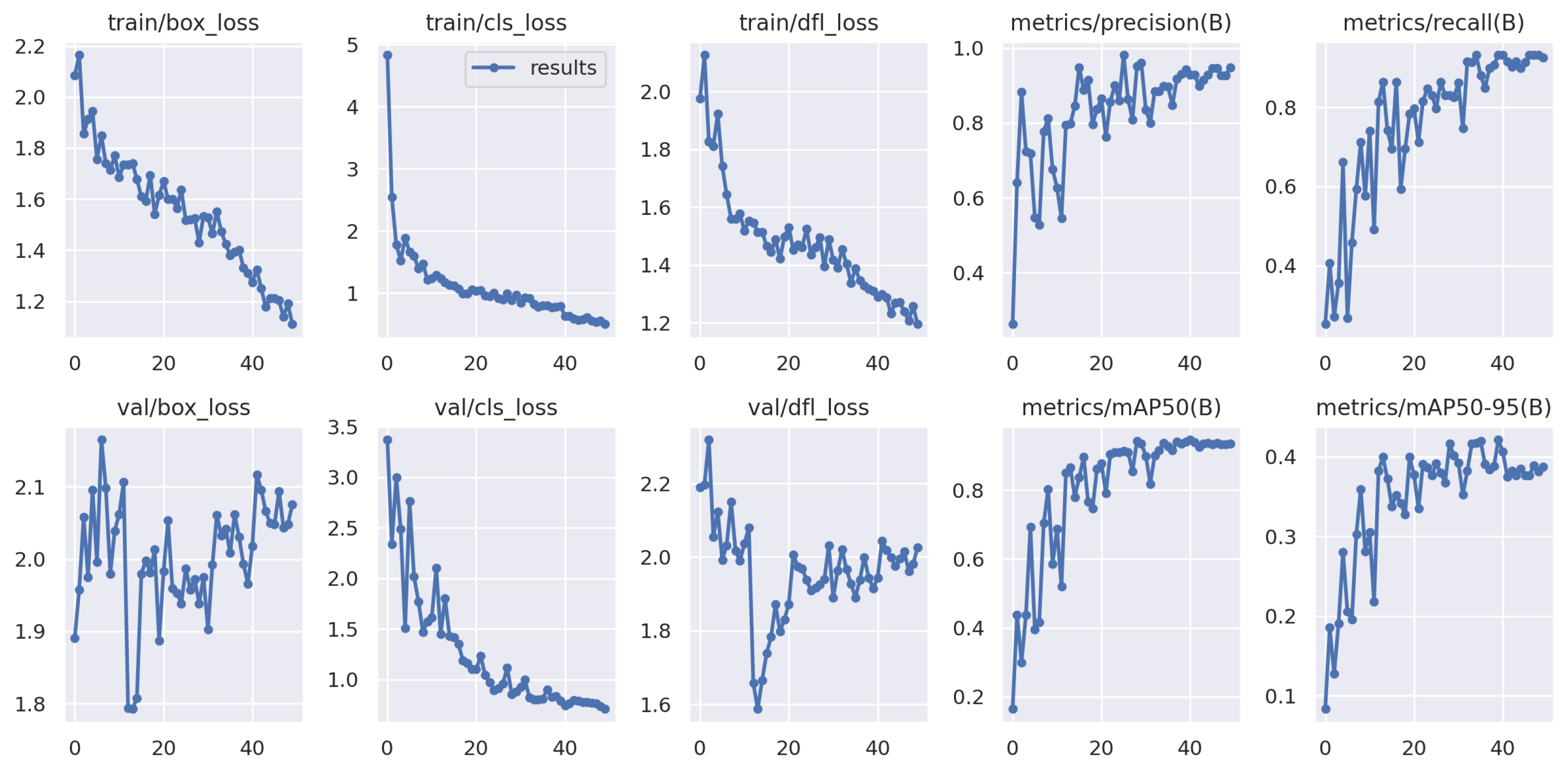
Figure 3 presents a collection of plots illustrating the performance of the proposed model for detecting and localizing brain cancer.
The 50 epochs were completed in 0.095 h by exploiting an NVIDIA Tesla T4 graphic card with 16 GB of memory, with a CUDA Version equal to 12.0. Moreover, we used the 3.10.12 version of the Python compiler with the Torch library (version 2.0.1).
In detail, in Figure 3 there are 12 plots, 6 plots in each line.
The first plot in Figure 3 (i.e., the Box plot) shows the box loss metric trend. The plot represents the training step, where the values of the loss are plotted on the y-axis (ordinates), and the different epochs are represented on the x-axis (abscissa). In object detection tasks, which involve both localization and classification, the primary method for localizing multiple objects in an image is through bounding boxes. The loss function used in this context calculates the error between the predicted bounding boxes and the ground truth bounding boxes. The goal of this loss function is to minimize the discrepancy between the predicted and actual bounding boxes. As the loss decreases over epochs, it indicates that the network is learning and improving its ability to accurately predict tight bounding boxes.
The second plot in Figure 3 (i.e., Objectness) shows the objectness loss. In the training step, the plot represents the behavior of the objectness and class score in the deep learning model for object detection. The objectness refers to the confidence of the model in the presence of an object within a given bounding box. On the other hand, the class score represents the conditional probability of a specific class, given that an object exists in that box. The total confidence score for each class is obtained by multiplying the objectness and the class score. In this scenario, it is desirable for the objectness to decrease towards zero as the number of epochs increases. This indicates that the model becomes more confident in accurately detecting the presence of objects. Therefore, the plot shows the trend of the objectness scores over the epochs during the training process.
The third plot in Figure 3 is related to the Classification. In the training step, the plot illustrates the classification aspect of the object detection task. The objective of classification is twofold: to determine whether an object is present in the image and to identify the specific class of the object. In the plot, the loss for classification is depicted, which assesses the accuracy of the classification for each predicted bounding box. Each bounding box can potentially contain an object class or be classified as “background”. The loss function commonly employed for classification tasks is the cross-entropy loss. The plot showcases the progression of the cross-entropy loss over the epochs during the training phase. It reflects how well the model is learning to correctly classify objects within the predicted bounding boxes.
The val Box, the val Objectness, and the val Classification plots are related to the loss trends for the box loss metric, for the objectness, and for the classification loss relating to the testing dataset: as in the previous plots, in these cases we expect a decreasing trend when the number of epochs increases.
The fourth and the fifth plots (i.e., Precision and Recall) show the value for each epoch for the precision and the recall metrics.
Precision is a metric that quantifies the proportion of positive predictions that are accurately classified. It takes into consideration the occurrence of false positives, which refers to cases that were incorrectly identified as positive or flagged for inclusion. Precision can be computed as
P r e c i s i o n = T P T P + F P
Recall, also known as sensitivity or true positive rate, is a metric that assesses the proportion of actual positive instances that were correctly predicted as positive by the model. It takes into account false negatives, which are cases that should have been flagged for inclusion as positive but were incorrectly classified as negative by the model. Recall can be computed as
R e c a l l = T P T P + F N
As the number of epochs increases, both precision and recall should exhibit an upward trend. This trend, indeed, is demonstrated in the graphs depicting these metrics. Notably, precision and recall values ranging from 0 to 1 are considered desirable. Achieving precision and recall values exceeding 0.9 in the final epochs is particularly noteworthy, as it indicates that the deep learning model has effectively learned and achieved high performance in the task at hand.
Specificity (also called true negative rate) represents the probability that an actual negative will test negative. It is computed as follows:
S p e c i f i c i t y = T N T N + F P
AP (i.e., average precision) is a widely used metric for evaluating the accuracy of object detectors: it computes the average precision value by considering the recall values ranging from 0 to 1. Average precision provides a comprehensive measure of the model’s performance across different recall levels and is a valuable metric for assessing the accuracy and effectiveness of object detection algorithms.
The computation of mean average precision (mAP) involves several components, including intersection over union (IOU), precision, recall, precision–recall curve, and average precision (AP).
In object detection, models predict both the bounding box and the category of objects within an image. IOU is utilized to evaluate whether the predicted bounding box accurately matches the ground truth bounding box. It quantifies the overlap between the predicted and actual bounding boxes.
The precision–recall curve showcases the trade-off between precision and recall for various classification thresholds. It provides insights into the model’s performance across different operating points.
AP (average precision) is the average precision calculated at each point on the precision–recall curve. It summarizes the model’s overall performance in object detection.
To calculate mAP, the AP values obtained from multiple classes or categories are averaged, providing a comprehensive evaluation of the model’s performance across all object classes.
IOU (intersection over union) is a measure that quantifies the extent of overlap between two bounding boxes. It is calculated as the ratio of the intersection area to the union area of the two bounding boxes. The IOU value ranges from 0.0 to 1.0, where 1.0 indicates a perfect match or complete overlap, and 0.0 indicates no overlap at all.
The formula for computing the IOU is defined as follows:
I O U = A r e a o f I n t e r s e c t i o n A r e a o f U n i o n
This formula compares the regions covered by two bounding boxes and provides a standardized measure of their overlap, which is useful in evaluating the accuracy of bounding box predictions in object detection tasks.
During the evaluation of object detection models, it is essential to establish a criterion for determining successful recognition based on the overlap of bounding boxes with ground truth data. IOUs (intersection over union) are employed for this purpose.
The metric [email protected] represents the accuracy when an IOU threshold of 0.5 is used. In other words, if the overlap between the predicted bounding box and the ground truth bounding box exceeds 50%, the detection is considered successful.
As the IOU threshold increases, the required accuracy for bounding box detection becomes stricter, making it more challenging to achieve. Consequently, a higher IOU threshold, such as [email protected], typically yields a lower mAP value compared to [email protected]. This indicates that achieving accurate bounding box detection with a higher overlap requirement is more difficult.
The mean average precision (mAP) is calculated as an average of the average precision (AP) values. Each AP value represents the precision–recall trade-off for a specific class in object detection.
To compute mAP, the AP values obtained for all classes are further averaged, resulting in a single metric that summarizes the overall performance of the object detection model across multiple object classes. This aggregation allows for a comprehensive evaluation of the model’s accuracy and effectiveness in detecting objects across various categories.
Figure 3 shows, in the [email protected] and the [email protected]:0.95 plots, respectively, the mAP value for IOU = 50 and IOU ranging from 50 to 95 (i.e., this value represents different IoU thresholds from 0.5 to 0.95, with a step size equal to 0.05 on average mAP).
Table 2 shows the values obtained for Precision, Recall, mAP_0.5, and mAP_0.5:0.95 metrics.
From Table 2, we can note that the precision and the recall metrics obtain interesting values in both the training and testing steps: as a matter of fact, the precision is equal to 0.948 in training and 0.943 in testing, while the recall is equal to 0.926 in training and 0.932 in testing. Furthermore, the mAP_0.5 obtains good performances, equal to 0.935 and 0.941, respectively, in the training and in the testing step.
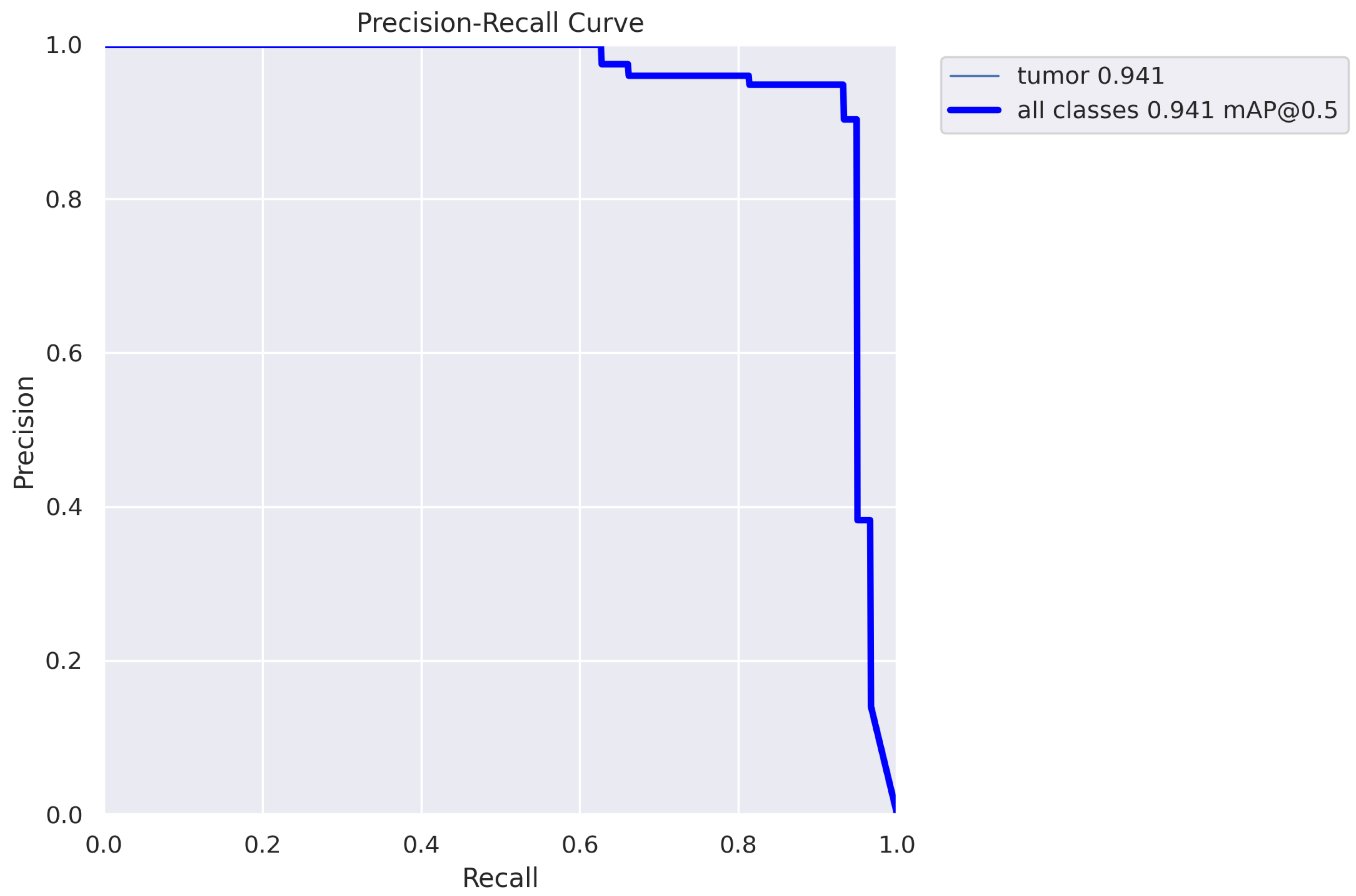
To thoroughly analyze the performance achieved in terms of precision and recall, let us delve into the details of the results; Figure 4 displays the precision and recall values plotted on the precision–recall graph.
By examining the precision and recall values obtained, we can assess the model’s performance in terms of both accuracy and completeness. A high-precision value indicates a low false positive rate, while a high recall value indicates a low false negative rate. Striking a balance between precision and recall is crucial for achieving an effective object detection model.
The trend of the precision–recall plot is generally expected to be monotonically decreasing. This is because there is typically a trade-off between precision and recall in object detection tasks. Increasing one metric often leads to a decrease in the other. The trade-off between precision and recall arises from the nature of the detection problem. Setting a higher threshold for classification as a positive prediction may increase precision but decrease recall, as only highly confident predictions are accepted. Conversely, lowering the threshold to include more predictions can increase recall but potentially decrease precision by including more false positives. However, it is important to note that there can be exceptions and variations in the precision–recall graph. In certain cases, due to specific circumstances or insufficient data, the graph may not exhibit a strictly monotonically decreasing trend. These exceptions can arise from factors such as class imbalance, outliers, or unique characteristics of the dataset. Therefore, while the monotonically decreasing trend is typical, it is essential to carefully analyze the specific characteristics of the precision–recall graph in each scenario. From the plot in Figure 4, we can see that this plot exhibits a decreasing trend. The precision–recall plot also shows the area under the curve (AUC) values related to the brain tumor detection [email protected]. As previously stated, the precision–recall trend is expected to be monotonically decreasing: this behavior is shown by the precision–recall plot related to a value of [email protected] (with an AUC equal to 0.941).
Figure 5 presents the normalized confusion matrix of the proposed YOLO model. The confusion matrix is utilized to gain a more detailed understanding of the model’s performance across different classes, identifying both the best-performing and worst-performing classes. Furthermore, the confusion matrix helps in identifying the specific instances that have been misclassified and provides insights into the misclassification patterns. By examining the confusion matrix, one can observe the distribution of predictions and actual labels for each class. It allows for a comprehensive evaluation of the model’s accuracy, highlighting areas where misclassifications are more prominent and identifying potential sources of errors. This information is valuable in guiding improvements and refining the model’s performance in object detection tasks.
From the normalized confusion matrix, we can confirm the effectiveness of the model for brain cancer detection and localization; as a matter of fact, the model is able to detect the brain tumor area and to discern between the brain and image background. In the case of the YOLO confusion matrix, the columns represent the predicted classes, and they are normalized (in our case the classes are tumor and background, i.e., everything that is not part of the images relating to the tumor is therefore healthy tissue). As a result, the sum of each of the columns would be equal to 1. Regarding the background class, according to the YOLO developers, it is not predicted by the model.

3.3. Prediction Examples

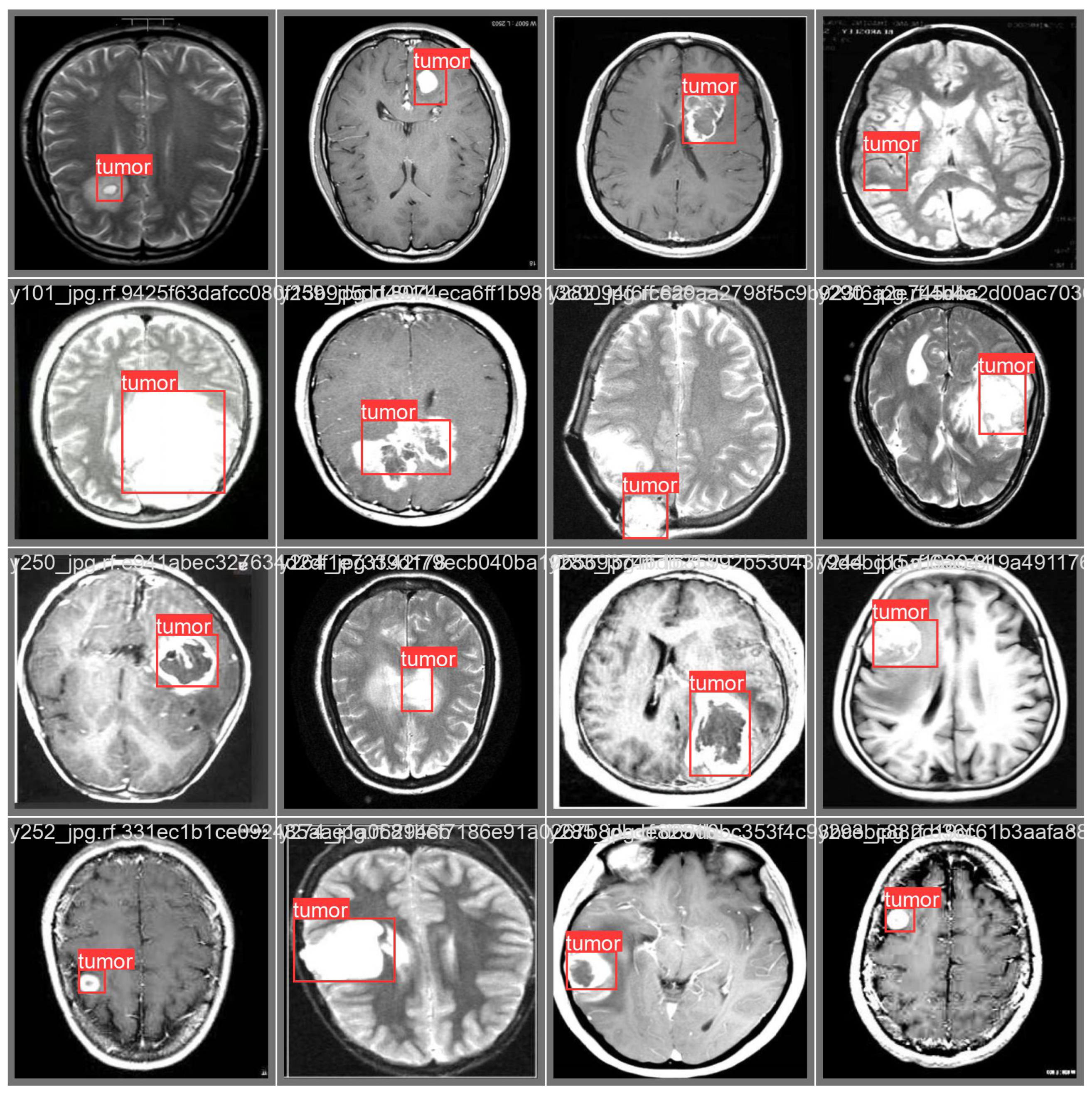
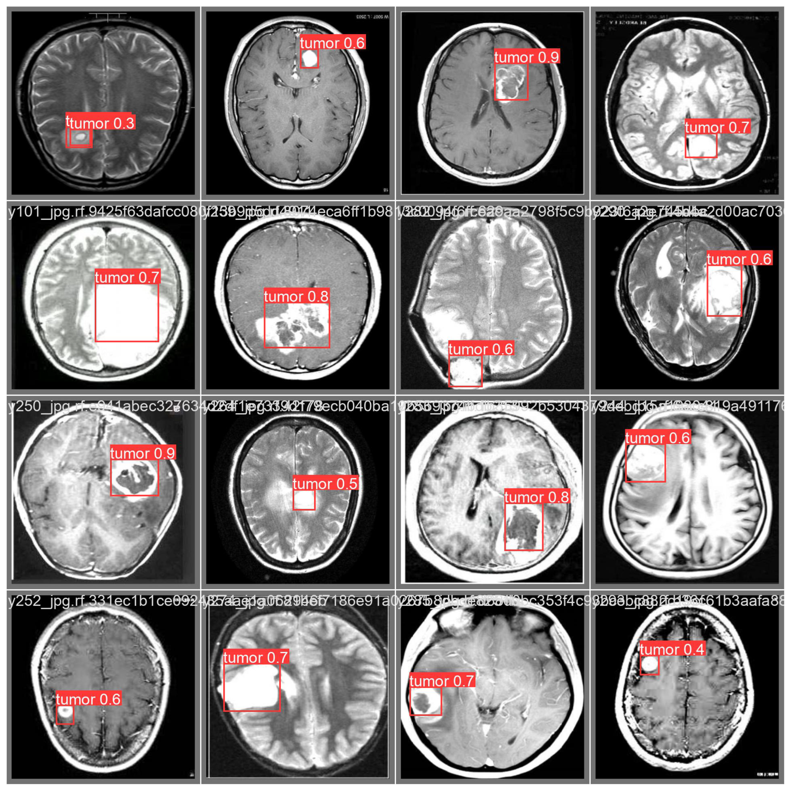
With the aim to show how the proposed method can be employed in the real world, in Figure 6 and Figure 7 we respectively show a set of brain images with the tumor label (with the bounding box added by radiologists) and the same images with the cancerous area predicted by the proposed model.
In detail, in Figure 6, for each brain image there is the detail about the bounding box (highlighted in red) related to the localization. We examine both brain images associated with cancer and those depicting healthy individuals. In the case of healthy brain images, the proposed method does not add the red bounding box.
In Figure 7, there are the same images shown in Figure 6, but in this case, the label is provided by the proposed model: in this way, we can compare the cancerous area drawn by radiologists with the ones automatically drawn by the proposed method.
As shown in Figure 7, after processing the sixteen images using the proposed model, it is evident that the model automatically adds red bounding boxes to indicate areas related to cancer. Furthermore, each bounding box is accompanied by a prediction percentage. As can be seen from Figure 7, tumors of different sizes were considered, to verify that the model was able to generalize the brain tumor and not focus only on a certain type of cancer. In fact, from the figure it is possible to note that the area relating to the cancer is correctly identified regardless of the size, and regardless of the coloring of the area, which in some cases is white, while in others it is gray and, in other cases, the same tumor area has both white and gray areas. This aspect is symptomatic of a model that is able to adequately generalize the area to be located, being able to correctly identify cancerous areas, regardless of size, coloration, and the area in which they appear.

4. Related Work

In this section, we provide an overview of the current state-of-the-art methods in the field of brain cancer detection using machine learning techniques.
Isselmou and colleagues [19] have presented a method aimed at discriminating between benign and malignant brain tumors by analyzing magnetic resonance images (MRI). Their proposed approach has achieved an impressive accuracy of approximately 95%.
In their study, Badran et al. [20] employed a neural network algorithm to classify medical images as either benign or malignant tumors. However, their implementation of the canny edge detection algorithm resulted in an inaccuracy rate of approximately 15–16%.
Authors in [21] investigated the utilization of the multi-layer perceptron (MLP) and naive Bayes classification algorithms to differentiate between malignant and benign brain tumors. They focused on analyzing texture features extracted from the medical images to achieve accurate tumor classification.
Ramteke et al. [22] conducted a study where they explored statistical texture features extracted from both normal and malignant medical images. They employed the nearest neighbors classifier as the classification algorithm for their analysis. Their study reported a classification rate of 80% for distinguishing between normal and malignant medical images using these texture features.
Xuan et al. [23] proposed a method that involves extracting features based on texture, symmetry, and intensity from brain medical images. They employed the AdaBoost algorithm to construct a model for classifying the MR images as either normal or abnormal. Their approach achieved an impressive accuracy of 96.82% in this classification task.
Gadpayle and colleagues [24] investigated the use of texture features along with neural network and nearest neighbors classifiers for classifying brain medical images as either normal or abnormal. Their study reported an accuracy of 70% when employing the nearest neighbors classifier, and an accuracy of 72.5% when using the neural network classifier for this classification task.
A hybrid approach combining a genetic algorithm and support vector machine (SVM) was proposed in [25] for the classification of brain medical images. The features utilized in this approach encompassed statistical, wavelet, and frequency transformations. The average accuracy achieved by this hybrid method was reported to be 83.22%, with the accuracy range varying between 79% and 87%.
In a study conducted by researchers in [26], the effectiveness of neural networks in detecting brain cancer in MRI images was investigated. The study focused on three types of brain cancer: Acoustic glioma, Optic glioma, and Astrocytoma. They achieved an average recognition rate of 78% using neural networks. The dataset used for the study consisted of a total of 30 MRI images.
Reis and colleagues [27] proposed the YOLOv8 model as a generalized model for real-time detection of flying objects that can be used for transfer learning. They achieve this by training a first generalized model on a dataset containing 40 different classes of flying objects, by extracting abstract feature representations. The first model obtains a mAP50-95 of 0.685 and the refined one obtains an improvement of the mAP50-95 metric equal to 0.835 when two datasets are considered: the first one of 11,998 images and the second one of 15,064 images, for a total of 27,062 images. The results obtained by the authors are extremely interesting; unlike them, we propose the detection of brain cancer cells, which from a graphical point of view are objects not often different from the background of the image and therefore difficult to identify. Moreover, differently from the proposed method, our dataset is composed of a decidedly smaller number of images; in fact, typically in the medical field, images that are accurately labeled by medical personnel are not often available.
Paul and colleagues [28] considered the YOLOv5 model for the detection of the following brain cancers: Meningioma, Pituitary, and Glioma. They exploited 720 images for model training and 180 images for validation. The following performances were obtained: with regard to the Meningiom detection, an accuracy of 0.129 was obtained; relating to the Piuitary detection, an accuracy of 0.165 was reached; and for the Glioma identification, the accuracy was 0.140. The [email protected] metric was 0.145, while the mAP@05_0.95 was equal to 0.08, thus demonstrating that the task to detect brain cancer is hard. In any case, we obtain better performances with respect to the authors in [28]; in fact, while the authors obtained values for the [email protected] metric of 0.145 and for the mAP@05_0.95 equal to 0.08, the YOLOv8 model we adopted obtained values equal to 0.935 and 0.388, respectively, in the validation step.
Selvy and colleagues [29] propose a method designed to detect whether a brain image is related to cancer. Furthermore, they experimented with the application of different segmentation algorithms (for instance, multilevel thresholding and OTSU thresholding). Differently from the proposed method, we propose the adoption of a model designed to perform the classification and the segmentation in one step, while authors in [29] consider a neural network to perform the image classification and a set of algorithms to perform the segmentation (i.e., the segmentation is performed without the adoption of deep learning; as a matter of fact, in the paper, the authors do not present the [email protected] and the mAP@05_0.95 metrics, considering that the main aim of their method is the brain cancer image classification).
Alsubai and colleagues [30] propose a hybrid deep learning convolutional neural network long short-term memory model for classifying and predicting brain tumors. Differently from the proposed method, the authors in [30] propose a method designed to classify an image as cancerous or healthy, i.e., they do not aim to detect the cancerous area on the image (whether the presence of cancer is detected); in fact, also in this paper, the authors do not consider the [email protected] and the mAP@05_0.95 metrics.
Saeedi and colleagues [31] propose several models to detect brain cancer from medical images. They obtain the following accuracies: 0.86, 0.82, and 0.80 when the K-nearest neighbors, the random forest, and the support vector machine are considered, respectively. In contrast, the proposed method is able to reach a precision of 0.943 and a recall of 0.932 in brain cancer detection, and, differently from the authors in [31], we also consider automatic cancer localization.
Authors in [32] propose the adoption of the YOLOv7 model for gastric cancer detection through the integration of a squeeze and excitation attention block. They obtain precision, recall, F1-score, and mean average precision values of 0.72, 0.69, 0.71, and 0.71, respectively. By employing the modified YOLOv7 model, the authors state that endoscopists can benefit from real-time lesion detection and identification, leading to improved analysis of endoscopic images, facilitating early diagnosis, and diminishing the need for extensive operator expertise. Differently from authors in [32], the proposed paper is focused on brain cancer detection and localization, and we obtain following performances: a precision equal to 0.943, a recall of 0.932, and an mAP_0.5 of 0.941.
Masood and colleagues [33] propose the adoption of a Mask Region Based Convolutional Neural Networks (RCNN) to detect and localize brain cancer. They exploit pre-trained weights obtained from the COCO dataset and employed transfer learning to fine-tune the model on MRI datasets for brain cancer segmentation, by obtaining an accuracy equal to 0.95 and a mAP of 0.94.
Dipu and colleagues [34] consider several deep learning models for the brain cancer detection task: as a matter of fact, they exploit seven neural network-based object detection algorithms, i.e., YOLO V3 Pytorch, YOLO V4 Darknet, Scaled YOLO V4, YOLO V4 Tiny, YOLO V5, Faster-RCNN, and Detectron2. Their main outcome is that the YOLO V5 model provided the best performance, as it was able to reach an mAP_0.5 score of 0.95; in contrast, the YOLO V3 Pytorch model provided the worst accuracy, as it earned an mAP_0.5 equal to 0.84.

5. Conclusions and Future Work

In this paper, we presented a method for detecting and localizing the presence of cancer in brain MRIs. The proposed method aims to contribute to timely diagnosis and the prompt initiation of therapy, recognizing the importance of early intervention in improving patient outcomes. We exploit the YOLOv8s object detection: in the experimental analysis performed on 300 brain MRIs, we achieved a precision of 0.943 and a recall of 0.923 in the detection of brain cancer. Furthermore, in terms of brain cancer localization, we obtained an mAP of 0.941 at an IOU threshold of 0.5. These results demonstrate the effectiveness of the proposed model for both the detection and localization of brain cancer.
In future work, we plan to consider the cancer grade detection [35] and to apply other object detection models to compare the obtained performances as, for instance, the R-CNN, the Fast R-CNN, and the Fast R-CNN. Moreover, considering that medical images are typically composed of slices and not of single images, we will consider extending the proposed approach with whole 3D images; as a matter of fact, in the state of the art, there is an implementation of a 3D YOLO model (https://github.com/ruhyadi/yolo3d-lightning, accessed on 8 August 2023), currently exploited for generic object detection.

Author Contributions

Conceptualization, F.M. (Francesco Mercaldo) and M.C.; Methodology, F.M. (Francesco Mercaldo), F.M. (Fabio Martinelli) and A.S.; Software, F.M. (Francesco Mercaldo) and F.M. (Fabio Martinelli); Validation, L.B.; Formal analysis, A.S.; Investigation, L.B., F.M. (Fabio Martinelli) and M.C.; Data curation, M.C.; Writing–original draft, L.B. All authors have read and agreed to the published version of the manuscript.

Funding

This work has been partially supported by MUR-REASONING: foRmal mEthods for computAtional analySis for diagnOsis and progNosis in imagING-PRIN, National Plan for NRRP Complementary Investments D^3 4 Health: Digital Driven Diagnostics, prognostics and therapeutics for sustainable Health care and e-DAI (Digital ecosystem for integrated analysis of heterogeneous health data related to high-impact diseases: innovative model of care and research), Health Operational Plan, FSC 2014-2020.

Institutional Review Board Statement

Not applicable.

Informed Consent Statement

Informed consent was obtained from all subjects involved in the study.

Data Availability Statement

Not applicable.

Conflicts of Interest

The authors declare no conflict of interest.

References

  1. Di Giammarco, M.; Martinelli, F.; Mercaldo, F.; Santone, A. High Grade Brain Cancer Segmentation by means of Deep Learning. Procedia Comput. Sci. 2022, 207, 1633–1640. [Google Scholar] [CrossRef]
  2. Weitzner, M.A.; Meyers, C.A.; Gelke, C.K.; Byrne, K.S.; Levin, V.A.; Cella, D.F. The Functional Assessment of Cancer Therapy (FACT) Scale. Development of a brain subscale and revalidation of the general version (FACT-G) in patients with primary brain tumors. Cancer 1995, 75, 1151–1161. [Google Scholar] [CrossRef]
  3. Gleeson, H.K.; Shalet, S.M. The impact of cancer therapy on the endocrine system in survivors of childhood brain tumours. Endocr.-Relat. Cancer 2004, 11, 589–602. [Google Scholar] [CrossRef] [Green Version]
  4. Hauptmann, M.; Byrnes, G.; Cardis, E.; Bernier, M.O.; Blettner, M.; Dabin, J.; Engels, H.; Istad, T.S.; Johansen, C.; Kaijser, M.; et al. Brain cancer after radiation exposure from CT examinations of children and young adults: Results from the EPI-CT cohort study. Lancet Oncol. 2023, 24, 45–53. [Google Scholar] [CrossRef] [PubMed]
  5. Di Giammarco, M.; Iadarola, G.; Martinelli, F.; Mercaldo, F.; Ravelli, F.; Santone, A. Explainable Deep Learning for Alzheimer Disease Classification and Localisation. In Proceedings of the International Conference on Applied Intelligence and Informatics; Springer: Cham, Switzerland, 2022; pp. 129–143. [Google Scholar]
  6. Fomchenko, E.I.; Holland, E.C. Stem cells and brain cancer. Exp. Cell Res. 2005, 306, 323–329. [Google Scholar] [CrossRef] [PubMed]
  7. Mercaldo, F.; Di Giammarco, M.; Apicella, A.; Di Iadarola, G.; Cesarelli, M.; Martinelli, F.; Santone, A. Diabetic retinopathy detection and diagnosis by means of robust and explainable convolutional neural networks. Neural Comput. Appl. 2023, 35, 17429–17441. [Google Scholar] [CrossRef]
  8. Tandel, G.S.; Biswas, M.; Kakde, O.G.; Tiwari, A.; Suri, H.S.; Turk, M.; Laird, J.R.; Asare, C.K.; Ankrah, A.A.; Khanna, N.; et al. A review on a deep learning perspective in brain cancer classification. Cancers 2019, 11, 111. [Google Scholar] [CrossRef] [Green Version]
  9. Martinelli, F.; Mercaldo, F.; Santone, A. Water Meter Reading for Smart Grid Monitoring. Sensors 2023, 23, 75. [Google Scholar] [CrossRef]
  10. Martinelli, F.; Mercaldo, F.; Santone, A. Smart Grid monitoring through Deep Learning for Image-based Automatic Dial Meter Reading. In Proceedings of the 2022 IEEE International Conference on Big Data (Big Data), Osaka, Japan, 17–20 December 2022; pp. 4534–4542. [Google Scholar]
  11. Mercaldo, F.; Martinelli, F.; Santone, A. A proposal to ensure social distancing with deep learning-based object detection. In Proceedings of the 2021 International Joint Conference on Neural Networks (IJCNN), Shenzhen, China, 18–22 July 2021; pp. 1–5. [Google Scholar]
  12. Redmon, J.; Divvala, S.; Girshick, R.; Farhadi, A. You only look once: Unified, real-time object detection. In Proceedings of the IEEE Conference on Computer Vision and Pattern Recognition, Las Vegas, NV, USA, 27–30 June 2016; pp. 779–788. [Google Scholar]
  13. Jiang, P.; Ergu, D.; Liu, F.; Cai, Y.; Ma, B. A Review of Yolo algorithm developments. Procedia Comput. Sci. 2022, 199, 1066–1073. [Google Scholar] [CrossRef]
  14. Sanchez, S.; Romero, H.; Morales, A. A review: Comparison of performance metrics of pretrained models for object detection using the TensorFlow framework. IOP Conf. Ser. Mater. Sci. Eng. 2020, 844, 012024. [Google Scholar]
  15. Sah, S.; Shringi, A.; Ptucha, R.; Burry, A.M.; Loce, R.P. Video redaction: A survey and comparison of enabling technologies. J. Electron. Imaging 2017, 26, 051406. [Google Scholar] [CrossRef] [Green Version]
  16. Hurtik, P.; Molek, V.; Hula, J.; Vajgl, M.; Vlasanek, P.; Nejezchleba, T. Poly-YOLO: Higher speed, more precise detection and instance segmentation for YOLOv3. Neural Comput. Appl. 2022, 34, 8275–8290. [Google Scholar] [CrossRef]
  17. Horak, K.; Sablatnig, R. Deep learning concepts and datasets for image recognition: Overview 2019. In Proceedings of the Eleventh International Conference on Digital Image Processing (ICDIP 2019), Guangzhou, China, 10–13 May 2019; Volume 11179, pp. 484–491. [Google Scholar]
  18. YOLO. YOLO Dataset. 2022. Available online: https://universe.roboflow.com/yolo-hz3ua/yolo-fj4s3 (accessed on 17 July 2023).
  19. Isselmou, A.E.K.; Zhang, S.; Xu, G. A novel approach for brain tumor detection using MRI images. J. Biomed. Sci. Eng. 2016, 9, 44. [Google Scholar] [CrossRef] [Green Version]
  20. Badran, E.F.; Mahmoud, E.G.; Hamdy, N. An algorithm for detecting brain tumors in MRI images. In Proceedings of the 2010 International Conference on Computer Engineering and Systems (ICCES), Cairo, Egypt, 30 November–2 December 2010; pp. 368–373. [Google Scholar]
  21. Sharma, K.; Kaur, A.; Gujral, S. Brain tumor detection based on machine learning algorithms. Int. J. Comput. Appl. 2014, 103, 7–11. [Google Scholar] [CrossRef]
  22. Ramteke, R.; Monali, Y.K. Automatic medical image classification and abnormality detection using K-Nearest Neighbour. Int. J. Adv. Comput. Res. 2012, 2, 190–196. [Google Scholar]
  23. Xuan, X.; Liao, Q. Statistical structure analysis in MRI brain tumor segmentation. In Proceedings of the 2007 Fourth International Conference on Image and Graphics, ICIG 2007, Chengdu, China, 22–24 August 2007; pp. 421–426. [Google Scholar]
  24. Gadpayleand, P.; Mahajani, P. Detection and classification of brain tumor in MRI images. Int. J. Emerg. Trends Electr. Electron. 2013, 23, 2320–9569. [Google Scholar]
  25. Jafari, M.; Shafaghi, R. A hybrid approach for automatic tumor detection of brain MRI using support vector machine and genetic algorithm. Glob. J. Sci. Eng. Technol. 2012, 3, 1–8. [Google Scholar]
  26. Amin, S.E.; Mageed, M. Brain tumor diagnosis systems based on artificial neural networks and segmentation using MRI. In Proceedings of the 2012 8th International Conference on Informatics and Systems (INFOS), Giza, Egypt, 14–16 May 2012; pp. 15–25. [Google Scholar]
  27. Reis, D.; Kupec, J.; Hong, J.; Daoudi, A. Real-Time Flying Object Detection with YOLOv8. arXiv 2023, arXiv:2305.09972. [Google Scholar]
  28. Paul, S.; Ahad, D.M.T.; Hasan, M.M. Brain Cancer Segmentation Using YOLOv5 Deep Neural Network. arXiv 2022, arXiv:2212.13599. [Google Scholar]
  29. Selvy, P.T.; Dharani, V.; Indhuja, A. Brain tumour detection using deep learning techniques. Int. J. Sci. Res. Comput. Sci. Eng. Inf. Technol. 2019, 169, 175. [Google Scholar] [CrossRef]
  30. Alsubai, S.; Khan, H.U.; Alqahtani, A.; Sha, M.; Abbas, S.; Mohammad, U.G. Ensemble deep learning for brain tumor detection. Front. Comput. Neurosci. 2022, 16, 1005617. [Google Scholar] [CrossRef] [PubMed]
  31. Saeedi, S.; Rezayi, S.; Keshavarz, H.; Niakan Kalhori, S.R. MRI-based brain tumor detection using convolutional deep learning methods and chosen machine learning techniques. BMC Med. Inform. Decis. Mak. 2023, 23, 16. [Google Scholar] [CrossRef] [PubMed]
  32. Ahmad, S.; Kim, J.S.; Park, D.K.; Whangbo, T. Automated Detection of Gastric Lesions in Endoscopic Images by Leveraging Attention-based YOLOv7. IEEE Access 2023. [Google Scholar] [CrossRef]
  33. Masood, M.; Nazir, T.; Nawaz, M.; Javed, A.; Iqbal, M.; Mehmood, A. Brain tumor localization and segmentation using mask RCNN. Front. Comput. Sci. 2021, 15, 156338. [Google Scholar] [CrossRef]
  34. Dipu, N.M.; Shohan, S.A.; Salam, K.A. Brain Tumor Detection Using Various Deep Learning Algorithms. In Proceedings of the 2021 International Conference on Science & Contemporary Technologies (ICSCT), Dhaka, Bangladesh, 5–7 August 2021; pp. 1–6. [Google Scholar]
  35. Brunese, L.; Mercaldo, F.; Reginelli, A.; Santone, A. An ensemble learning approach for brain cancer detection exploiting radiomic features. Comput. Methods Programs Biomed. 2020, 185, 105134. [Google Scholar] [CrossRef]
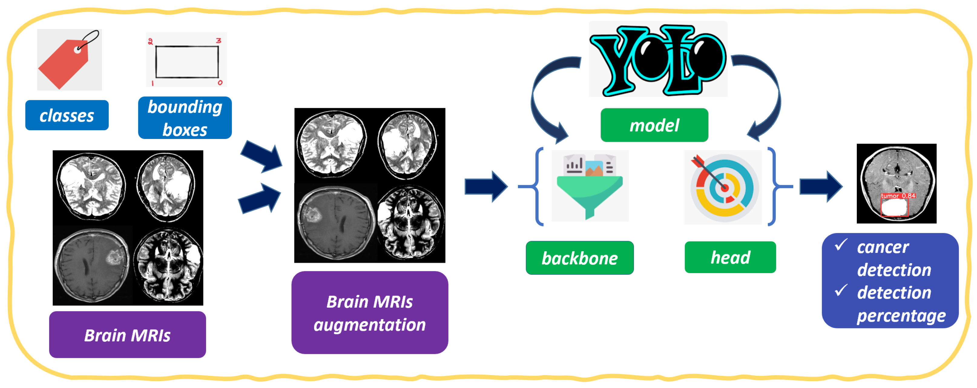
Figure 1. The workflow of the proposed method for brain cancer detection and localization.
Applsci 13 09158 g001
Figure 2. An example of brain MRI.
Applsci 13 09158 g002
Figure 3. The experimental analysis results.
Applsci 13 09158 g003
Figure 4. The precision–recall graph.
Applsci 13 09158 g004
Figure 5. Normalized confusion matrix.
Applsci 13 09158 g005
Figure 6. Sixteen examples of brain images with the related label provided by radiologists, designed to confirm the cancer localization.
Applsci 13 09158 g006
Figure 7. The sixteen images once processed by the proposed model: it is possible to note the red bounding boxes, automatically added by the proposed model, related to the cancerous area. Moreover, for each bounding box, there is the detail about the prediction percentage.
Applsci 13 09158 g007
Table 1. The architecture of the YOLOv8s model for object detection.
LayerFromnParamsModuleArguments
0−11928modules.Conv[3, 32, 3, 2]
1−1118,560modules.Conv[32, 64, 3, 2]
2−1129,056modules.C2f[64, 64, 1, True]
3−1173,984modules.Conv[64, 128, 3, 2]
4−12197,632modules.C2f[128, 128, 2, True]
5−11295,424modules.Conv[128, 256, 3, 2]
6−12788,480modules.C2f[256, 256, 2, True]
7−111,180,672modules.Conv[256, 512, 3, 2]
8−111,838,080modules.C2f[512, 512, 1, True]
9−11656,896modules.SPPF[512, 512, 5]
10−110upsampling.Upsample[None, 2, ‘nearest’]
11[−1, 6]10modules.Concat[1]
12−11591,360modules.C2f[768, 256, 1]
13−110upsampling.Upsample[None, 2, ‘nearest’]
14[−1, 4]10modules.Concat[1]
15−11148,224modules.C2f[384, 128, 1]
16−11147,712modules.Conv[128, 128, 3, 2]
17[−1, 12]10modules.Concat[1]
18−11493,056modules.C2f[384, 256, 1]
19−11590,336modules.Con[256, 256, 3, 2]
20[−1, 9]10modules.Concat[1]
21−111,969,152modules.C2f[768, 512, 1]
22[15, 18, 21]12,116,822modules.Detect[2, [128, 256, 512]]
Table 2. Classification results.
StepImageLabelsPrecisionRecallSpecificitymAP_0.5mAP_0.5:0.95
Training60590.9480.9260.9310.9350.388
Testing60590.9430.9320.9380.9410.421
Disclaimer/Publisher’s Note: The statements, opinions and data contained in all publications are solely those of the individual author(s) and contributor(s) and not of MDPI and/or the editor(s). MDPI and/or the editor(s) disclaim responsibility for any injury to people or property resulting from any ideas, methods, instructions or products referred to in the content.