Planar Delaunay Mesh Smoothing Method Based on Angle and a Deep Q-Network

Abstract

Mesh quality is critical to the accuracy and efficiency of finite element calculations, and mesh smoothing is an essential means of reducing the number of poor elements and improving mesh quality. The deep Q-network-based optimization algorithm for planar Delaunay mesh (unconstrained DQN) has attracted increasing attention due to its advantages in autonomous optimization. However, the unconstrained DQN model does not constrain the movement area of the central node during the training process, and element quality easily falls into a local optimum, resulting in a low generalization of the DQN model. In this paper, an updateable iterative inner polygon is proposed as a constraint to limit the central node’s movement and control the element’s angle. Next, the performance of different neural networks when training the same dataset is analyzed, and the appropriate neural network is selected. After that, the effectiveness and generalization of the method were analyzed. Finally, the results were compared with those obtained by existing methods. The results show that the proposed algorithm can improve the minimum angle of global elements and the shape of poor elements, and the trained DQN model has a high generalization.

1. Introduction

Numerical mesh generation is a preprocessing step in finite element analysis. Mesh generation is the basis of finite element calculations, and high-quality meshes are critical to the results of finite element calculations [1]. Delaunay triangulation is one of the most general automatic finite element mesh generation methods [2]. Due to the influence of internal node insertion, boundary constraints, element size transition, and other factors, the initial mesh formed using the Delaunay triangulation algorithm will have poor elements in local areas. These poor elements will affect the accuracy and efficiency of the finite element calculation [3]. For example, larger element angles lead to larger gradient errors, while smaller angles significantly increase the stiffness matrix condition [4,5], which reduces the solution accuracy and convergence of the iterative solvers. Thus, mesh smoothing is required to improve mesh quality after finite element mesh generation [6].

The optimization methods of a finite element mesh can be divided into topology optimization [7] and geometric optimization according to whether the topology changes in the optimization process. Geometric optimization is also called smoothing; compared with topology optimization, geometric optimization does not change the mesh topology. Laplacian smoothing [8,9,10,11,12,13] is the simplest method, so it is often used. However, using too many iterations of Laplacian smoothing will cause excessive smoothing and reduce the mesh quality. Researchers have proposed an angle-based smoothing method to overcome the shortcomings of Laplacian smoothing [14,15]. This method neglects the selection of the optimal central node coordinates, resulting in an insufficient mesh quality distribution concentration. The optimization-based smoothing method uses some quality metrics to define the cost function, and moving the mesh nodes minimizes or maximizes the cost function. Standard optimization methods include the steepest descent method [16,17], conjugate gradient method [18,19], Newton method [20,21], and downhill simplex method [22]. Optimal Delaunay triangulation (ODT) [23] and centroid Voronoi tessellation (CVT) [24] are two widely used mesh smoothing algorithms based on optimization. This kind of method can achieve a higher-quality mesh optimization, but it has higher computational complexity. The computational cost of mesh smoothing based on optimization is much higher than that of Laplacian smoothing [13].

With the development of artificial intelligence, researchers have begun to explore the application of neural networks and reinforcement learning to mesh generation and smoothing. Ref. [25] proposed a smoothing method based on a neural network. Although this method can improve the average quality of a mesh, it will reduce the minimum mesh quality. Ref. [26] used a deep neural network to predict the optimal locations of nodes. This method can improve the mesh quality but requires tens of thousands of samples with labels, and the training costs are high. Ref. [27] proposed a mesh smoothing method based on a deep Q-network (unconstrained DQN). This method does not limit the active area of the central node. When the central node is close to the polygon boundary, it does not improve the element quality. Through the analysis in Section 4.2 and Section 4.3, we found that the generalization performance of the DQN model trained using this method was low, and it did not have a good optimization effect on meshes that have not participated in the training. The generalization performance is an important characteristic of the DQN model, which determines whether the DQN model has universally applicable properties when dealing with problems in this field.

This paper proposes a planar Delaunay mesh smoothing method based on angle and a deep Q-network. The novelty of this article lies in extracting the inner polygon, polygon, and central node into the features of the mesh, normalizing the features and inputting them into the neural network, and improving the generalization performance of the DQN model [27] through the constructed inner polygon; the minimum angle is also better controlled. Furthermore, an iterative update of the inner polygon is proposed to limit the movement of the central node as a basis for the reward function during neural network training.

The remaining part of this paper is organized as follows: Section 2 presents the unconstrained deep Q-network smoothing method, proposes a method for constructing the inner polygon, and describes the algorithm flow for each stage after adding the inner polygon. Section 3 presents the quality metrics selected in the program and explains the characteristics of polygons composed of triangular elements in the dataset and which neural network structure was used for training the dataset. The effectiveness and generalization of the DQN model trained using the proposed method are analyzed in Section 4. The smoothed results of the proposed method are compared with the smoothed results of existing algorithms, and a finite element analysis is conducted using two examples. In Section 5, our main conclusions and a summary of the main findings of this work are presented, along with a proposal for future research and development of reinforcement learning in the field of mesh optimization.

2. Smoothing Method Based on Angle and Deep Q-Network

2.1. Unconstrained Deep Q-Network Smoothing Method

The unconstrained DQN smoothing method [27] trains polygon datasets with different shapes by exploiting the self-learning ability of the DQN so that agents can find the optimal policy to maximize cumulative rewards. In this method, the central node in the polygon is regarded as the agent, and the polygon is regarded as the moving environment of the agent. The agent takes actions in the environment area, and the action space is selected as four actions on the plane: up, down, left, and right. Each time the agent chooses an action, the state of the environment will change. The state space is the coordinate set of the polygon and central nodes. The node quality is specified as the lowest quality of the triangle element in the polygon. The reward function is set according to three conditions: the change in the quality after the action is taken, the agent moving out of the polygon, and whether the node quality meets the threshold.

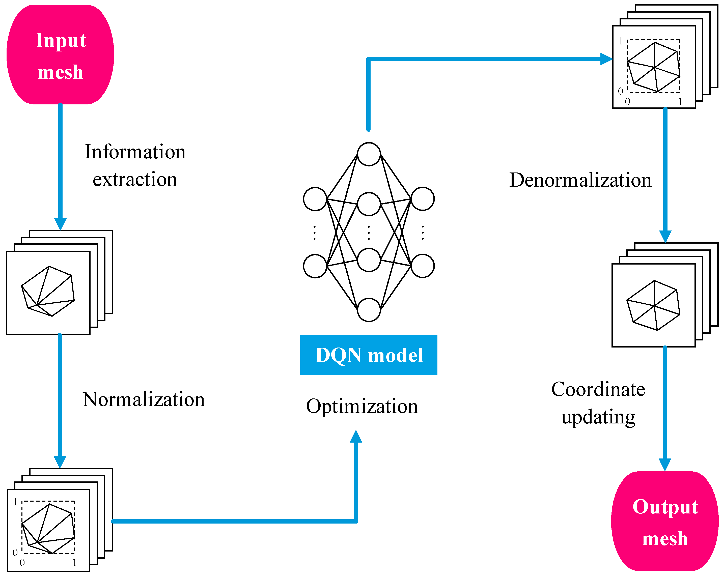
The smoothing process of the unconstrained DQN is shown in Figure 1. Before optimization, the data are normalized and smoothed using the trained DQN model. After the DQN model smooths the mesh, the data need to be denormalized, the coordinates are updated, and finally, the optimized mesh is output.

Figure 1. Flow chart of the unconstrained DQN smoothing method.

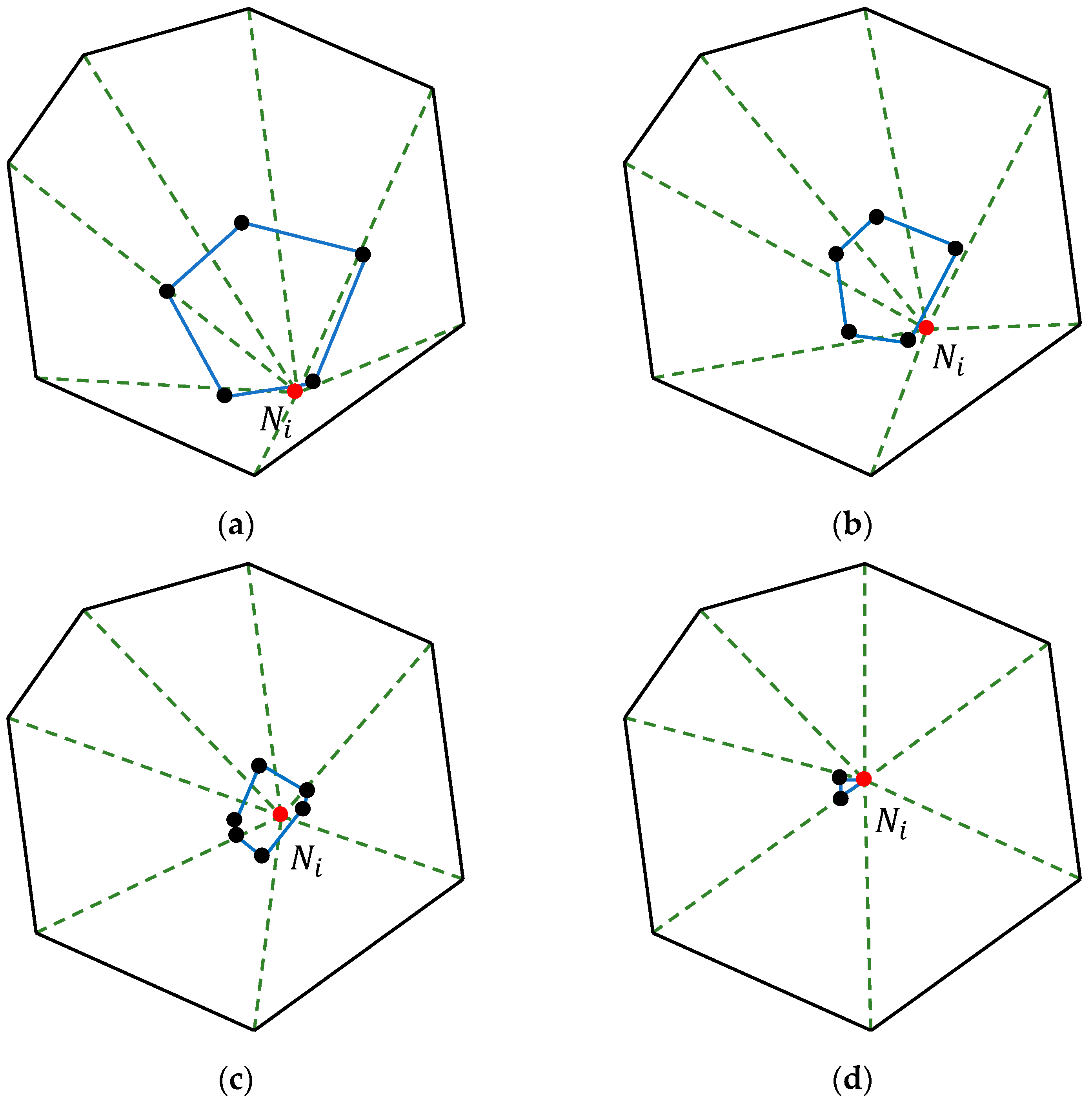
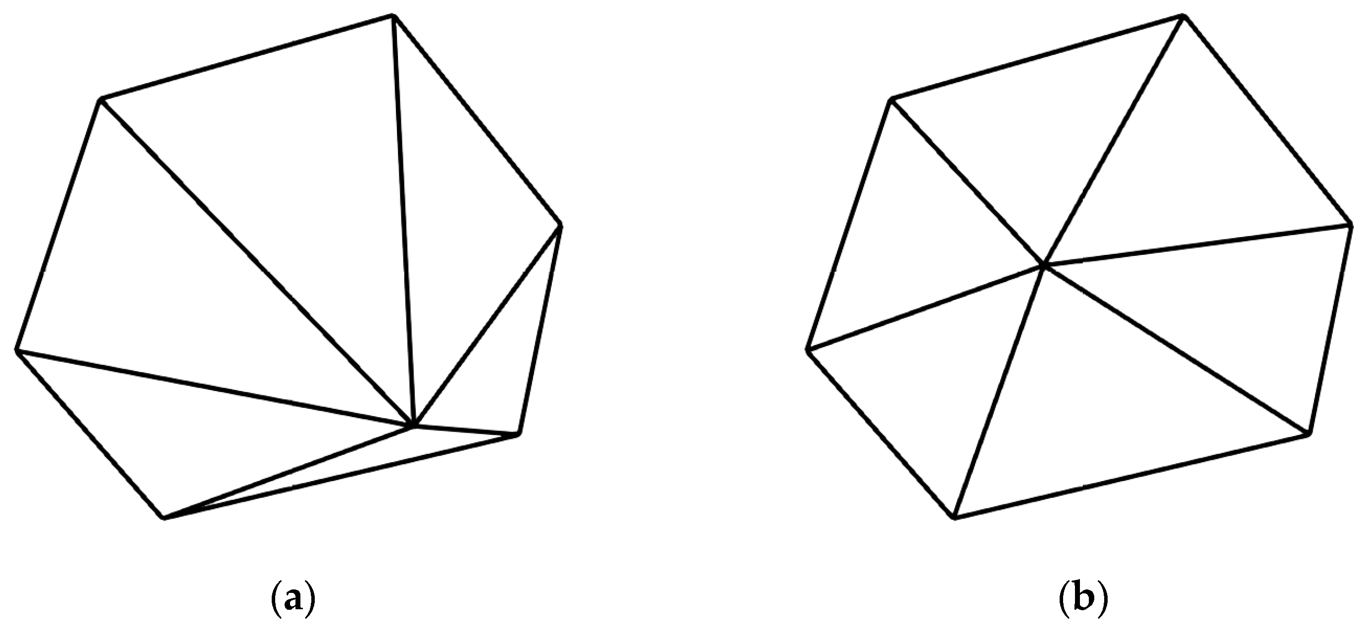
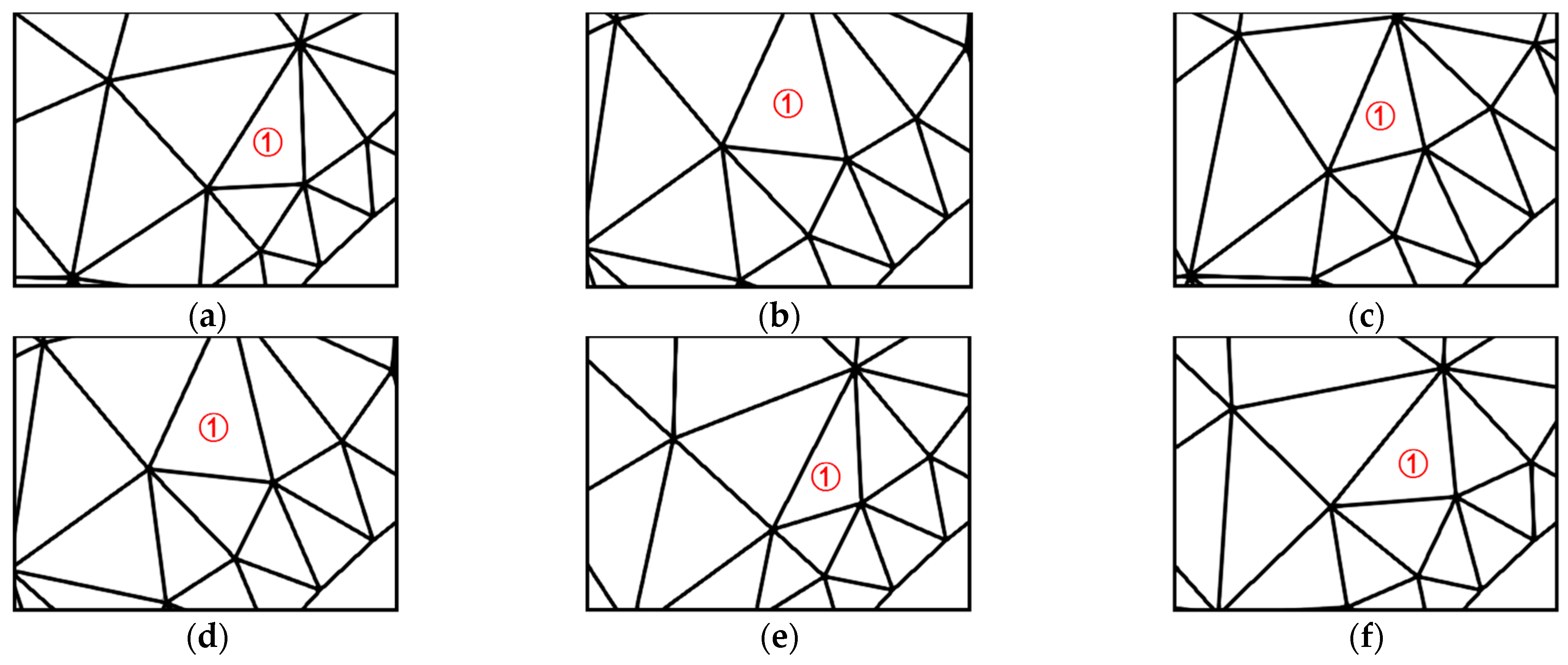
The unconstrained DQN smoothing method does not constrain the moving range of the agent during training. As shown in Figure 2a,b, when the central node moves near the polygon’s boundary, the poor element’s shape is not improved. Because of the exploration rate, the center will try to move to the boundary during training. Such actions do not help improve the quality of nodes. Instead, they consume considerable time for trial and error during training and even make the quality of nodes fall into local optima, leading to difficulties in improving the quality of elements. As shown in Figure 2c,d, when the central node moves in the central area of the polygon, it is helpful to further improve the node quality. Therefore, this paper proposes adding an inner polygon constraint to the polygon’s interior and limiting the central node’s moving range through the iteration during training.

Figure 2. Impact of the central node moving position on node quality. (a) Case 1, where the central node moves near the polygon boundary; (b) Case 1, where the central node moves near the polygon boundary; (c) Case 2, where the central node moves near the center of the polygon; (d) Case 2, where the central node moves near the center of the polygon.

2.2. Construction of the Inner Polygon

The inner polygon is constructed based on the angle-based smoothing method proposed by Zhou and Shimada [14]. As shown in Figure 3a, $N_i$ is the central node of the polygon, and $N_j$ is the adjacent point of the polygon. $\stackrel{\rightharpoonup }{{\mathrm{N}}_j{N}_i}$ denotes $V_j$, $\stackrel{\rightharpoonup }{{\mathrm{N}}_j{N}_{j+1}}$ denotes $V_{j+1}$, and $\stackrel{\rightharpoonup }{{\mathrm{N}}_j{N}_{j-1}}$ denotes $V_{j-1}$. ${\alpha }_1$ is the angle formed by $V_j$, and $V_{j-1}$, and ${\alpha }_2$ are the angles formed by $V_j$ and $V_{j+1}$. With $N_j$ as the center and $\overline{N_i{N}_j}$ as the radius, $V_j$ is rotated until the included angle formed by $V_j$ and $V_{j-1}$ equals to that formed by $V_j$ and $V_{j+1}$. The angle to be rotated is ${\beta }_j$, and the updated central node is shown in Figure 3b. The central node has a total of $k$ adjacent points, so when the same operation is performed $k$ times, $k$ central nodes are generated inside the polygon after one round of the operation, as shown in Figure 3c.

Figure 3. The construction process of the inner polygon. (a) The initial state of a polygon; (b) rotation angle and updated central node; (c) updated scatters; (d) convex hull processing for scattered points falling inside the polygon; and (e) the inner polygon constructed.

Ref. [14] used the mean coordinate value of the updated $k$ central nodes as the new central node. When the updated central node is moved out of the polygon, such nodes will impact the location of the central node, resulting in a reduction in the quality of the element. The updated center point will be referred to as a scatter point in the following text.

In this paper, the updated k scatter points are further processed. First, when the shape of the polygon is too complex or the central node is too close to the boundary, the updated scatter point may fall outside the polygon. Suppose the number of scatter points falling outside the polygon is $m_1$ and the number of scatter points inside the polygon is $m_2$. Then, $m_2=k-m_1$, and these $m_1$ scatter points need to be deleted when constructing the inner polygon. After that, the convex hull algorithm [28] connects $m_2$ scatter points inside the polygon to form an inner polygon. As shown in Figure 3d, suppose the number of points on the convex packet is $v_2$, and the number of points inside the polygon and not on the convex packet is $v_1$. Then, $v_1=m_2-v_2$. Finally, the generated inner polygon is shown in Figure 3e.

2.3. Workflow of the Algorithm

2.3.1. Overview

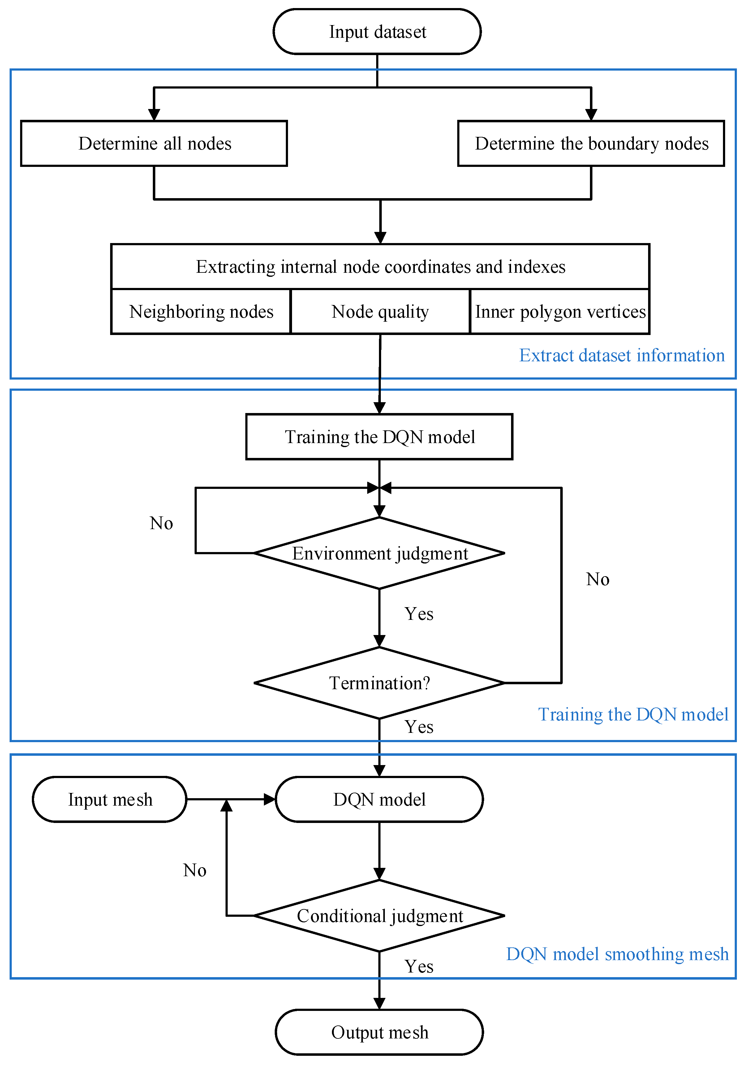
In this paper, we propose a planar Delaunay mesh smoothing algorithm based on angle and a deep Q-network, which is obtained by constructing an inner polygon based on the mesh smoothing method of a deep Q-network, and the algorithm consists of three main steps. (1) The first step is to extract the coordinates of all nodes in the planar mesh dataset. The extracted points include the central, neighboring, and inner polygon nodes. (2) The second step is to determine the information of the dataset, train the features using the deep Q-network, add the features of the inner polygon as constraints, and output the constrained DQN model after the training is completed. (3) The third step is to smooth the mesh according to the policy of constraining the DQN model. Each smoothing requires resetting the points that have been moved out of the inner polygon to the centroid of the inner polygon and continuing to smooth them according to the policy in the model.

The entire workflow of the proposed algorithm is illustrated in Figure 4.

Figure 4. Workflow of the proposed angle and a deep Q-network-based mesh smoothing.

2.3.2. Step 1: Extracting Feature Information from the Dataset

The shortcomings of the deep Q-network-based mesh smoothing algorithm are described in detail in Section 2.1. The DQN model trained using this algorithm does not have good generalization performance when performing mesh smoothing. Based on this algorithm, we propose an improved mesh smoothing method to construct an inner polygon that puts constraints on the agent’s movement. The feature information of the dataset needs to be extracted before training the constrained DQN model, and the specific implementation procedures are as follows:

• Read the boundary nodes and all nodes of the continuum from the dataset and make the difference set between them to get the internal points of the continuum;
• Traverse the internal points and calculate the quality of all triangular elements containing the point, taking the lowest quality as the node quality. Store all node qualities in an array and sort them in ascending order;
• Traverse the interior points, bisect the interior angles of the polygon, and calculate. The scatter coordinates are the updated centroids. Convex the scattered points to get the inner polygon;
• Store the index, node coordinates, node quality, neighboring node index, neighboring node coordinates, and inner polygon vertex coordinates of all internal points in memory.

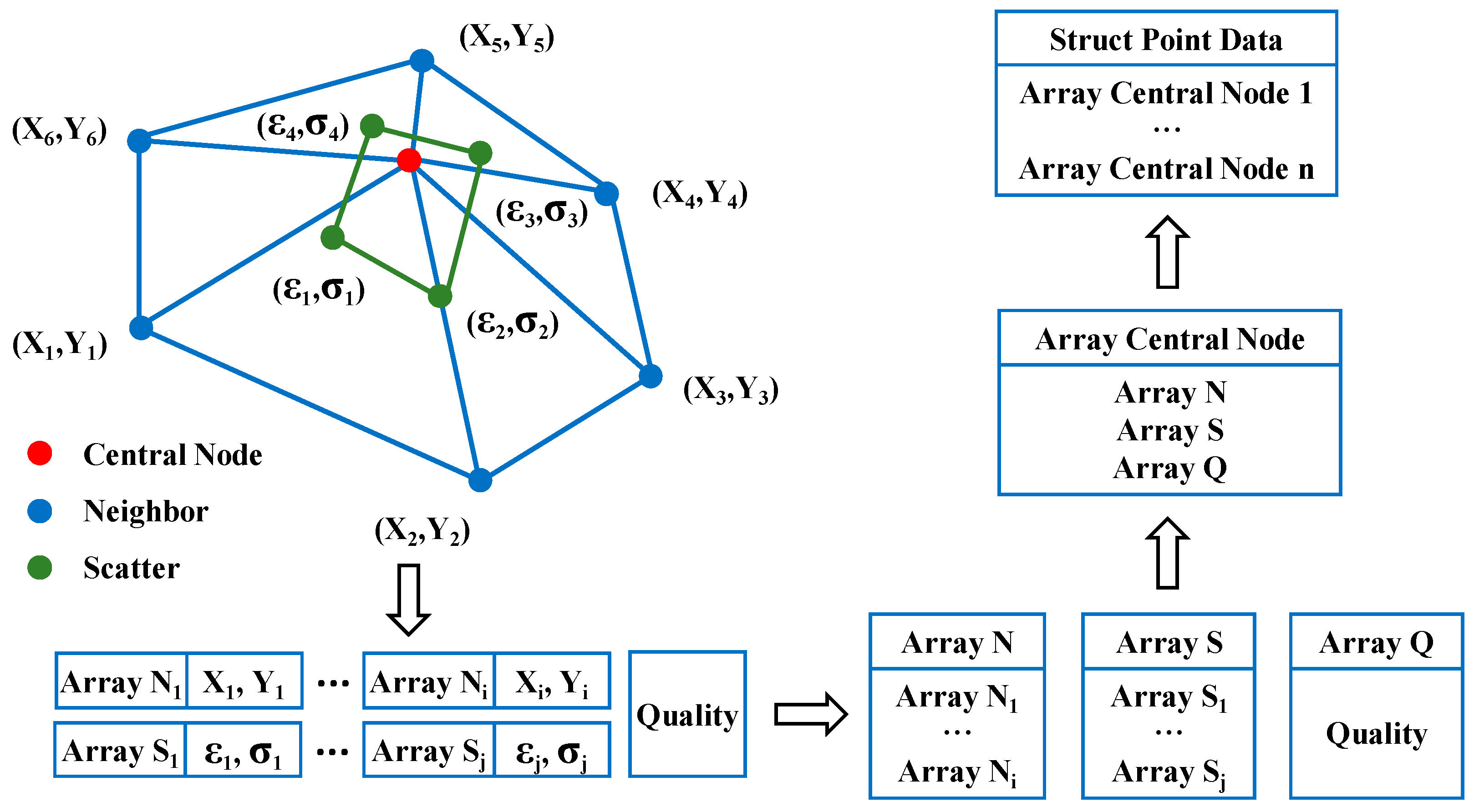
The information of all nodes in the dataset can be extracted using the above method. We store the node information of all internal points in memory to facilitate subsequent extraction of data features for input in the neural network for training. Figure 5 briefly illustrates the data structure of the extracted information.

Figure 5. The data structure of mesh data information.

2.3.3. Step 2: Training of DQN Model

In this paper, the reinforcement learning model with inner polygon constraints is designed as follows, with a design reference to Zhang [27].

Agent: the central node of the polygon.

Environment: polygon and inner polygon.

Action vector: action = {up, down, left, right}, move step reference to Gong [16], take $Move\_step=0.02·l_{min}$, where $l_{min}$ is the shortest side length of the polygon.

State vector: $State=\left\{{\delta }_c,{\delta }_1, \cdots , {\delta }_k,{\theta }_1, \cdots , {\theta }_{v_2}\right\}$, where ${\delta }_c$ is the coordinate of the agent, ${\delta }_k$ is the vertex coordinate of the polygon, $k$ is the number of polygon nodes, ${\theta }_{v_2}$ is the vertex coordinate of the inner polygon, and $v_2$ is the number of inner polygon nodes.

Reward function: According to the design in [27], a new function is designed, as shown in Table 1. In the new reward function, a weak penalty is applied when the intelligence moves out of the inner polygon, and a strong penalty is applied when it moves out of the polygon.

Table 1. Reward function setting for DQN model.

State	Reward Function
Normal	$\left(q_{v,t}-q_{v,t-1}\right)\times 100$
Node quality exceeds the threshold	10
The agent moves out of the inner polygon	−10
The agent moves out of the polygon	−100

We set the hyperparameter learning rate to four levels: 0.1, 0.01, 0.0001, and 0.0001. The training results show that when the learning rate is 0.01, the learning efficiency and quality are relatively balanced, and the mesh optimization effect is optimal. During the training process, the agent adopts the Epsilon-Greedy algorithm. The epsilon is 0.9, which means that the agent has a 90% probability of randomly taking action during the training process and a 10% probability of taking action based on the maximum Q value. The remaining hyperparameters are set regarding Zhang [27]. The parameter settings of the neural network are shown in Table 2.

Table 2. Table of parameter setting for neural networks.

Parameter	Symbol	Value
learning rate	$\mathsf{\alpha }$	0.01
decay rate	$\mathsf{\gamma }$	0.9
epsilon	$\mathsf{\epsilon }$	0.9
number of times experience pool D starts to replay	$\mathrm{N}$	500
batch size	$\mathrm{m}$	32
number of intervals for updating objective function	$\mathrm{C}$	300
maximum number of steps in a single round	$\mathrm{T}$	200
maximum number of rounds	$\mathrm{M}$	1000
optimizer	RMSProp
activation function	ReLU

Neural networks act as actuators in deep reinforcement learning to compute and store Q-values. The agent observes the state and takes action, and the state of the environment is updated to the next moment. The environment feeds the agent with a reward based on the node quality and constraints at the next moment. The agent recalculates the Q-value based on the state and reward of the current moment and the delayed moment. The agent iterates the above steps during training to find the optimal policy that maximizes the cumulative Q-value. The DQN model is saved at the end of the training, and the update process of the neural network parameter θ is as follows:

Input: state vector S, action vector A, learning rate α, decay rate γ, epsilon ε, current Q-network Q, target Q-network Q ‘, batch size m, maximum round M, maximum step T, and update frequency C of the target Q-network.

Output: parameters θ of the current Q-network.

• The program reads the information about the dataset stored in memory. Normalize the dataset features by scaling the polygon to be within a square region with a side length of 1;
• Initialize experience playback pool D, randomly initialize the parameters of the real Q-network θ, and initialize the parameters θ′ of the target Q-network equal to θ;
• The program reads the state vector of the dataset and obtains the eigenvector $\Phi \left(S_t\right)$. Using $\Phi \left(S_t\right)$ as the input in the Q-network, calculate the Q-values corresponding to all actions. ε—the greedy algorithm selects the corresponding action from the current Q-value. The agent has a probability of 0.9 to randomly select actions to search for other strategies to maximize rewards and benefits. There is a 10% probability of selecting the action corresponding to the maximum Q-value;
• Execute action $A_t$ in the current state $S_t$, to obtain the feature vector corresponding to the next state $\Phi \left(S_{t+1}\right)$, reward $R_t$, and terminate status conducted;

  4.1.

  Calculate the node quality $q_{v,t-1}$ and $q_{v,t}$ before and after the agent moves and set the reward value to $\left(q_{v,t}-q_{v,t-1}\right)\times 100$;

  4.2.

  Determine whether the current node quality meets the quality threshold. If it does, terminate this round of training and start a new round;

  4.3.

  Determine whether the intelligent agent has moved out of the inner polygon. If so, give a reward of −10 and continue training;

  4.4.

  Determine whether the agent has moved out of the polygon. If so, give a reward of −100 and terminate this round of training. Otherwise, continue;

• Store $\left\{S_t, A_t,R_t,S_{t+1}\right\}$ as an array, and store the array in the experience playback pool. Update status $S_t$ to $S_{t+1}$;
• Randomly sample m samples $\left\{S_j, A_j,R_j,S_{j+1}\right\}$ from the experience playback pool D, where j = 1, 2,…, m. Calculate the current target Q-value $y_j$ using the following Equation;

  $$y_j=\{\begin{array}{c}{R}_j , don{e}_j is True\\ R_j+\gamma \max Q^{\prime }\left(S_{j+1}, A_{j+1},{\theta }^{\prime }\right), don{e}_j is False\end{array}$$

  (1)
• Perform a gradient descent on ${\left(y_j-Q\left(S_j, A_j, \theta \right)\right)}^2$ to update the parameters θ of the real Q-network.
• Update the parameters ${\theta }^{\prime }$ of the target Q-network every C step. The round ends when the number of steps the agent moves reaches the maximum number of steps, T.
• Training is stopped when the maximum number of training rounds, M, is reached and the data features are denormalized. Otherwise, it goes to Step 3;

The reward is calculated with the node quality before and after the agent’s movement during training, and the quality threshold is used as the optimization target. Training is performed in order of node quality from lowest to highest. This setup facilitates the agent to train the policy of improving the minimum quality as the highest priority. After the neural network parameter $\theta$ is updated, the node’s movement policy can be determined through Equation (2).

$${\pi }^{*}=\arg \max Q(S,A,\theta )$$

(2)

For the algorithm to converge well, the epsilon $\epsilon$ musts to be reduced by 0.1 as the iteration progresses. After the training, we can get the constrained DQN model with the smoothing capability of the mesh.

2.3.4. Step 3: Constrain DQN Model for Mesh Smoothing

The constrained DQN model guides the agent to move within the polygon based on the optimal policy. The stored DQN models are named using the number of features because of the difference in the number of features. The program reads the mesh data and selects the corresponding DQN model for optimization according to the number of polygon features contained. The inner polygon is used as a weak constraint in the optimization process, and when the agent moves out of the inner polygon, the coordinates of the agent are reset to the mean value of the coordinates of the nodes of the inner polygon, and the DQN model continues to guide the agent to move. The DQN model takes the improvement of node quality as the optimization objective and optimizes the low-quality nodes first in the optimization process according to the optimal policy. After each iteration, the lowest node quality increases and the highest node quality reaches the threshold, and the overall number of nodes that do not satisfy the threshold decreases.

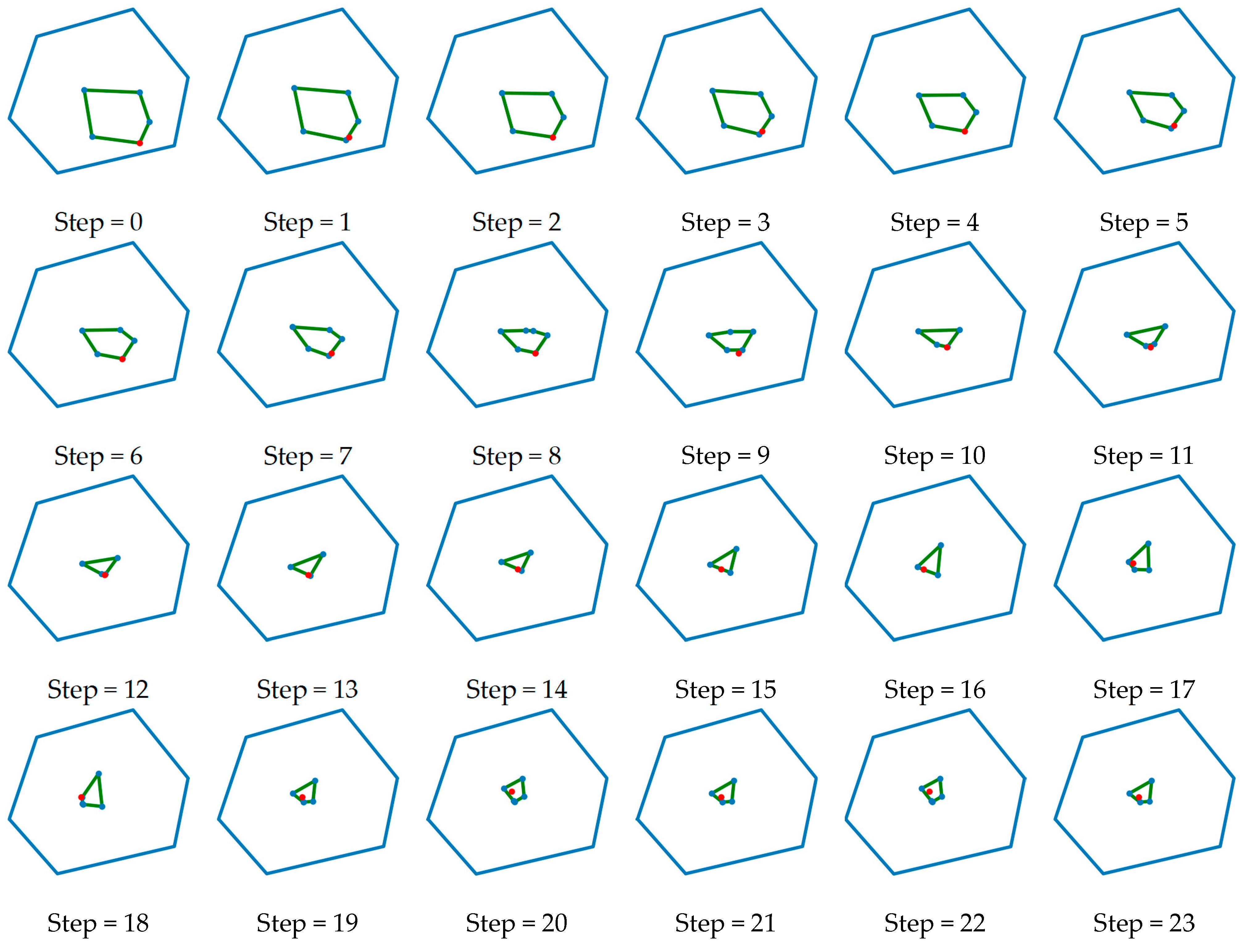
The size and position of the inner polygon change constantly during the smoothing process. As shown in Figure 6, when the node quality is low, the area formed by the inner polygon is large and close to the polygon boundary. As the number of iterations increases, the quality of nodes improves, the area formed by the inner polygon starts to shrink, and the position moves to the central area. When the node quality is high, the position of the inner polygon is close to the center of the polygon. The central node finally moves in the center area to improve the node quality.

Figure 6. Changes in the size and position of the inner polygon. (a) The inner polygon when the center node is close to the polygon boundary; (b) The inner polygon when the central node moves towards the central region; (c) The inner polygon when the central node is close to the central region; (d) The inner polygon when the center node is located at the centroid of the polygon.

3. Parameter Setting and Data Preparation of the Constrained DQN Model

3.1. Quality Metric

In the program, the aspect ratio [25] of the triangle is used as the quality metric, and the formula is as follows:

$$q_e=\frac{4\sqrt{3}·S}{l_1^2+l_2^2+l_3^2}$$

(3)

where $l_i$ is the side length of the triangle, and S is the area of the triangle. Here, $q_e\in \left[0,1\right]$, and the closer the numerical value is to 0, the worse the mesh quality (conversely, the closer the numerical value is to 1, the better the mesh quality).

In the data statistics, the aspect ratio and maximum/minimum angle are used to evaluate the mesh quality, reflecting the optimization effect of the constrained DQN on poor element angles. Ref. [5] showed that the stiffness matrix condition depends on the element’s shape, and elements with small angles will lead to poor matrix conditions, proving that the minimum angle can be used as an index to evaluate the mesh quality.

3.2. Dataset Preparation

Considering that the number of neighboring nodes of free nodes is not unique, we train different models for different types of polygons in this paper, including nodes 3, 4, 5, 6, 7, 8, and 9. Different types of polygons are shown in Figure 7. Polygons with nodes 5, 6, and 7 are common in triangular meshes, while polygons with nodes 3, 4, 8, and 9 are rare. This paper sets 40 finite element mesh models as the dataset. There are mesh models with the same number of nodes in the dataset, but their mesh quality differs. This data enhancement method is used to ensure the generalization performance of the DQN model.

Figure 7. Different types of polygons. (a) k = 3; (b) k = 4; (c) k = 5; (d) k = 6; (e) k = 7; (f) k = 8; (g) k = 9.

Before training the DQN model, the dataset needs to be normalized [25]. After data normalization, the state space scale of the model design can be guaranteed to be the same, and the training efficiency of the DQN model can be improved. After mesh smoothing is completed, the coordinates need to be mapped back to the global coordinate system, which is called data denormalization.

3.3. Neural Network and Network Parameter Setting

The structure of the Q-network changes depending on the number of hidden layers and the number of neural units. In this paper, we set the number of hidden layers to one and two, and the number of neural units with one hidden layer is 10, 20, 30, 40, 50, and 60. Q-networks with two hidden layers are set with the same number of neural units in the hidden layers and fully connected between the two hidden layers. Q-networks with different structures are used to train the dataset. The numerical convergence of the average Q-value and the average reward with the number of training rounds is output after the training is completed. The convergence using different Q-networks for training is shown in Figure 8.

Figure 8. Neural network performance analysis chart. (a) The growth curve of average Q-value with training epochs; (b) the growth curve of average reward with training epochs.

Figure 8a shows the variation of the average Q-values of different Q-networks as the number of training epochs increases. The average Q-value of the Q-network with one hidden layer and 20 neural units grows more slowly when the number of training epochs is 0–5; it grows rapidly when the number of training epochs is 5–10. It grows slowly when the number of training epochs is 10–15; after 15 epochs, it stays around 39.174, and the average Q-value changes more smoothly compared with other Q-networks. Figure 8b shows the variation of the average reward with increasing training epochs using different Q-networks. The Q-network with one hidden layer and 20 neural units has a smooth change in the average reward when compared with other Q-networks at 10–20 training epochs; after 20 epochs, there is a significant decrease in the average reward. Considering the stability of the DQN model, the number of training epochs is set as 16. Since the reward of −100 given by the environment when the agent moves out of the polygon is much smaller than the reward obtained by the improved node quality after the agent moves, the average reward is <0. This is set so that the DQN model does not produce inverted elements when smoothing the mesh. According to the experimental results, such a reward setting is effective and does not negatively affect the performance of the DQN model.

The total number of layers in the neural network is two—the first is hidden, and the second is an output layer. The state space of the dataset is used as the input, and the number of neural units in the input layer is $n_1=2\times \left(1+k+l\right)$, where the central node needs to be recorded as a feature, $k$ is the number of polygon nodes, and $l$ is the number of inner polygon nodes. The number of neural units in the hidden layer is $n_2=20$. The action space of the dataset is taken as the output, and the number of neural units in the output layer is $n_3=4$. The structure of the neural network is shown in Figure 9.

Figure 9. Schematic diagram of neural network structure.

4. Results and Discussion

An Intel Core i7-4710MQ 2.50 GHz CPU with 16 GB of memory and a Windows 10 operating system was used. The constrained DQN model was based on Python, and the neural network framework used TensorFlow 1.15.0. Fewer neural network layers were used, so it ran faster. Forty finite element mesh models were studied, training was performed 16 times, and the total training time was approximately 6 h. The Laplacian, angle-based, ODT, CVT, and unconstrained DQN methods as well as the constrained DQN were used for comparison. The Laplacian, angle-based, ODT, and CVT methods adopt the results after ten iterations. Both unconstrained and constrained DQN models were trained using the same dataset.

4.1. Effectiveness Analysis

Example 1 is a polygon with a central node of one and neighboring nodes of six. The comparison before and after smoothing using the proposed method in Example 1 is shown in Figure 10. From the comparison results, it is clear that the optimization effect of the proposed method is obvious.

Figure 10. Example 1 smoothing front-back diagram. (a) Before smoothing; (b) after smoothing.

As shown in Figure 11, the node quality of Example 1 was stable at 0.92 after the central node moved 20 steps, which proves that the model converges, and the node quality converges to the local optimal position.

Figure 11. Node quality convergence graph.

As shown in Figure 12, it is the convergence of the inner polygon as it moves with the central node. It can be observed that as the quality of the nodes increased, the size of the inner polygon decreased and moved toward the center of the polygon. The polygon within the central node is a weak constraint, moving toward improving the quality of the node, proving that the updated inner polygon helps improve the node’s quality.

Figure 12. Inner polygon convergence graph.

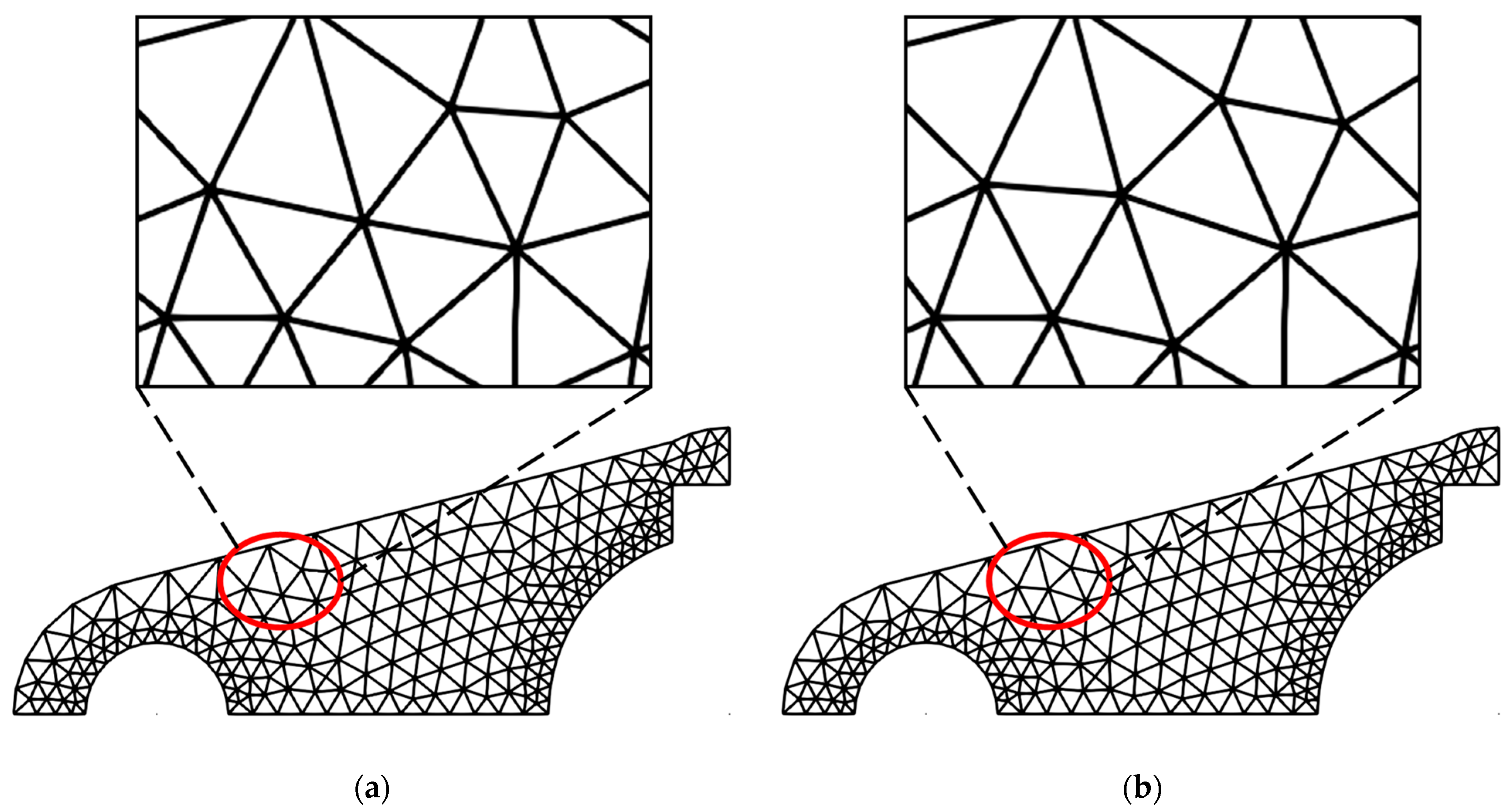
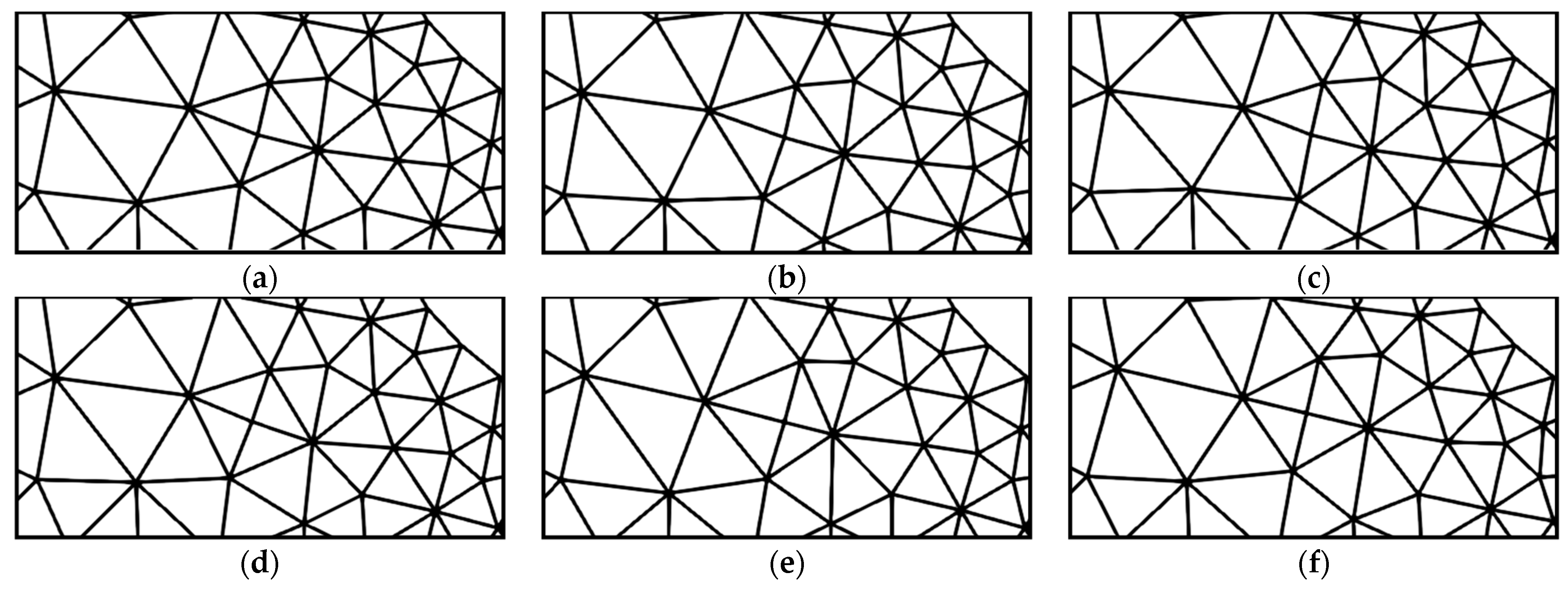
The effectiveness analysis of the proposed method and the node quality convergence analysis were performed for Example 1 above. The following three types of mesh for quarter mechanical components were used to demonstrate the effectiveness of using constrained DQN models for mesh smoothing. As shown in Figure 13, in Example 2, after constrained DQN smoothing, the minimum angle increases, the shape of the poor element is improved, and the optimized mesh is more regular than the initial mesh. Example 3 has many poor elements, as shown in Figure 14. After optimization, the poor elements were eliminated, and the transition effect between elements of different sizes was significantly improved. As shown in Figure 15, the mesh quality of Example 4 is high and has a good mesh size gradient. After smoothing, the angle of the element was improved, and the mesh size gradient was better controlled.

Figure 13. Effectiveness of Example 2 comparison before and after smoothing. (a) Before smoothing; (b) after smoothing.

Figure 14. Effectiveness of Example 3 comparison before and after smoothing. (a) Before smoothing; (b) after smoothing.

Figure 15. Effectiveness of Example 4 comparison before and after smoothing. (a) Before smoothing; (b) after smoothing.

The minimum angle, maximum angle, minimum quality, and average quality before and after smoothing for the above three examples are shown in Table 3. The minimum angle, maximum angle, and minimum quality were significantly improved for all three examples. The average quality of Examples 2 and 3 increased after optimization, but the average quality of example 4 decreased slightly.

Table 3. Table of comparison before and after mesh smoothing.

Mesh	State	Nodes	Min. θ	Max. θ	Min. q	Avg. q
2	Before smoothing	619	18.3706	129.4545	0.4802	0.8632
	After smoothing		34.1760	99.4288	0.7810	0.9279
3	Before smoothing	426	17.8954	128.0146	0.5009	0.7906
	After smoothing		34.9065	93.8188	0.8173	0.9361
4	Before smoothing	426	33.1073	98.6044	0.7962	0.9677
	After smoothing		37.6581	91.6064	0.8517	0.9629

As mentioned above, the constrained DQN model can effectively eliminate poor elements, improve mesh quality and minimum angle of elements, and control the gradient of mesh size when smoothing the mesh.

4.2. Generalization Analysis of Constrained DQN Model

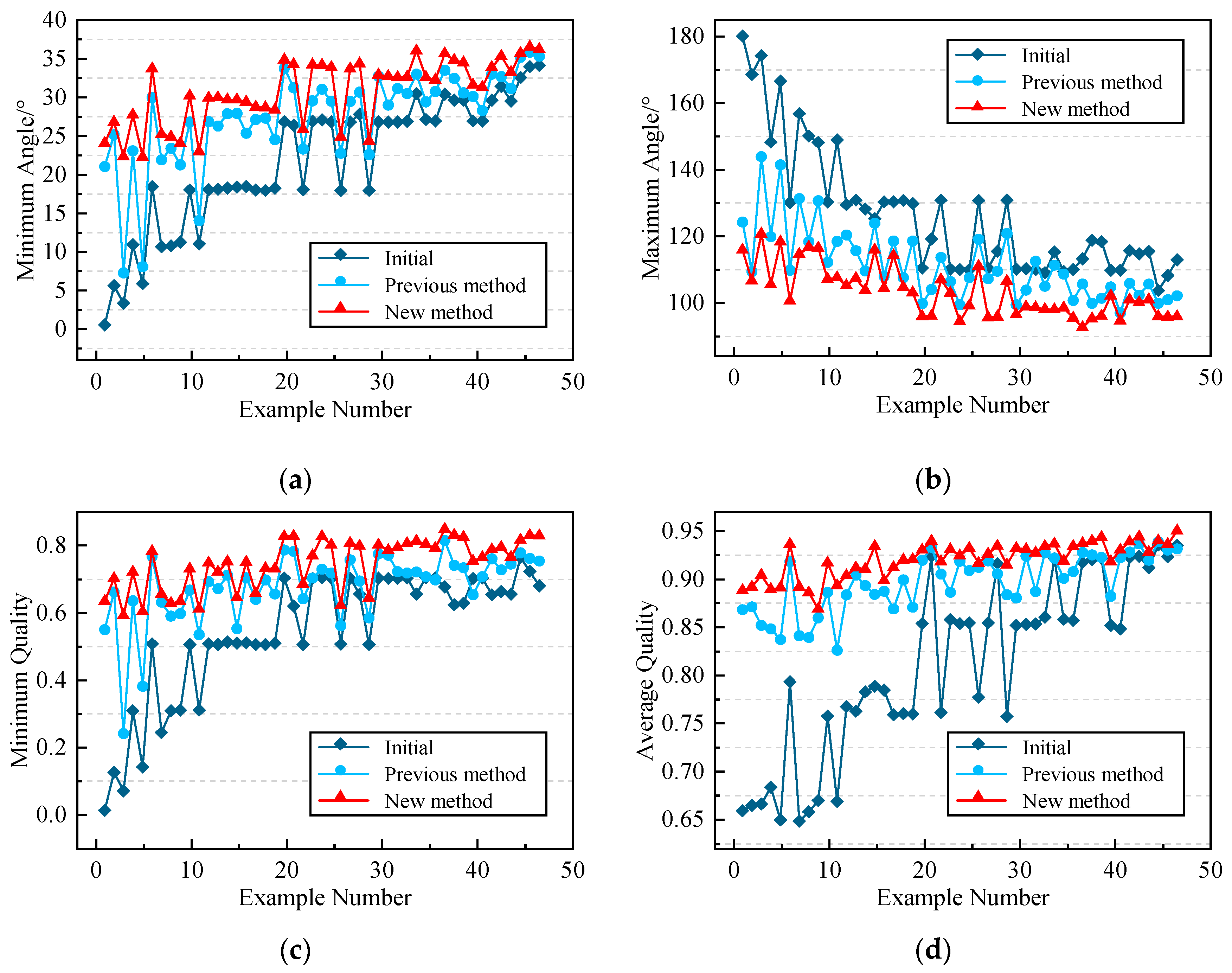
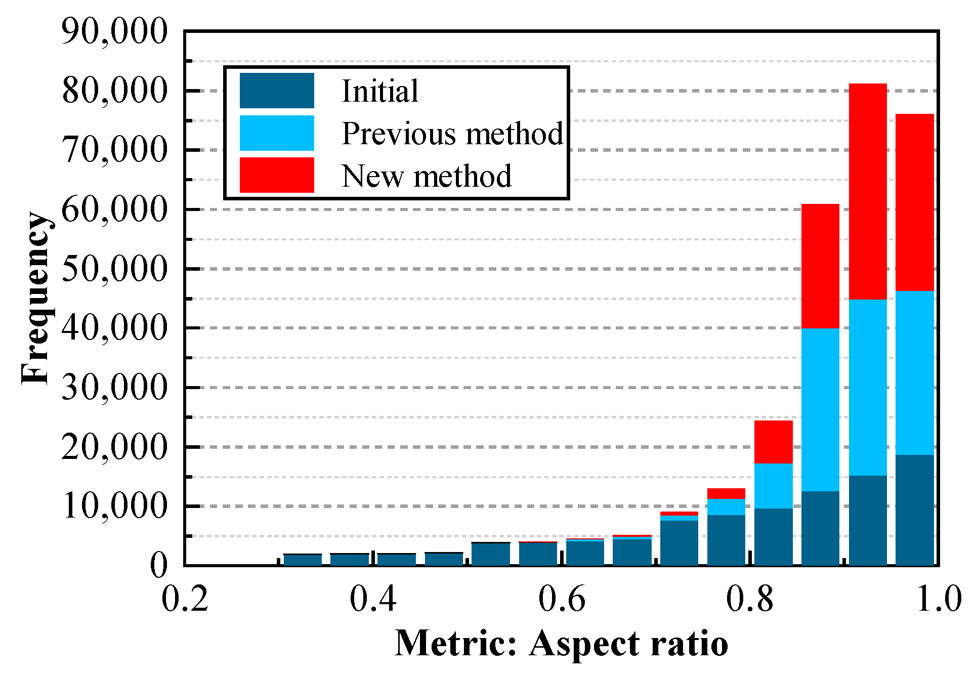
This section used 48 sets of untrained data to compare the generalization ability of the new method and the previous method [27]. Figure 16 shows the minimum angle, maximum angle, minimum quality, and average quality of 48 meshes optimized using previous and new methods. It can be clearly seen that the new method has higher generalization ability and better optimization results compared to the previous methods. As shown in Figure 17, the quality distribution of all elements in 48 sets of mesh data is shown. After optimization with the constrained DQN model, the number of elements with a quality lower than 0.8 was significantly reduced. The distribution of element quality was more concentrated.

Figure 16. Generalizability analysis of constrained DQN models. (a) Minimum angle contrast; (b) maximum angle contrast; (c) minimum quality contrast; (d) and average quality contrast.

Figure 17. Model generalization analysis chart.

In summary, the generalization performance of the constrained DQN model is high and has universal applicability, which can be applied in practical applications.

4.3. Comparative Analysis of Experiments

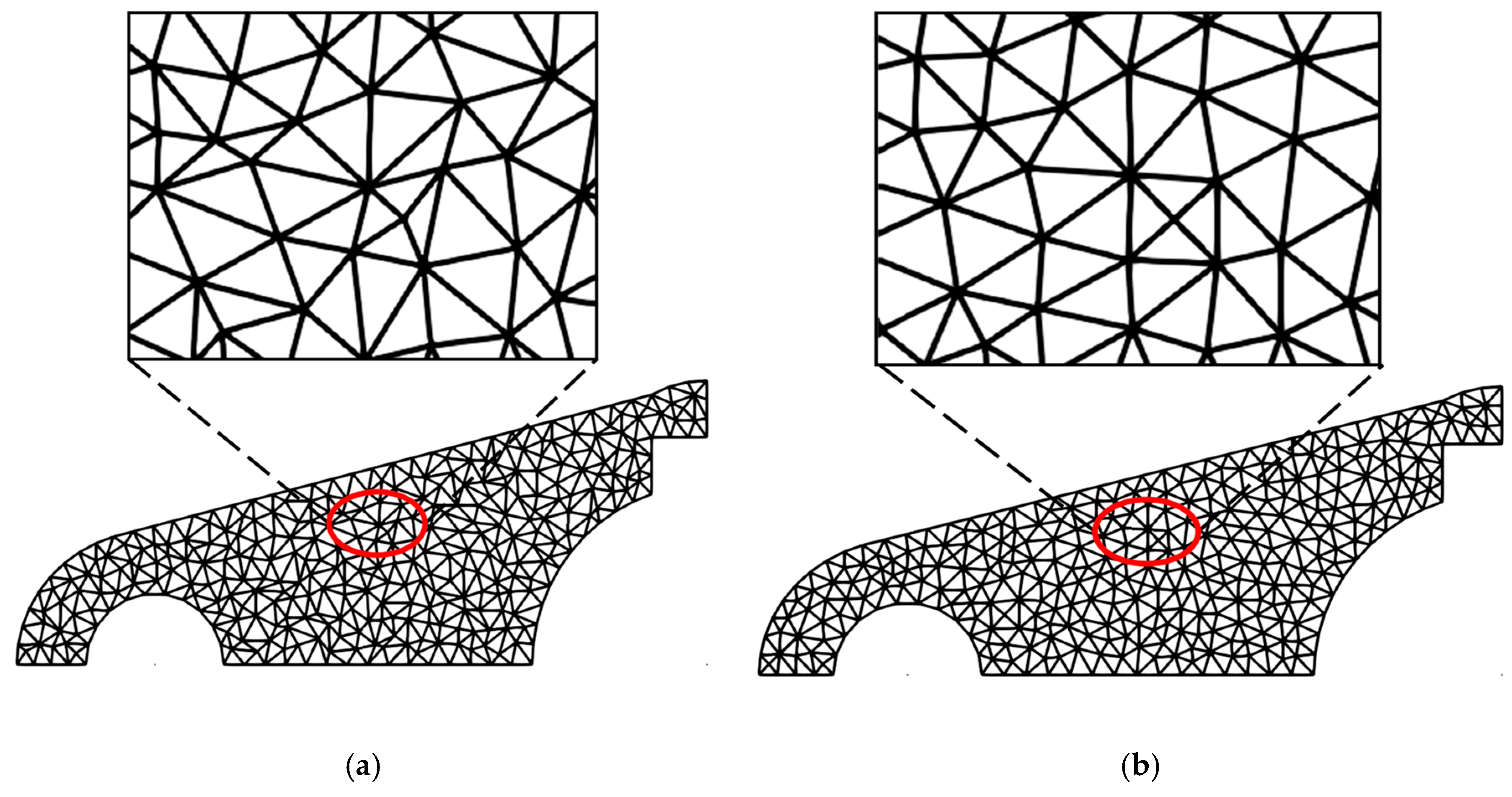
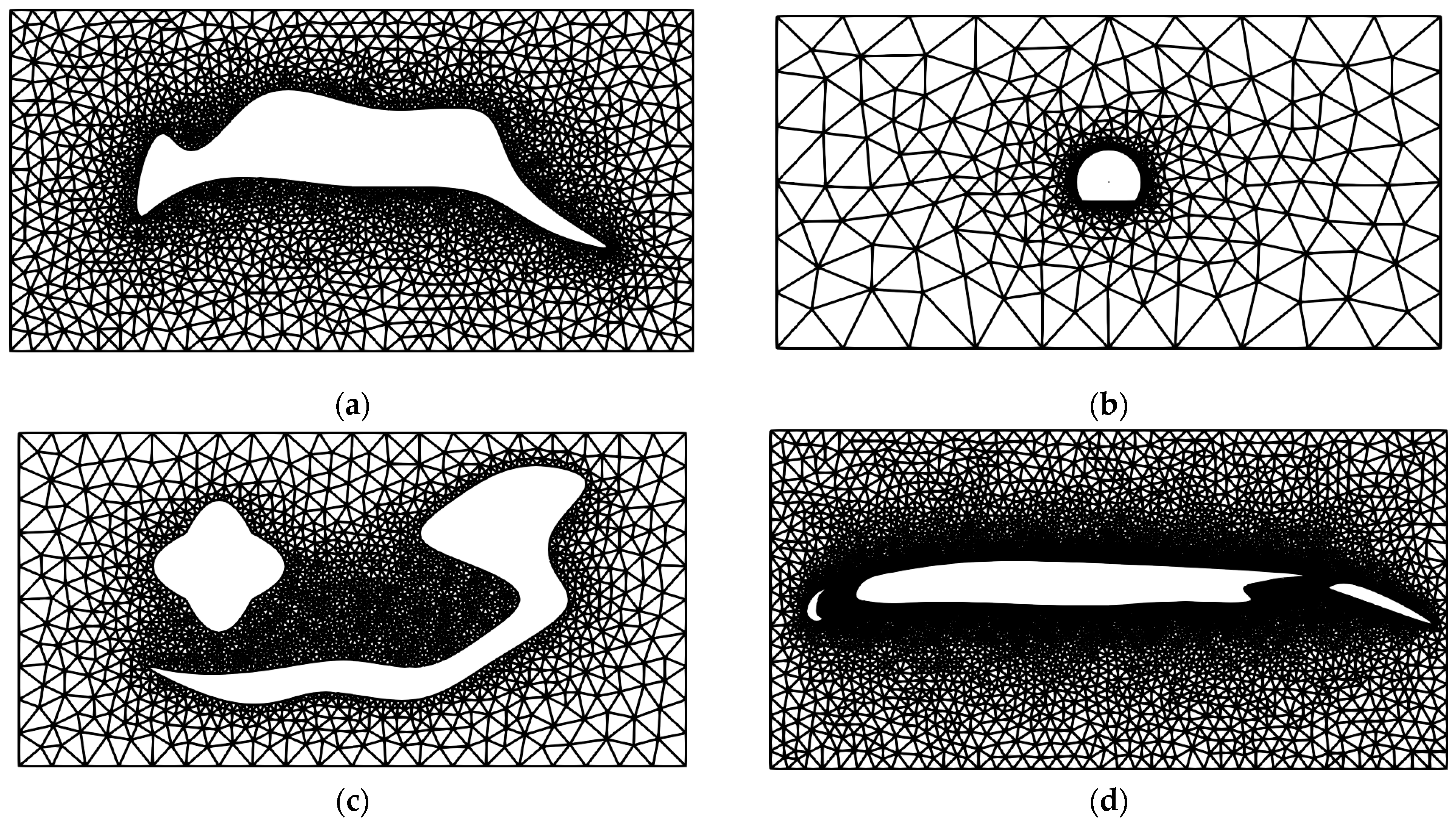
In this section, we use four examples for an experimental comparison analysis, as shown in Figure 18, and the number of nodes are 2027, 926, 2987, and 5115, respectively. The red circle is the location for local comparison in the following text. It should be noted that Example 2 is a mesh in the dataset, while the other three examples have not undergone DQN model training. The results of the four examples after optimization in this paper are shown in Figure 19. Comparing Figure 18 and Figure 19, it can be seen that the proposed method can show good optimization effects in meshes with different element sizes and boundary shapes and can effectively reduce the number of poor elements.

Figure 18. Initial mesh. (a) Example 1; (b) Example 2; (c) Example 3; and (d) Example 4.

Figure 19. The mesh after smoothing using the method in this paper. (a) Example 1; (b) Example 2; (c) Example 3; (d) and Example 4.

In addition, Laplacian [8], angle-based [14], ODT [23], CVT [24], and unconstrained-DQN [27] are used for comparison in this paper. The experimental results are shown in Table 4, where Min. θ is the minimum angle, Max. θ is the maximum angle, (a) is the number of elements with angles less than 30 degrees, (b) is the number of elements with angles greater than 100 degrees, q is the quality of the elements calculated from the aspect ratio, Min. q is the minimum quality, and Avg. q is the average quality. In the following, (a) and (b) are collectively called the number of poor elements.

Table 4. Comparison table of the experimental results.

Mesh	Method	Time/(s)	Nodes	Min. θ	Max. θ	(a)	(b)	Min. q	Avg. q
1	Initial	/		17.62	130.12	1434	1115	0.5001	0.7715
	Laplacian	0.2886		26.86	110.70	3	14	0.6495	0.9608
	Angle-based	0.4520		26.29	105.47	2	7	0.6840	0.9537
	ODT	0.3890	2027	19.00	126.50	42	54	0.5125	0.9109
	CVT	0.3390		27.90	106.34	6	12	0.7249	0.9308
	Unconstrained DQN	1.5944		25.78	114.74	24	37	0.6479	0.9185
	Constrained DQN	1.6218		32.499	96.28	0	0	0.7944	0.9426
2	Initial	/		10.49	146.45	158	117	0.2902	0.8481
	Laplacian	0.1172		28.05	110.21	6	7	0.6713	0.9239
	Angle-based	0.1461		21.67	106.68	28	11	0.5972	0.9096
	ODT	0.1367	926	22.70	124.73	26	30	0.5517	0.9019
	CVT	0.1211		27.14805	114.34	4	12	0.6454	0.9154
	Unconstrained DQN	0.3721		26.05	104.54	2	6	0.6871	0.9179
	Constrained DQN	0.3986		29.25	100.25	1	1	0.7249	0.9208
3	Initial	/		33.31	101.55	0	3	0.7713	0.9499
	Laplacian	0.3666		30.27	102.95	0	8	0.7166	0.9563
	Angle-based	0.7174		25.05	120.23	13	11	0.5888	0.9474
	ODT	0.5078	2987	33.07	101.55	0	2	0.7713	0.9481
	CVT	0.4544		32.15	99.94	0	0	0.7850	0.9492
	Unconstrained DQN	2.2742		34.68	98.56	0	0	0.7978	0.9487
	Constrained DQN	2.3175		36.18	94.92	0	0	0.8229	0.9496
4	Initial	/		17.67	130.17	3789	2908	0.5001	0.7686
	Laplacian	1.1419		26.00	109.88	3	14	0.6560	0.9630
	Angle-based	1.6108		23.23	103.44	16	17	0.6196	0.9560
	ODT	1.5983	5115	19.56	128.79	64	69	0.5041	0.9367
	CVT	1.4202		24.03	105.90	11	24	0.6490	0.9486
	Unconstrained DQN	3.6788		23.97	117.88	29	41	0.6365	0.9127
	Constrained DQN	3.7988		32.31	100.77	0	2	0.7539	0.9465

Note: bold means the best result; (a): number of angles < 30°; (b): number of angles > 100°.

As can be seen from Table 4, Laplacian smoothing has the shortest running time and the highest average quality. Still, it can lead to ineffective element quality improvement due to the geometric shape of some regions. Based on the minimum quality and the number of poor elements of Example 3, it can be found that Laplacian smoothing is prone to over-optimization for higher-quality meshes like Example 3, resulting in an increase in the number of poor elements. The angle-based smoothing method has a significantly higher running time due to the need to calculate the top angle of the polygon and, except for Example 3, provides good control of the maximum angle compared to Laplacian smoothing. The CVT algorithm has less running time than the ODT algorithm; in terms of average quality, the CVT algorithm is slightly better than the ODT algorithm. The ODT algorithm is not significant for the optimization of the maximum angle. Constraint DQN has a longer running time compared to the above methods. However, due to the autonomous learning nature of the agent in reinforcement learning, the number of poor elements can be effectively reduced compared to the other methods mentioned above when optimizing a mesh in a training set like Example 2. In addition, the method fails to produce better optimization results for three examples outside the training set, demonstrating that the generalization ability of the constrained DQN model needs to be improved. The algorithm in this paper has an increased running time relative to the first four methods because it improves the constrained DQN. However, the optimized mesh has the largest minimum angle, the smallest maximum angle, the smallest number of poor elements, and the highest minimum quality compared to the meshes optimized using the other five algorithms. Additionally, the average quality of the four examples optimized with the proposed method has improved compared to the constrained DQN and reached a higher level than other methods. However, since the algorithm in this paper improves the minimum quality significantly, it will be more difficult to improve the average quality again with smoothing.

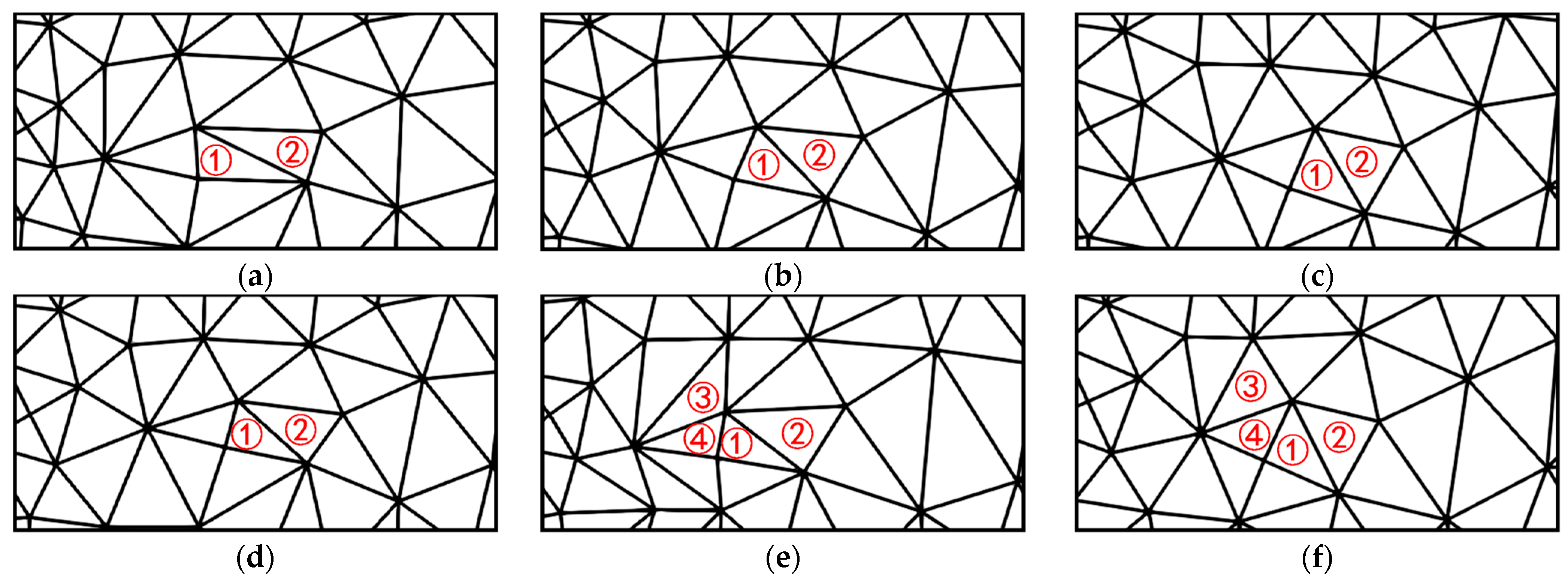
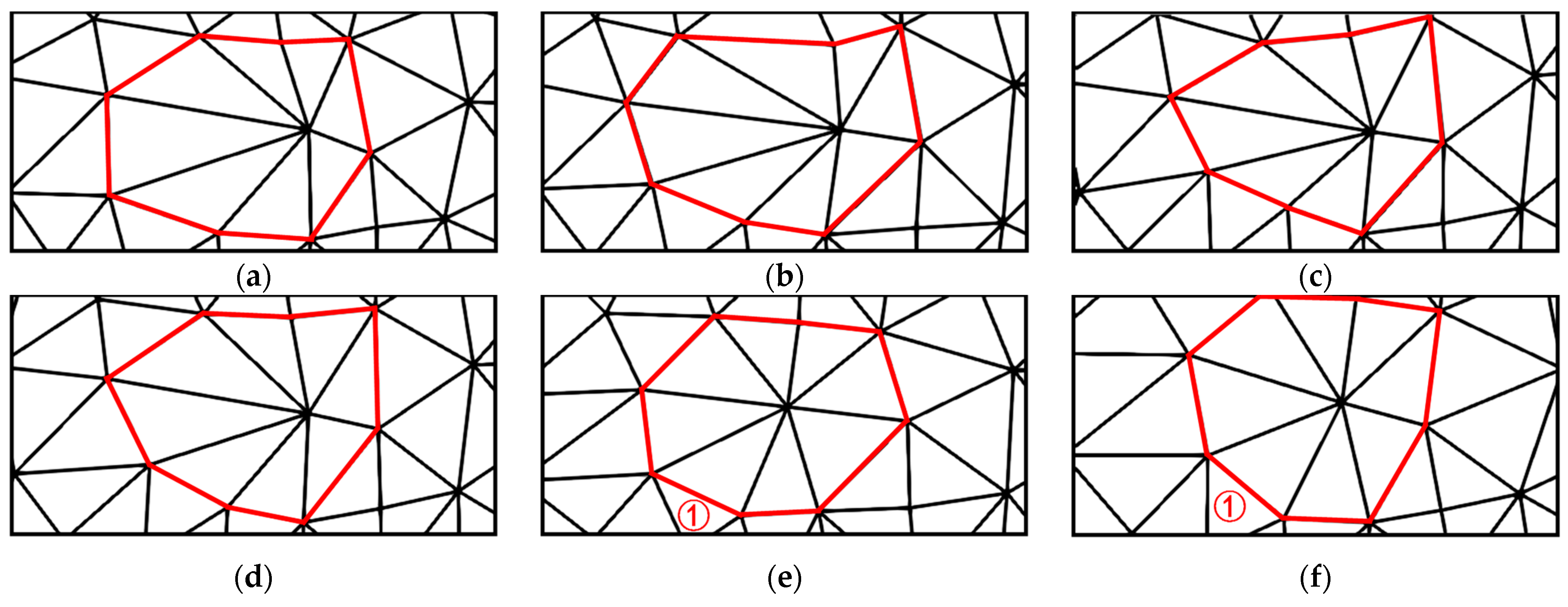
Moreover, due to the high quality of the meshes after Laplacian smoothing in Examples 1–4, the paper further analyzes the optimization effect of each method on the minimum angle of the element and the poor element shape. Figure 20a shows two distorted elements, element ① and element ②, in Example 1 after Laplacian smoothing, indicating that the Laplacian cannot handle poor elements well. From Figure 20b,e, it can be seen that the shapes of these two poor elements are still not well improved after being optimized using other methods. Compared with Figure 20e,f, the constrained DQN optimization will result in two poor elements: element ③ and element ④. However, the algorithm proposed in this paper can effectively improve the shape of elements ① and ② without generating poor elements.

Figure 20. Example 1—local comparison of each method after smoothing. (a) Laplacian; (b) angle-based; (c) ODT; (d) CVT; (e) unconstrained DQN; and (f) constrained DQN.

As shown in Figure 21a–e, after optimization, element ① still maintains its narrow and elongated shape. And, this algorithm can effectively improve the shape of element ①, as shown in Figure 21f.

Figure 21. Example 2—local comparison of each method after smoothing. (a) Laplacian; (b) angle-based; (c) ODT; (d) CVT; (e) unconstrained DQN; and (f) constrained DQN.

As shown in Figure 22, the six methods have similar optimization effects for Example 3. As shown in Figure 23a–d, Example 4 still has many poor elements after smoothing through Laplacian, angle-based, ODT, and CVT. The polygon formed by these poor elements is marked with red lines. Due to the influence of geometric shapes, the improvement effect of these four methods on low-quality elements is limited. Comparing Figure 23e,f, both unconstrained and constrained DQN can improve the shape of these poor elements, but the quality of element ① in Figure 23f is significantly higher than that in Figure 23e.

Figure 22. Example 3—local comparison of each method after smoothing. (a) Laplacian; (b) angle-based; (c) ODT; (d) CVT; (e) unconstrained DQN; and (f) constrained DQN.

Figure 23. Example 4—local comparison of each method after smoothing. (a) Laplacian; (b) angle-based; (c) ODT; (d) CVT; (e) unconstrained DQN; and (f) constrained DQN.

The optimization effect for low-quality elements also needs to consider the number of poor elements after optimization. First, there are no elements with a quality of less than 0.5 in the initial mesh. Second, elements with aspect ratio values of less than 0.8 are called low-quality elements. In summary, to investigate the optimization effect of the proposed method for low-quality elements, all elements of the four examples were taken as a whole, and the distribution of element quality between 0.5 and 0.8 was counted; the results are shown in Figure 24. It can be seen that the proposed method has the lowest number of poor elements after optimization, which also shows the advantage of the algorithm in improving the quality of poor elements in this paper.

Figure 24. Distribution of quality between 0.5 and 0.8.

4.4. Comparative Analysis of Experiments

In this paper, finite element analysis is carried out using two arithmetic examples to verify the superiority of the proposed method. Example 1 is an L-shaped plate with 788 elements and 435 nodes; Example 2 is a gravity dam with 3178 elements and 1665 nodes.

4.4.1. Example 1

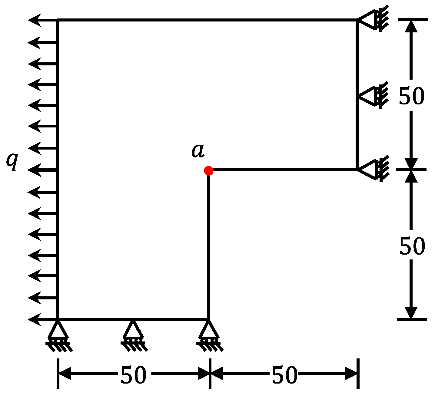
We selected the L-shaped flat plate [29] as Example 1. The area near the right angle inside is prone to stress concentration. Therefore, various methods were used to smooth Example 1, and the smoothed mesh was calculated with the finite element calculation method.

The geometric shape and load form of Example 1 are shown in Figure 25. The maximum length and width of the L-shaped flat plate are 100 mm, with a mass density of ρ = 7800 kg/m³, elastic modulus E = 206 Gpa, Poisson’s ratio μ = 0.3, and uniformly distributed load q = 1 N/mm².

Figure 25. L-shaped flat plate.

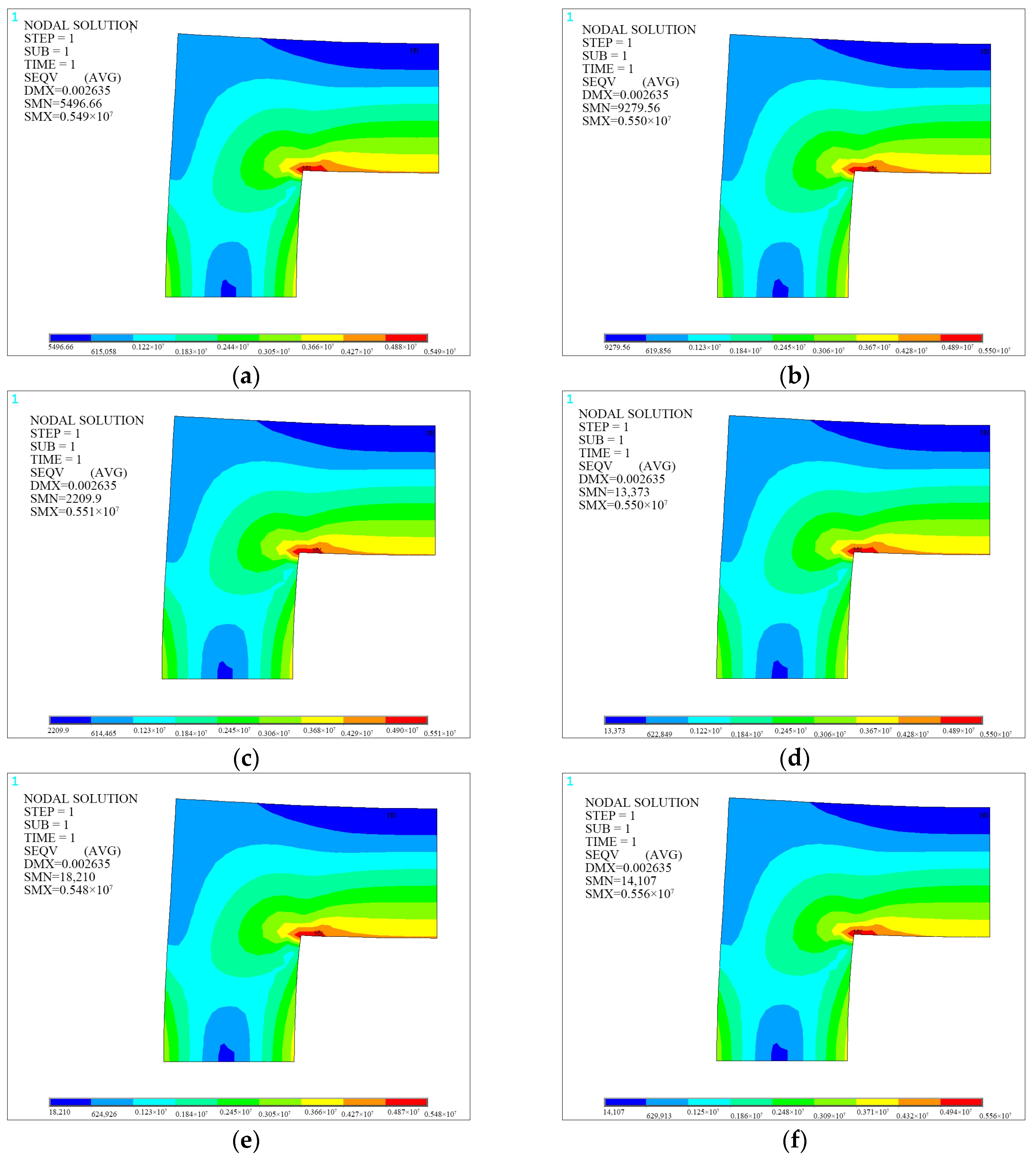
The initial, overall refined, and optimized mesh of the proposed method for Example 1 is shown in Figure 26. The comparison results of different methods are shown in Table 5. It can be seen that the proposed method is significantly better than the other methods for angle control. Since there is no analytical solution for the L-shaped plate, we used the finite element calculation results of the refined mesh, as shown in Figure 26b, as the reference solution for comparison. The stress nephograms for the initial and refined meshes of Example 1 are shown in Figure 27. The stress nephograms after optimization using the remaining optimization methods are shown in Figure 28.

Figure 26. Initial mesh, overall refined mesh, and optimized mesh. (a) Before smoothing; (b) refined mesh; and (c) after smoothing.

Table 5. Comparison table of the experimental results.

Mesh	Method	Time/(s)	Nodes	Min. θ	Max. θ	(a)	(b)	Min. q	Avg. q
2	Initial	/		26.93	108.78	45	86	0.7003	0.8635
	Laplacian	0.1024		28.62	102.80	3	2	0.7139	0.9417
	Angle-based	0.2045		28.82	100.26	2	1	0.7517	0.9475
	ODT	0.1377	788	28.62	104.52	3	7	0.7139	0.9401
	CVT	0.1249		28.62	99.80	3	0	0.7139	0.9478
	Unconstrained DQN	0.3175		30.06	103.39	0	3	0.7403	0.9262
	Constrained DQN	0.3261		33.03	98.44	0	0	0.7954	0.9357

Figure 27. Finite element calculation results of Example 1. (a) Initial mesh; (b) refined mesh.

Figure 28. Example 1: finite element calculation results after smoothing for each optimization method. (a) Laplacian; (b) angle-based; (c) ODT; (d) CVT; (e) unconstrained DQN; and (f) constrained DQN.

The maximum stress selected is the stress at point A in Figure 25. The results of the finite element calculations are shown in Table 6. It can be seen that the finite element calculation results of the optimized mesh of the proposed method are closer to the reference solution with minimum error. Compared with the initial mesh, the proposed method reduces the error by about 7% and further reduces the error by about 1% compared to other methods.

Table 6. Errors in maximum stress of different optimized meshes.

Method	Nodes	Elements	Stress (Mpa)	Error (%)
Initial			5.1531	12.5939
Laplacian			5.4915	6.8524
Angle-based			5.5006	6.6984
ODT	435	788	5.5068	6.5934
CVT			5.4987	6.7310
Unconstrained DQN			5.4453	7.6354
Constrained DQN			5.5564	5.7523
Refinement	804	1496	5.8955	/

4.4.2. Example 2

In this section, the gravity dam model in [30] is chosen for the calculation example. The model contains two parts: the dam and foundation; the specific geometry and load form are shown in Figure 29. The dam body’s height is 100 m, the top length is 5 m, the bottom length is 70 m, the capacity is 2400 N/m³, elasticity E = 21 GPa, and the Poisson’s ratio μ = 0.167. The calculated depth of the dam foundation is 200 m, the length is 370 m, the capacity is 2500 N/m³, elastic modulus E = 20 GPa, and the Poisson’s ratio μ = 0.17.

Figure 29. Gravity dam.

The initial mesh of the gravity dam and the optimized mesh are shown in Figure 30. The comparison results of different methods of optimization are shown in Table 7. According to Table 7, it can be seen that the proposed method is optimized for poor elements, and the minimum angle of the element is better controlled compared to other methods. Although ODT and CVTC have a shorter time, their optimization effects on complex models’ minimum and maximum angles are insignificant.

Figure 30. Example 2—comparison before and after smoothing. (a) Before smoothing; (b) after smoothing.

Table 7. Comparison table of the experimental results.

Mesh	Method	Time/(s)	Nodes	Min. θ	Max. θ	(a)	(b)	Min. q	Avg. q
2	Initial	/		8.32	153.96	1562	1095	0.2190	0.7312
	Laplacian	0.6207		26.52	111.37	12	24	0.6683	0.9507
	Angle-based	0.6969		26.52	111.32	11	21	0.6679	0.9411
	ODT	0.7397	1665	14.30	148.60	27	40	0.3159	0.9336
	CVT	0.8148		16.93	135.92	25	32	0.6355	0.9437
	Unconstrained DQN	1.2549		27.09	127.17	33	30	0.5264	0.9188
	Constrained DQN	1.3166		31.01	108.64	0	2	0.6814	0.9372

The finite element calculation results of the initial mesh are shown in Figure 31. The finite element calculation results of the mesh after optimization with different methods are shown in Figure 32.

Figure 31. Finite element calculation results of the initial mesh. (a) Global; (b) local.

Figure 32. Example 2: finite element calculation results after smoothing for each optimization method. (a) Laplacian; (b) angle-based; (c) ODT; (d) CVT; (e) unconstrained DQN; and (f) constrained DQN.

Since the stress concentration problem occurs at point A in Figure 29 in actual engineering, the stress values in the x- and y-direction at point A are extracted, and the calculation results of the proposed method are compared with other methods; the data statistics are shown in Table 8. According to Table 8, it is easy to find that the computational results of the optimized mesh of the proposed method for finite element analysis are closer to the results in [30] with minimum errors. Although the average error of the results smoothed using Laplacian is small, the error in the x-direction is relatively large.

Table 8. Comparison table of finite element calculation results.

Method	Nodes	Element	Stress (x)	Error (x)	Stress (x)	Error (y)	Mean Error
Initial	1665	3178	9.6259	30.25	10.2441	30.03	30.14
Laplacian			9.9706	27.75	10.9232	22.34	25.04
Angle-based			9.8940	28.30	10.9515	25.19	26.75
ODT			9.7165	29.59	10.6509	27.25	28.42
CVT			9.7404	29.42	10.8809	25.68	27.55
Unconstrained DQN			10.0845	26.92	11.2019	23.48	25.20
Constrained DQN			10.6940	22.51	11.8218	19.25	20.88
Reference [30]	8263	10,270	13.8000	/	14.6400	/	/

Note: The unit of stress is Mpa.

This section verifies the lifting effect of the proposed method for finite element calculations using two examples. The effect of improving the accuracy of finite element calculation is achieved by optimizing the minimum angle and improving the minimum element quality.

5. Conclusions

This paper proposes a planar Delaunay mesh smoothing method based on angle and a deep Q-network. Firstly, the central node based on the vertex angle of the bisected polygon is updated, and the convex hull algorithm is used to construct the inner polygon for the updated scattered points. In addition, to address the problem of low generalization of the unconstrained DQN model, an inner polygon is proposed to be iteratively updated with repeated training of reinforcement learning, and the updated inner polygon is used as the basis for the reward function setting during neural network training. The effectiveness of this method was demonstrated through simple examples and meshes with size gradient features. Moreover, a large number of untrained examples were used to verify the high generalization of the DQN model trained using this method. Additionally, the comparison experiments of this paper’s method with Laplacian, angle-based, ODT, CVT, and unconstrained DQN on four examples show that this paper’s method can better control the minimum angle, improve the minimum quality, and reduce the number of poor elements. Finally, two numerical examples were used for finite element analysis to verify the improvement effect of the proposed method on the finite element calculation results.

This study explores the impact of the constructed inner polygon on a deep Q-based network smoothing method and improves the performance of the DQN model. Although some achievements have been made, many problems need to be solved. One problem is that the proposed method only focuses on triangular elements as the research object. However, the element types also include quadrilateral elements, tetrahedron elements, Hexahedron elements, etc. In future work, we plan to expand our research on element types, construct inner polygon or even inner polyhedra, and use reinforcement learning methods to study the mesh. Finally, we will also research the latest deep network structures to shorten training time.

References

- Kim, J.; Sastry, S.P.; Shontz, S.M. A numerical investigation on the interplay amongst geometry, meshes, and linear algebra in the finite element solution of elliptic PDEs. Eng. Comput. 2012, 28, 431–450. [Google Scholar] [CrossRef]
- Cheng, S.W.; Dey, T.K.; Shewchuk, J. 1.2 Delaunay triangulations and Delaunay refinement. In Delaunay Mesh Generation, 1st ed.; CRC Press: Boca Raton, FL, USA, 2013; pp. 8–10. [Google Scholar] [CrossRef]
- Strang, G.; Fix, G.J.; Griffin, D.S. An Analysis of the Finite-Element Method. ASME J. Appl. Mech. 1974, 41, 62. [Google Scholar] [CrossRef]
- Babuška, I.; Aziz, A.K. On the angle condition in the finite element method. SIAM J. Numer. Anal. 1976, 13, 214–226. [Google Scholar] [CrossRef]
- Shewchuk, J. What is a good linear finite element? interpolation, conditioning, anisotropy, and quality measures (preprint). Univ. Calif. Berkeley 2002, 73, 137. [Google Scholar]
- Durand, R.; Pantoja-Rosero, B.G.; Oliveira, V. A general mesh smoothing method for finite elements. Finite Elem. Anal. Des. 2019, 158, 17–30. [Google Scholar] [CrossRef]
- Huang, X.; Xu, D. Aspect-ratio based triangular mesh smoothing. In ACM SIGGRAPH 2017 Posters; Association for Computing Machinery: New York, NY, USA, 2017; pp. 1–2. [Google Scholar] [CrossRef]
- Field, D.A. Laplacian smoothing and delaunay triangulations. Commun. Appl. Numer. Methods 1988, 4, 709–712. [Google Scholar] [CrossRef]
- Blacker, T.D.; Stephenson, M.B. Paving: A new approach to automated quadrilateral mesh generation. Int. J. Numer. Methods Eng. 1991, 32, 811–847. [Google Scholar] [CrossRef]
- Zhu, J.Z.; Zienkiewicz, O.C.; Hinton, E.; Wu, J. A new approach to the development of automatic quadrilateral mesh generation. Int. J. Numer. Methods Eng. 1991, 32, 849–866. [Google Scholar] [CrossRef]
- Freitag, L.A.; Ollivier-Gooch, C. A Comparison of Tetrahedral Mesh Improvement Techniques; Argonne National Lab. (ANL): Argonne, IL, USA, 1996. [Google Scholar] [CrossRef]
- Canann, S.A.; Tristano, J.R.; Staten, M.L. An approach to combined Laplacian and optimization-based smoothing for triangular, quadrilateral, and quad-dominant meshes. IMR 1998, 1, 479–494. [Google Scholar]
- Freitag, L.A. On Combining Laplacian and Optimization-Based Mesh Smoothing Techniques; Argonne National Lab. (ANL): Argonne, IL, USA, 1997. [Google Scholar]
- Zhou, T.; Shimada, K. An angle-based approach to two-dimensional mesh smoothing. IMR 2000, 2000, 373–384. [Google Scholar]
- Xu, H.T.; Newman, T.S. An angle-based optimization approach for 2D finite element mesh smoothing. Finite Elem. Anal. Des. 2006, 42, 1150–1164. [Google Scholar] [CrossRef]
- Gong, X.F.; Zhang, S.D. One mesh smoothing algorithm combining Laplacian and local optimization-based mesh smoothing techniques. Trans. Beijing Inst. Technol. 2010, 30, 616–621. (In Chinese) [Google Scholar]
- Lee, E.; Shin, M.; Kim, J. Improved simultaneous mesh untangling and quality improvement methods of 2D triangular meshes. Int. J. Comput. Methods 2019, 16, 1850119. [Google Scholar] [CrossRef]
- Kim, J.; Panitanarak, T.; Shontz, S.M. A multiobjective mesh optimization framework for mesh quality improvement and mesh untangling. Int. J. Numer. Methods Eng. 2013, 94, 20–42. [Google Scholar] [CrossRef]
- Mittal, K.; Fischer, P. Mesh smoothing for the spectral element method. J. Sci. Comput. 2019, 78, 1152–1173. [Google Scholar] [CrossRef]
- Kim, J. An efficient approach for solving mesh optimization problems using newton’s method. Math. Probl. Eng. 2014, 2014, 273732. [Google Scholar] [CrossRef]
- Roda-Casanova, V.; Sanchez-Marin, F. A simple procedure for generating locally refined 2D quadrilateral finite element meshes of gears. Mech. Mach. Theory 2021, 157, 104185. [Google Scholar] [CrossRef]
- Kim, J.; Shin, M.; Kang, W. A derivative-free mesh optimization algorithm for mesh quality improvement and untangling. Math. Probl. Eng. 2015, 2015, 264741. [Google Scholar] [CrossRef]
- Alliez, P.; Cohen-Steiner, D.; Yvinec, M.; Desbrun, M. Variational tetrahedral meshing. In ACM SIGGRAPH 2005 Papers; Association for Computing Machinery: New York, NY, USA, 2005; pp. 617–625. [Google Scholar] [CrossRef]
- Du, Q.; Gunzburger, M. Grid generation and optimization based on centroidal Voronoi tessellations. Appl. Math. Comput. 2002, 133, 591–607. [Google Scholar] [CrossRef]
- Guo, Y.F.; Wang, C.R.; Ma, Z.; Huang, X.H.; Sun, K.W.; Zhao, R.L. A new mesh smoothing method based on a neural network. Comput. Mech. 2022, 69, 425–438. [Google Scholar] [CrossRef]
- Kim, J.; Choi, J.; Kang, W. A data-driven approach for simultaneous mesh untangling and smoothing using Pointer networks. IEEE Access 2020, 8, 70329–70342. [Google Scholar] [CrossRef]
- Zhang, H.J.; Liu, X.; Li, H.J. Deep Q network-based optimization algorithm for planar Delaunay mesh. J. Comput.-Aided Des. Comput. Graph. 2022, 34, 1943–1950. [Google Scholar] [CrossRef]
- Virtanen, P.; Gommers, R.; Oliphant, T.E.; Haberland, M.; Reddy, T.; Cournapeau, D.; Burovski, E.; Peterson, P.; Weckesser, W.; Bright, J.; et al. SciPy 1.0: Fundamental algorithms for scientific computing in Python. Nat. Methods 2020, 17, 261–272. [Google Scholar] [CrossRef] [PubMed]
- Zienkiewicz, O.C.; Zhu, J.Z.; Gong, N.G. Effective and practical h–p-version adaptive analysis procedures for the finite element method. Int. J. Numer. Methods Eng. 1989, 28, 879–891. [Google Scholar] [CrossRef]
- Yang, Q.; Wu, H.; Zhou, W.Y. Stress evaluation in finite element analysis of dams. Eng. Mech. 2006, 23, 69–73. (In Chinese) [Google Scholar]
Disclaimer/Publisher’s Note: The statements, opinions and data contained in all publications are solely those of the individual author(s) and contributor(s) and not of MDPI and/or the editor(s). MDPI and/or the editor(s) disclaim responsibility for any injury to people or property resulting from any ideas, methods, instructions or products referred to in the content. |
© 2023 by the authors. Licensee MDPI, Basel, Switzerland. This article is an open access article distributed under the terms and conditions of the Creative Commons Attribution (CC BY) license (https://creativecommons.org/licenses/by/4.0/).