


A Hybrid Prediction Model for Local Resistance Coefficient of Water Transmission Tunnel Maintenance Ventilation Based on Machine Learning

Abstract
:1. Introduction
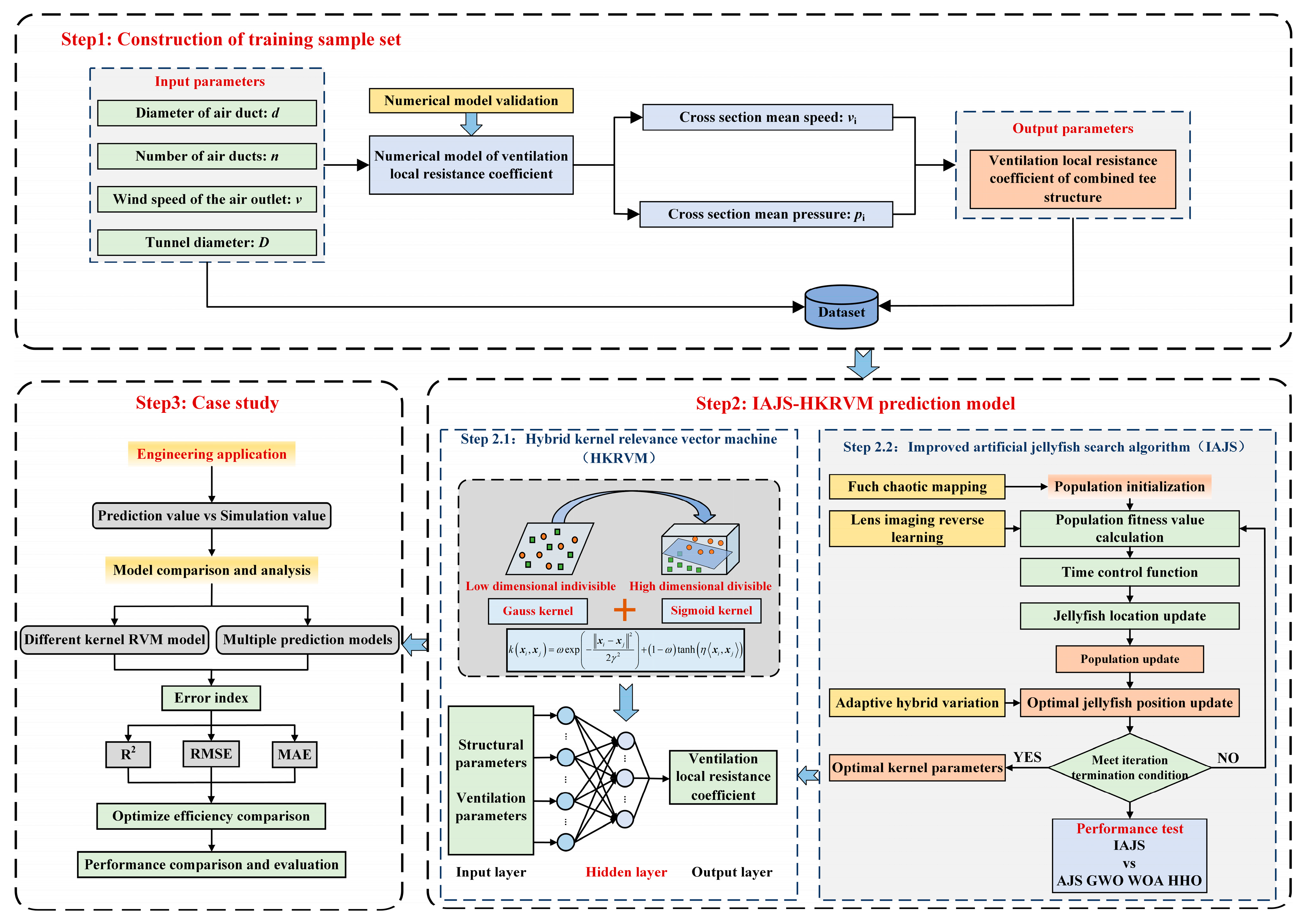
2. Research Framework
3. Methodology
3.1. IAJS-HKRVM Model
3.1.1. Hybrid Kernel Relevance Vector Machine
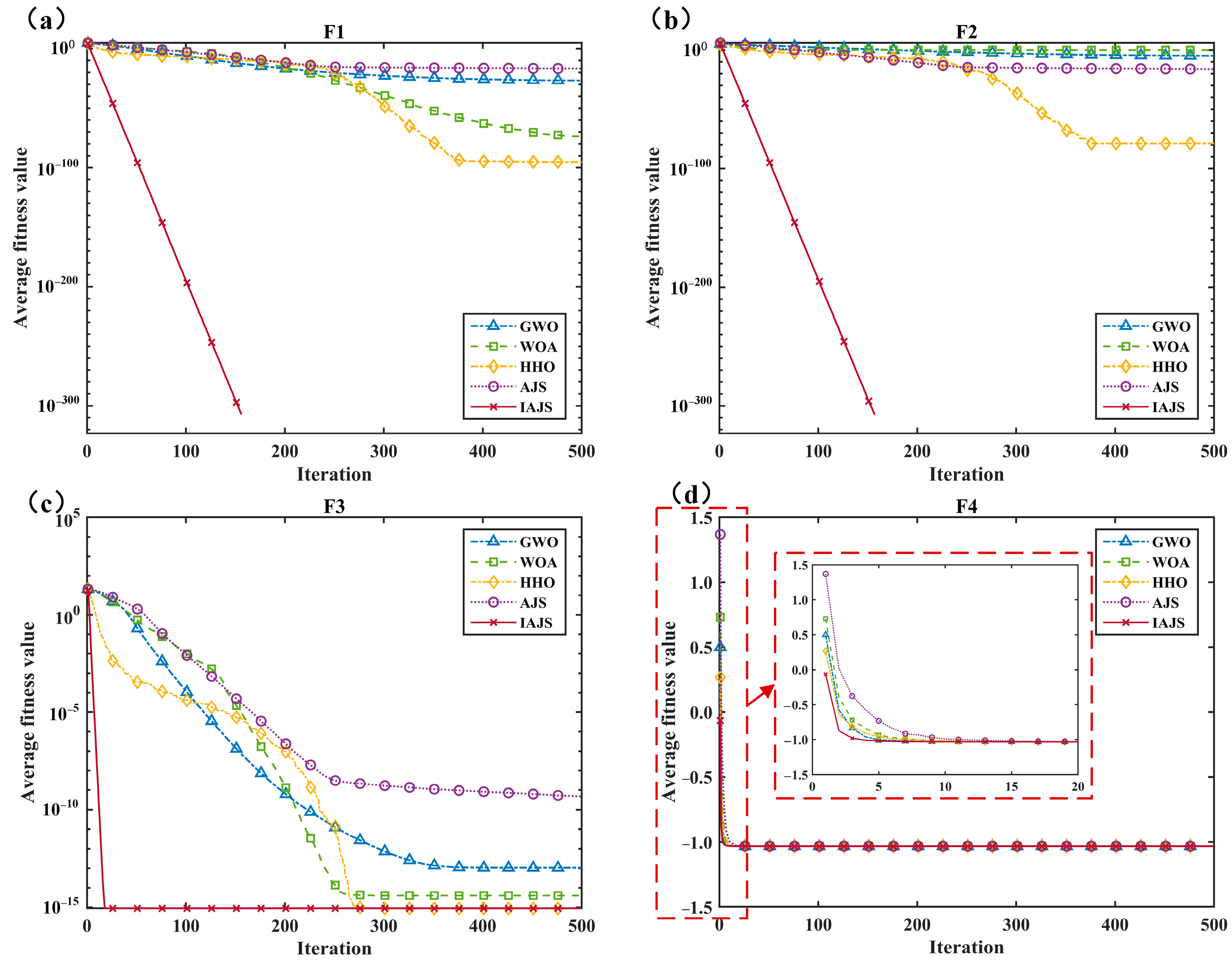
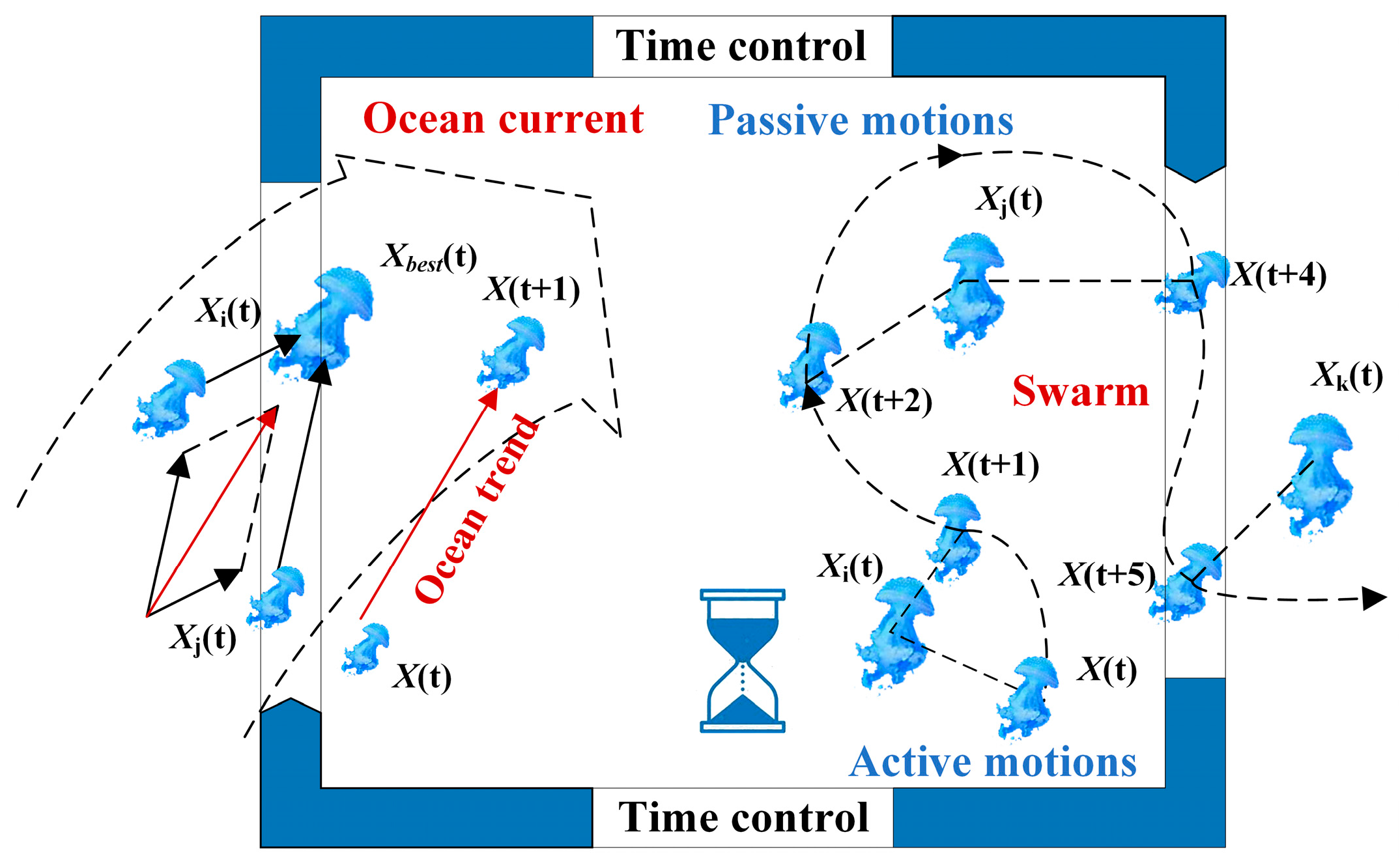
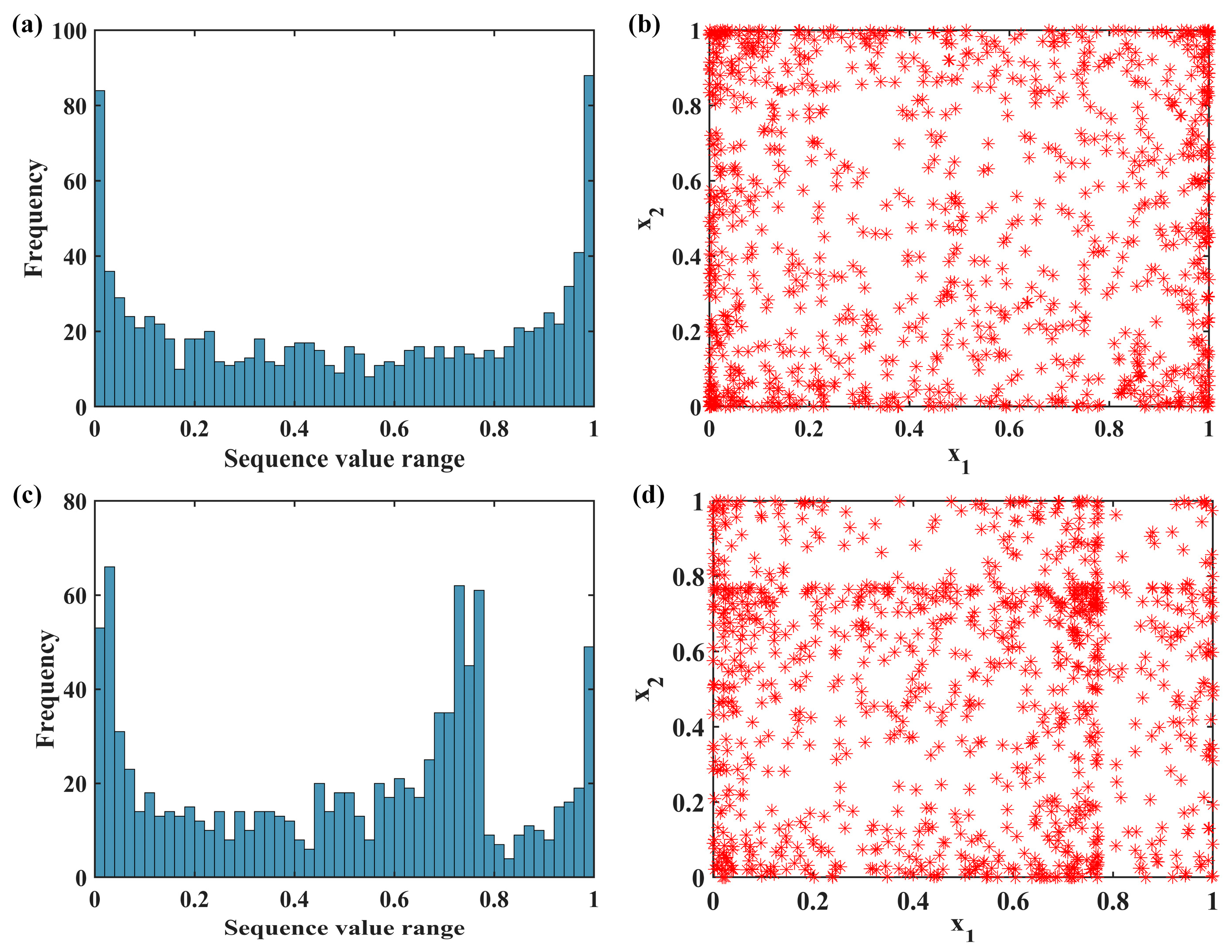
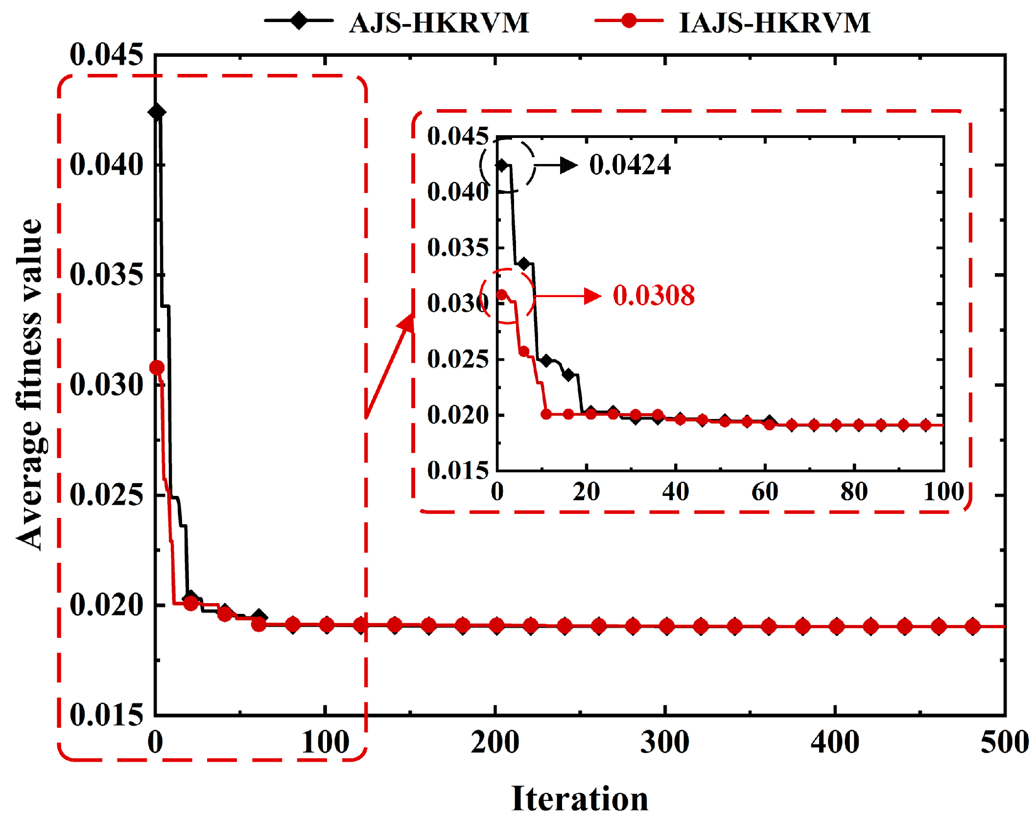
3.1.2. Improved Artificial Jellyfish Search Algorithm
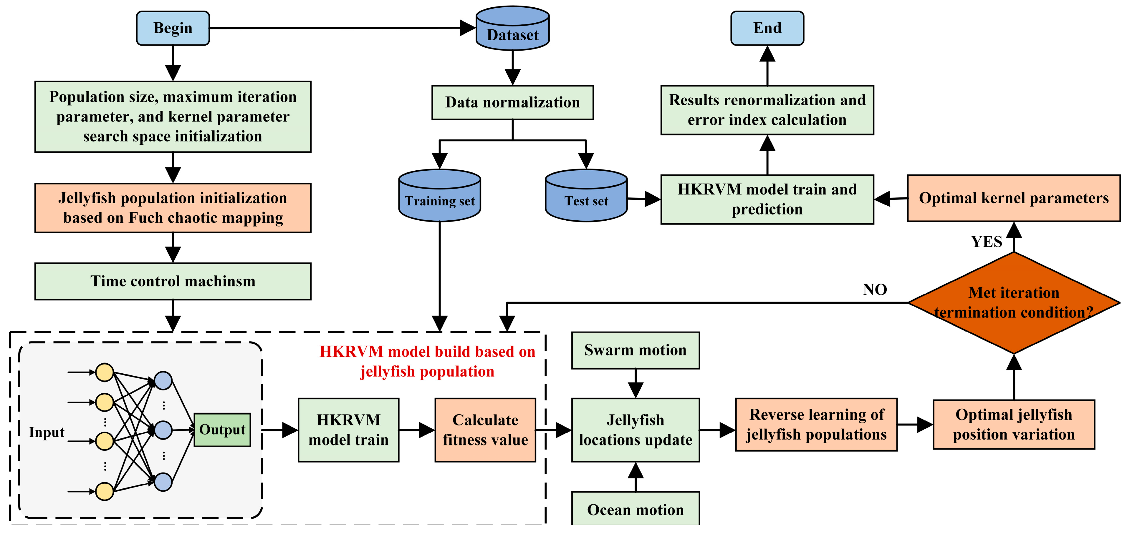
3.2. Establishment Process of the Hybrid Prediction Model for Local Resistance Coefficient of Water Transmission Tunnel Maintenance Ventilation Based on Machine Learning
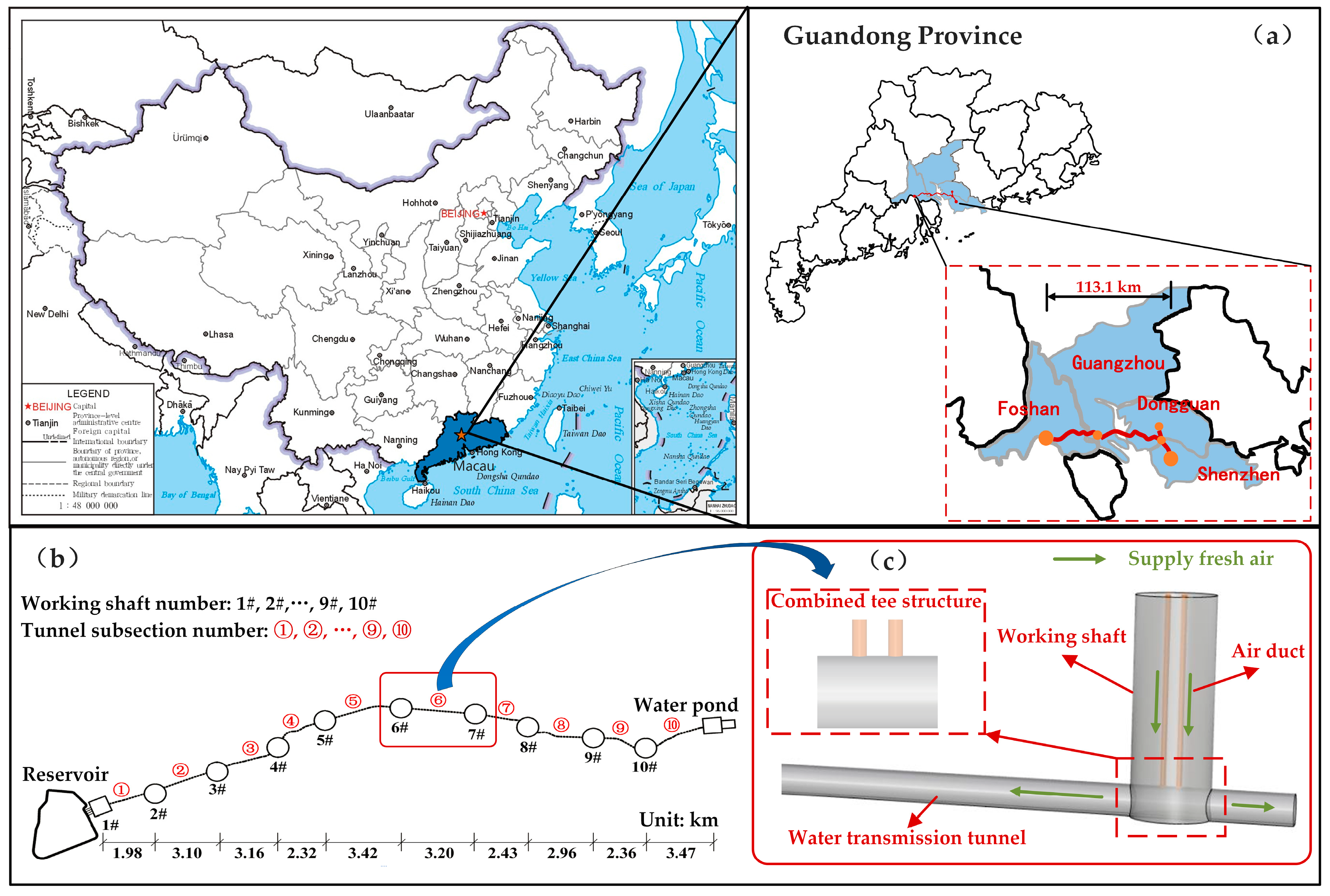
4. Case Study
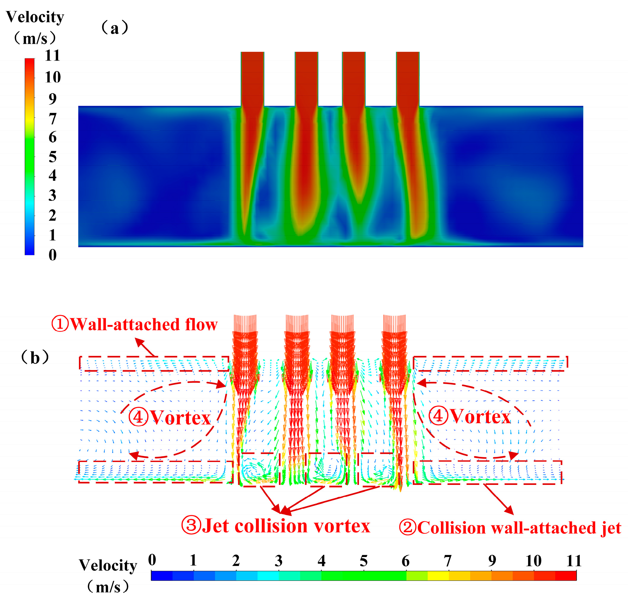
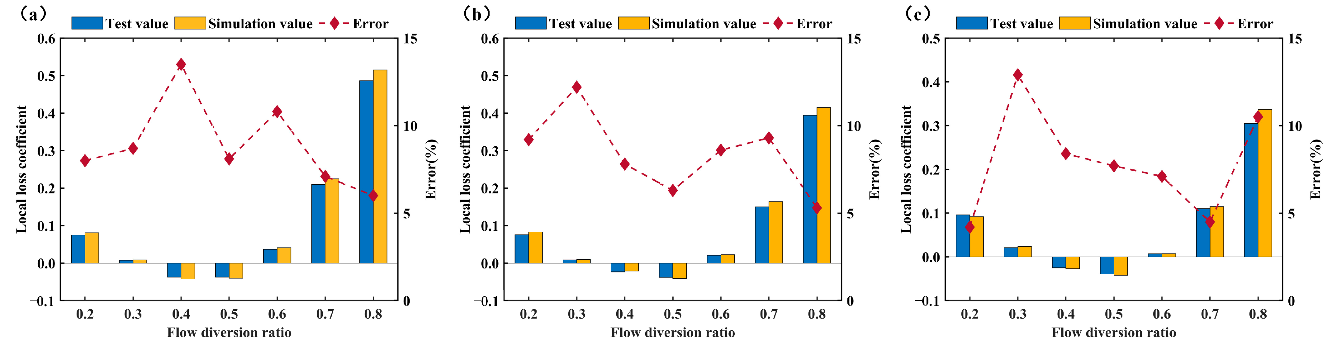
4.1. Analysis of Ventilation Local Resistance Characteristics
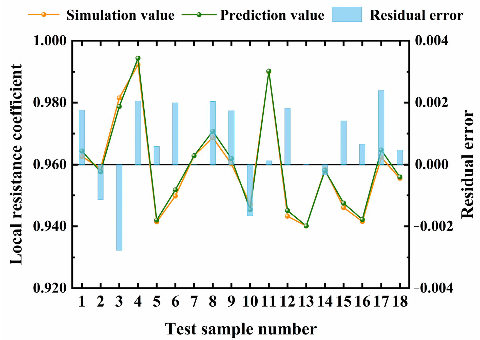
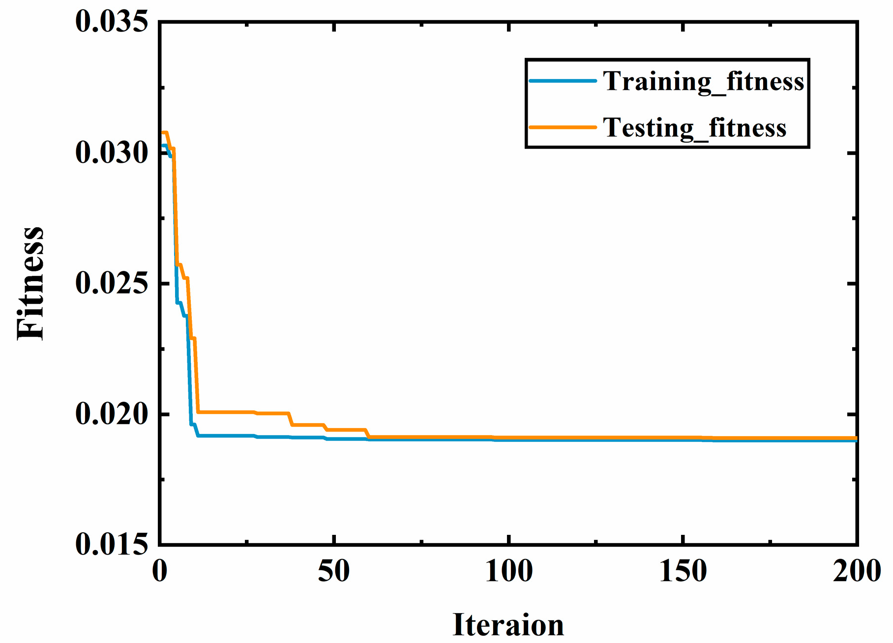
4.2. Analysis of Prediction Results for Ventilation Local Resistance Coefficient
5. Discussion
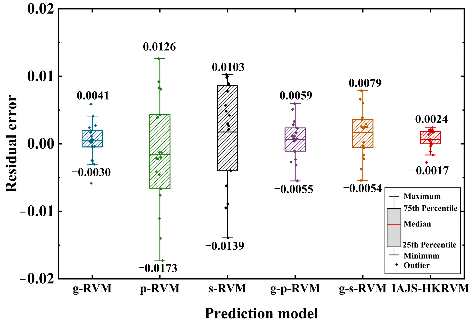
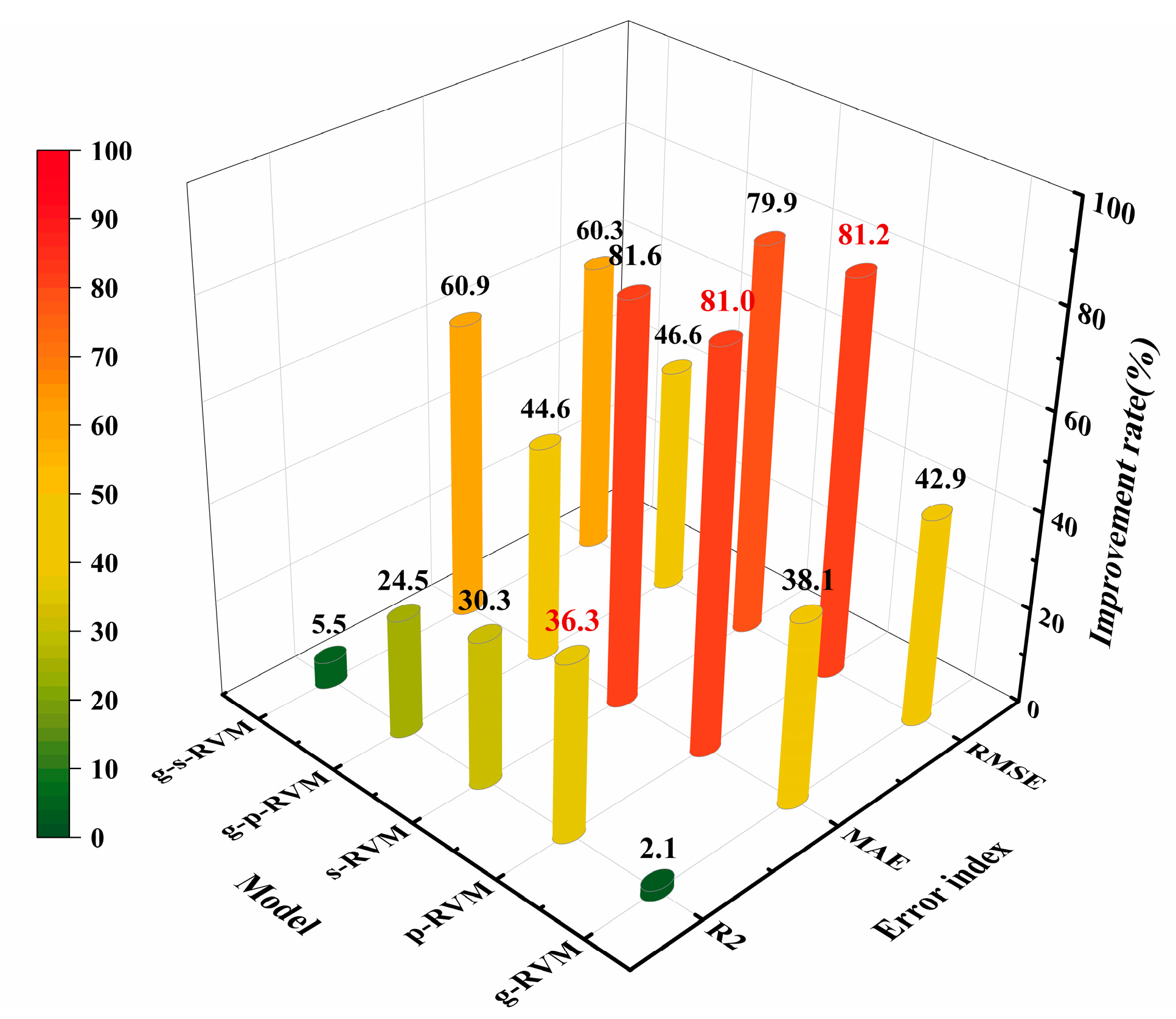
5.1. Comparison with Conventional RVM Models
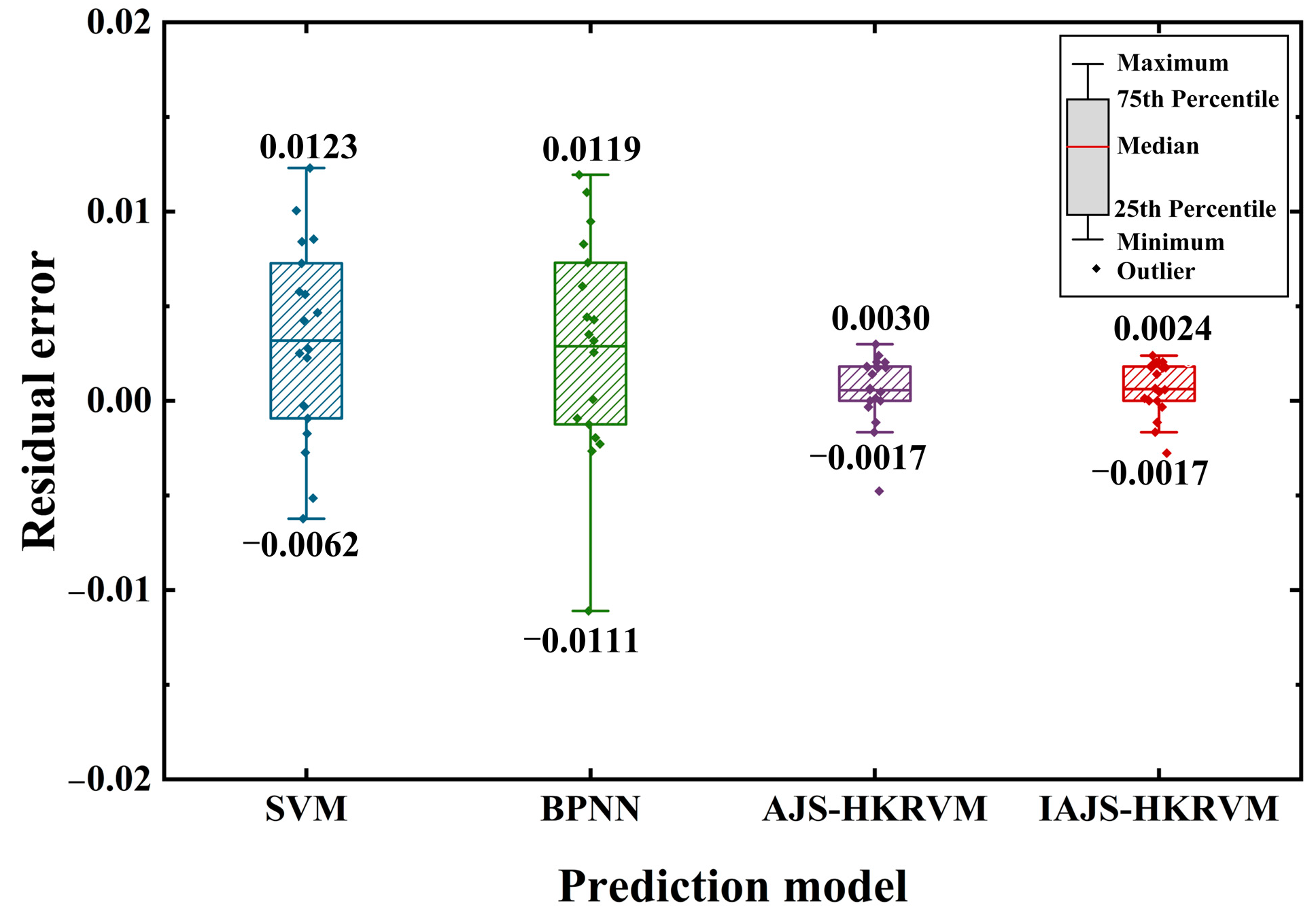
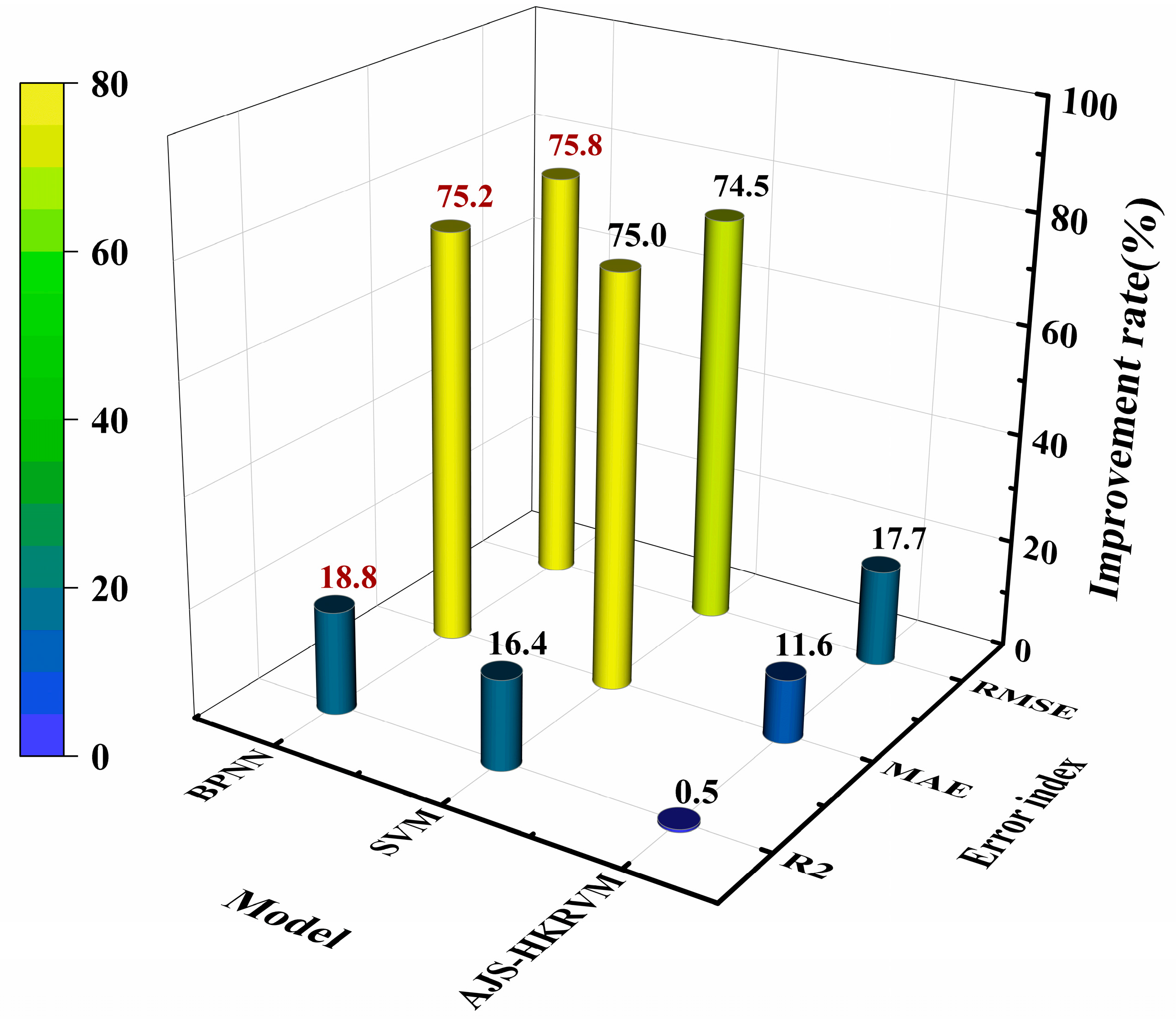
5.2. Comparison with Other Prediction Models
6. Conclusions
Author Contributions
Funding
Institutional Review Board Statement
Informed Consent Statement
Data Availability Statement
Acknowledgments
Conflicts of Interest
Abbreviations
| HKRVM | Hybrid kernel relevance vector machine |
| IAJS | Improved artificial jellyfish search algorithm |
| RVM | Relevance vector machine |
| AJS | Artificial jellyfish search algorithm |
| SVM | Support vector machine |
| BPNN | Backpropagating neural network |
| R2 | Relative coefficient square |
| MAE | Mean absolute error |
| RMSE | Root mean square error |
| GWO | Grey wolf optimization algorithm |
| WOA | Whale optimization algorithm |
| HHO | Harris hawks optimization algorithm |
References
- Zhang, C.; Nong, X.Z.; Shao, D.G.; Zhong, H.; Shang, Y.M.; Liang, J.K. Multivariate water environmental risk analysis in long-distance water supply project: A case study in China. Ecol. Indic. 2021, 125, 70–82. [Google Scholar] [CrossRef]
- Liu, D.M.; Hong, J.; Wang, R.; Cui, F.Y. Current solution to Limnoperna fortunei problem in water and pipelines. In Proceedings of the 2011 2nd International Conference on Artificial Intelligence, Management Science and Electronic Commerce (AIMSEC), Dengfeng, China, 8–10 August 2011. [Google Scholar]
- Zhang, C.D.; Xu, M.Z.; Wang, Z.Y.; Liu, W.; Yu, D.D. Experimental study on the effect of turbulence in pipelines on the mortality of Limnoperna fortunei veligers. Ecol. Eng. 2017, 109, 101–118. [Google Scholar] [CrossRef]
- Liu, C.X.; Wang, X.L.; Tong, D.W.; Liu, Z.; Yang, C.; Chen, S.; Wang, R.N.; Ding, C.Y. Impact of various multishaft combined ventilation modes on the removal of harmful gases released from mussel decay in a long-distance water conveyance tunnel. Tunn. Undergr. Space Technol. 2022, 128, 104633. [Google Scholar] [CrossRef]
- Crapper, M.; Motta, D.; Sinclair, C.; Cole, D.; Monteleone, M.; Cosheril, A.; Tree, J.; Parkin, A. The hydraulic characteristics of Roman lead water pipes: An experimental investigation. Int. J. Hist. Eng. Technol. 2022, 91, 119–134. [Google Scholar] [CrossRef]
- Baselt, I.; Malcherek, A. Determining the Flow Resistance of Racks and the Resulting Flow Dynamics in the Channel by Using the Saint-Venant Equations. Water 2022, 14, 2469. [Google Scholar] [CrossRef]
- Wang, X.; Tan, W.; Ma, J.; Wang, L. Study on local structural resistance of ventilation system in highway tunnels. Mod. Tunn. Technol. 2019, 56, 104–113. (In Chinese) [Google Scholar]
- Wang, X.; Wang, M.N.; Qin, P.C.; Yan, T.; Chen, J.; Deng, T.; Yu, L.; Yan, G.F. An experimental study on the influence of local loss on ventilation characteristic of dividing flow in urban traffic link tunnel. Build. Sci. 2020, 174, 106793. [Google Scholar] [CrossRef]
- Liang, C.J.; Nan, S.; Shao, X.L.; Li, X.T. Calculation method for air resistance coefficient of vehicles in tunnel with different traffic conditions. J. Build. Eng. 2021, 44, 102971. [Google Scholar] [CrossRef]
- Wang, N.; Li, Y.C.; Zhang, H.; Zhang, J.; Li, B.L. Study on flow distribution and local resistance characteristics of louvered windshield. J. Saf. Sci. Technol. 2022, 18, 118–123. (In Chinese) [Google Scholar]
- Li, S.; Liu, X.F.; Wang, J.X.; Zheng, Y.L.; Deng, S.M. Experimental reduced-scale study on the resistance characteristics of the ventilation system of a utility tunnel under different pipeline layouts. Tunn. Undergr. Space Technol. 2019, 90, 131–143. [Google Scholar] [CrossRef]
- Wang, H.D.; Li, X.H.; Tang, Y.; Chen, X.W.; Shen, H.H.; Cao, X.C.; Gao, H.M. Simulation and experimental study on the elbow pressure loss of large air duct with different internal guide vanes. Build Serv. Eng. Res. Technol. 2022, 43, 725–739. [Google Scholar] [CrossRef]
- Li, Y.F.; Chang, J.T.; Kong, C.; Bao, W. Recent progress of machine learning in flow modeling and active flow control. Chin. J. Aeronaut. 2022, 35, 14–44. [Google Scholar] [CrossRef]
- Hammond, J.; Pepper, N.; Montomoli, F.; Michelassi, V. Machine Learning Methods in CFD for Turbomachinery: A review. Int. J. Turbomach. Propuls. Power 2022, 7, 16. [Google Scholar] [CrossRef]
- Mostafa, K.; Zisis, I.; Moustafa, M.A. Machine learning Techniques in Structural Wind Engineering: A state-of-the-art review. Appl. Sci. 2022, 12, 5232. [Google Scholar] [CrossRef]
- Li, Y.; Huang, X.; Li, Y.G.; Chen, F.B.; Li, Q.S. Machine learning based algorithms for wind pressure prediction of high-rise buildings. Adv. Struct. Eng. 2022, 25, 2222–2233. [Google Scholar] [CrossRef]
- Zhu, Q.M.; Zhao, Z.; Yan, J.H. Physics-informed machine learning for surrogate modeling of wind pressure and optimization of pressure sensor placement. Comput. Mech. 2022, 71, 481–491. [Google Scholar] [CrossRef]
- Hu, Z.L.; Karami, H.; Rezaei, A.; DadrasAjirlou, Y.; Piran, M.J.; Band, S.S.; Chau, K.W.; Mosavi, A. Using soft computing and machine learning algorithms to predict the discharge coefficient of curved labyrinth overflows. Eng. Appl. Comp. Fluid Mech. 2021, 15, 1002–1015. [Google Scholar] [CrossRef]
- Wakes, S.J.; Bauer, B.O.; Mayo, M. A preliminary assessment of machine learning algorithms for predicting CFD-simulated wind flow patterns over idealized foredunes. J. R. Soc. N. Z. 2021, 51, 290–306. [Google Scholar] [CrossRef]
- Rush, S.; Rahman, M.; Arifuzzaman, M.; Ali, S.A.; Shalabi, F.; Aktaruzzaman, M. Predicting pressure losses in the water-assisted flow of unconventional crude with machine learning. Pet. Sci. Technol. 2021, 39, 926–943. [Google Scholar] [CrossRef]
- Liu, Y.Q. Study on the air quantity of mine ventilation network based on BP neural network prediction model of friction resistance coefficient in roadway. Min. Saf. Environ. Prot. 2021, 48, 101–106. (In Chinese) [Google Scholar]
- Gao, K.; Deng, L.J.; Liu, J.; Wen, L.X.; Wong, D.; Liu, Z.Y. Study on mine ventilation resistance coefficient inversion based on genetic algorithm. Arch. Min. Sci. 2018, 63, 813–826. [Google Scholar]
- Tipping, M.E. Sparse Bayesian learning and the relevance vector machine. J. Mach. Learn. Res. 2001, 1, 211–244. [Google Scholar]
- Guo, R.X.; Wang, Y.G. Remaining useful life prognostics for the rolling bearing based on a hybrid data-driven method. Proc. Inst. Mech. Eng. Part I–J Syst. Control Eng. 2021, 235, 517–531. [Google Scholar] [CrossRef]
- Pan, Q.J.; Leung, Y.F.; Hsu, S.C. Stochastic seismic slope stability assessment using polynomial chaos expansions combined with relevance vector machine. Geosci. Front. 2021, 12, 405–414. [Google Scholar] [CrossRef]
- Ding, J.; Wang, M.L.; Ping, Z.W.; Fu, D.F.; Vassiliadis, V.S. An integrated method based on relevance vector machine for short-term load forecasting. Eur. J. Oper. Res. 2020, 287, 497–510. [Google Scholar] [CrossRef]
- Huang, J.; Yang, X.; Shardt, Y.A.W.; Yan, X.F. Fault Classification in Dynamic Process Using Multiclass Relevance Vector Machine and Slow Feature Analysis. IEEE Access 2020, 8, 9115–9123. [Google Scholar] [CrossRef]
- Pham, Q.B.; Sammen, S.S.; Abba, S.I.; Mohammadi, B.; Shahid, S.; Abdulkadir, R.A. A new hybrid model based on relevance vector machine with flower pollination algorithm for phycocyanin pigment concentration estimation. Environ. Sci. Pollut. Res. 2021, 28, 32564–32579. [Google Scholar] [CrossRef]
- Qiu, J.S.; Fan, Y.C.; Wang, S.L.; Yang, X.; Qiao, J.L.; Liu, D.L. Research on the remaining useful life prediction method of lithium-ion batteries based on aging feature extraction and multi-kernel relevance vector machine optimization model. Int. J. Energy Res. 2022, 46, 13931–13946. [Google Scholar] [CrossRef]
- Tao, H.; Al-Bedyry, N.K.; Khedher, K.M.; Shahid, S.; Yaseen, Z.M. River water level prediction in coastal catchment using hybridized relevance vector machine model with improved grasshopper optimization. J. Hydrol. 2021, 598, 126477. [Google Scholar] [CrossRef]
- Song, W.S.; Guan, T.; Ren, B.Y.; Yu, J.; Wang, J.J.; Wu, B.P. Real-Time Construction Simulation Coupling a Concrete Temperature Field Interval Prediction Model with Optimized Hybrid-Kernel RVM for Arch Dams. Energies 2020, 13, 4487. [Google Scholar] [CrossRef]
- Zhao, Y.; Li, Z.Q. Import and Export Trade Prediction Algorithm of Belt and Road Countries Based on Hybrid RVM Model. Math. Probl. Eng. 2022, 2022, 6467326. [Google Scholar] [CrossRef]
- Wang, S.; Zhang, X.C.; Chen, W.X.; Han, W.; Zhou, S.B.; Pecht, M. State of health prediction based on multi-kernel relevance vector machine and whale optimization algorithm for lithium-ion battery. Trans. Inst. Meas. Control, 2021; ahead of print. [Google Scholar] [CrossRef]
- Bui, D.T.; Hoang, N.D.; Nguyen, H.; Tran, X.L. Spatial prediction of shallow landslide using Bat algorithm optimized machine learning approach: A case study in Lang Son Province, Vietnam. Adv. Eng. Inform. 2019, 42, 100978. [Google Scholar]
- Chou, J.S.; Truong, D.N. A novel metaheuristic optimizer inspired by behavior of jellyfish in ocean. Appl. Math. Comput. 2021, 389, 125535. [Google Scholar] [CrossRef]
- Shaheen, A.M.; El-Sehiemy, R.A.; Alharthi, M.M.; Ghoneim, S.S.M.; Ginidi, A.R. Multi-objective jellyfish search optimizer for efficient power system operation based on multi-dimensional OPF framework. Energy 2021, 237, 121478. [Google Scholar] [CrossRef]
- Farhat, M.; Kamel, S.; Atallah, A.M.; Khan, B. Optimal Power Flow Solution Based on Jellyfish Search Optimization Considering Uncertainty of Renewable Energy Sources. IEEE Access 2021, 9, 100911–100933. [Google Scholar] [CrossRef]
- Abdel-Basset, M.; Mohamed, R.; Abouhawwash, M.; Chakrabortty, R.K.; Ryan, M.J.; Nam, Y. An improved jellyfish algorithm for multilevel thresholding of magnetic resonance brain image segmentations. CMC-Comput. Mat. Contin. 2021, 68, 2961–2977. [Google Scholar] [CrossRef]
- Chou, J.S.; Liu, C.Y.; Prayogo, H.; Khasani, R.R.; Gho, D.; Lalitan, G.G. Predicting nominal shear capacity of reinforced concrete wall in building by metaheuristics-optimized machine learning. J. Build. Eng. 2022, 61, 105046. [Google Scholar] [CrossRef]
- Chou, J.S.; Karundeng, M.A.; Truong, D.N.; Cheng, M.Y. Identifying deflections of reinforced concrete beams under seismic loads by bio-inspired optimization of deep residual learning. Struct. Control Health Monit. 2022, 29, e2918. [Google Scholar] [CrossRef]
- Fu, W.Y.; Ling, C.D. An adaptive iterative chaos optimization method. J. Xi’an Jiaotong Univ. 2013, 47, 33–38. (In Chinese) [Google Scholar]
- ANSYS Inc. ANSYS FLUENT Theory Guide; ANSYS Inc.: Canonsburgp, PA, USA, 2013. [Google Scholar]
- Zhang, X.; Zhang, T.H.; Huang, Z.Y.; Zhang, C.; Kang, C.; Wu, K. Local loss and flow characteristic of dividing flow bifurcated tunnel. J. Zhejiang Univ. 2018, 52, 440–445. (In Chinese) [Google Scholar]


| Algorithm Name | Parameters |
|---|---|
| IAJS | β = 3, γ = 0.1, kmax = 10, kmin = 1 |
| AJS | β = 3, γ = 0.1 |
| GWO | amax = 2, amin = 0, r1, r2 ∈ [0, 1] |
| WOA | a ∈ [0, 2], r1, r2 ∈ [0, 1], p = 0.5, b = 1, l ∈ [−1, 1] |
| HHO | p = 0.5, J ∈ [0, 2] |
| Function | Statistics | Algorithm | ||||
|---|---|---|---|---|---|---|
| IAJS | AJS | GWO | WOA | HHO | ||
| F1: Sphere | Optimal | 0.0000 × 10−00 | 2.9132 × 10⁻¹⁹ | 4.4427 × 10⁻²⁹ | 3.0818 × 10−86 | 3.4871 × 10−111 |
| Mean | 0.0000 × 10−00 | 1.5817 × 10⁻¹⁷ | 1.9413 × 10⁻²⁷ | 2.2725 × 10−74 | 6.6443 × 10−96 | |
| Standard | 0.0000 × 10−00 | 1.8679 × 10⁻¹⁷ | 2.8171 × 10⁻²⁷ | 1.0694 × 10−73 | 3.5842 × 10−95 | |
| F2: Schewefel 1.2 | Optimal | 0.0000 × 10−00 | 1.9518 × 10⁻¹⁸ | 7.6909 × 10−09 | 2.1240 × 10−01 | 2.4287 × 10−97 |
| Mean | 0.0000 × 10−00 | 7.2734 × 10⁻¹⁷ | 1.1714 × 10−05 | 8.1110 × 10−01 | 1.2096 × 10−79 | |
| Standard | 0.0000 × 10−00 | 8.7846 × 10⁻¹⁷ | 2.4667 × 10−05 | 3.6620 × 10−01 | 3.6922 × 10−79 | |
| F3: Ackley | Optimal | 8.8818 × 10⁻¹⁶ | 1.0691 × 10⁻¹⁰ | 7.5495 × 10⁻¹⁴ | 8.8818 × 10⁻¹⁶ | 8.8818 × 10⁻¹⁶ |
| Mean | 8.8818 × 10⁻¹⁶ | 4.6871 × 10⁻¹⁰ | 1.0640 × 10⁻¹³ | 3.9672 × 10⁻¹⁵ | 8.8818 × 10⁻¹⁶ | |
| Standard | 0.0000 × 10−00 | 2.0870 × 10⁻¹⁰ | 1.5810 × 10⁻¹⁴ | 2.0298 × 10⁻¹⁵ | 1.0029 × 10⁻³¹ | |
| F4: Six-Hump Camel-Back | Optimal | −1.0316 × 10−00 | −1.0316 × 10−00 | −1.0316 × 10−00 | −1.0316 × 10−00 | −1.0316 × 10−00 |
| Mean | −1.0316 × 10−00 | −1.0316 × 10−00 | −1.0316 × 10−00 | −1.0316 × 10−00 | −1.0316 × 10−00 | |
| Standard | 0.0000 × 10−00 | 6.4600 × 10⁻¹⁶ | 1.6814 × 10−08 | 1.0060 × 10−09 | 3.5641 × 10⁻¹⁰ | |
| Input Variable | Unit | The Values or Ranges |
|---|---|---|
| Diameter of air duct | m | 1~2 |
| Number of air duct | / | 1, 2, 3, 4 |
| Diameter of tunnel | m | 5~8 |
| Airflow speed of outlet | m/s | 3~10 |
| Model | R2 | MAE | RMSE |
|---|---|---|---|
| g-RVM | 0.9702 | 0.0021 | 0.0027 |
| p-RVM | 0.7264 | 0.0067 | 0.0081 |
| s-RVM | 0.7598 | 0.0069 | 0.0076 |
| g-p-RVM | 0.9662 | 0.0023 | 0.0029 |
| g-s-RVM | 0.9384 | 0.0033 | 0.0039 |
| IAJS-HKRVM | 0.9903 | 0.0013 | 0.0015 |
| Model | R2 | MAE | RMSE |
|---|---|---|---|
| SVM | 0.8505 | 0.0050 | 0.0060 |
| BPNN | 0.8339 | 0.0051 | 0.0063 |
| AJS-HKRVM | 0.9857 | 0.0014 | 0.0019 |
| IAJS-HKRVM | 0.9903 | 0.0013 | 0.0015 |
Disclaimer/Publisher’s Note: The statements, opinions and data contained in all publications are solely those of the individual author(s) and contributor(s) and not of MDPI and/or the editor(s). MDPI and/or the editor(s) disclaim responsibility for any injury to people or property resulting from any ideas, methods, instructions or products referred to in the content. |
© 2023 by the authors. Licensee MDPI, Basel, Switzerland. This article is an open access article distributed under the terms and conditions of the Creative Commons Attribution (CC BY) license (https://creativecommons.org/licenses/by/4.0/).
Share and Cite
Tong, D.; Wu, H.; Liu, C.; Guo, Z.; Li, P. A Hybrid Prediction Model for Local Resistance Coefficient of Water Transmission Tunnel Maintenance Ventilation Based on Machine Learning. Appl. Sci. 2023, 13, 9135. https://doi.org/10.3390/app13169135
Tong D, Wu H, Liu C, Guo Z, Li P. A Hybrid Prediction Model for Local Resistance Coefficient of Water Transmission Tunnel Maintenance Ventilation Based on Machine Learning. Applied Sciences. 2023; 13(16):9135. https://doi.org/10.3390/app13169135
Chicago/Turabian StyleTong, Dawei, Haifeng Wu, Changxin Liu, Zhangchao Guo, and Pei Li. 2023. "A Hybrid Prediction Model for Local Resistance Coefficient of Water Transmission Tunnel Maintenance Ventilation Based on Machine Learning" Applied Sciences 13, no. 16: 9135. https://doi.org/10.3390/app13169135
APA StyleTong, D., Wu, H., Liu, C., Guo, Z., & Li, P. (2023). A Hybrid Prediction Model for Local Resistance Coefficient of Water Transmission Tunnel Maintenance Ventilation Based on Machine Learning. Applied Sciences, 13(16), 9135. https://doi.org/10.3390/app13169135