Enhanced Particle Swarm Optimization Algorithm for Sea Clutter Parameter Estimation in Generalized Pareto Distribution

Abstract

Accurate parameter estimation is essential for modeling the statistical characteristics of ocean clutter. Common parameter estimation methods in generalized Pareto distribution models have limitations, such as restricted parameter ranges, lack of closed-form expressions, and low estimation accuracy. In this study, the particle swarm optimization (PSO) algorithm is used to solve the non-closed-form parameter estimation equations of the generalized Pareto distribution. The goodness-of-fit experiments show that the PSO algorithm effectively solves the non-closed parameter estimation problem and enhances the robustness of fitting the generalized Pareto distribution to heavy-tailed oceanic clutter data. In addition, a new parameter estimation method for the generalized Pareto distribution is proposed in this study. By using the difference between the statistical histogram of the data and the probability density function/cumulative distribution function of the generalized Pareto distribution as the target, an adaptive function with weighted coefficients is constructed to estimate the distribution parameters. A hybrid PSO (HPSO) algorithm is used to search for the best position of the fitness function to achieve the best parameter estimation of the generalized Pareto distribution. Simulation analysis shows that the HPSO algorithm outperforms the PSO algorithm in solving the parameter optimization task of the generalized Pareto distribution. A comparison with other traditional parameter estimation methods for generalized Pareto distribution shows that the HPSOHPSO algorithm exhibits strong parameter estimation performance, is efficient and stable, and is not limited by the parameter range.

1. Introduction

Understanding the characteristics of sea clutter is crucial for designing effective radar target-detection algorithms. The statistical properties of sea clutter play a significant role in determining the constant false alarm characteristics of target detection [1,2,3]. Specifically, the collected sea clutter data from shore-based radar exhibits a pronounced long trailing behavior in its statistical distribution [4,5,6,7,8], commonly referred to as the phenomenon of heavy trailing.

The composite Gaussian model is well-suited for capturing the heavy trailing characteristics observed in sea clutter data [9,10,11]. This model comprises a slow-varying structural component that modulates a fast-varying scattering component [12], providing a plausible explanation for the formation mechanism of sea clutter. Depending on the composition of the texture components, three distinct statistical distributions are commonly used, namely the K distribution [13], generalized Pareto distribution [14], and IG-CG distribution [15]. The probability density function of the K distribution can be regarded as the product of the texture component and the speckle component of sea clutter, with the texture component following a gamma distribution. In contrast, the texture component of the generalized Pareto distribution follows an inverse gamma distribution, while the IG-CG is a compound Gaussian distribution model with an inverse Gaussian texture. Each distribution model is associated with its optimal detectors, and accurate parameter estimation plays a pivotal role in determining the performance of these detectors. Hence, precise parameter estimation is of utmost importance for the effective application of distribution models.

Parameter estimation methods for the generalized Pareto distribution can be categorized into moment estimation [16,17,18,19], maximum likelihood estimation [20,21], and quantile parameter estimation [22,23]. Moment estimation involves estimating integer order moments, fractional order moments, logarithmic moments, and other variants. The accuracy of parameter estimation varies across different moment estimation methods, with challenges such as non-closed expressions and a limited range for shape parameter estimation. Maximum likelihood estimation provides the highest accuracy but involves computationally intensive nonlinear expression solutions [24,25]. Sub-locality-based parameter estimation methods effectively mitigate estimation errors caused by anomalous clutter data samples [23]. However, their utilization of echo data information is limited, and practical application often requires combining estimation results from multiple sub-locality points, thereby increasing computational complexity.

Liang et al. [26] proposed a multi-scan recursive Bayesian estimation method for the parameter estimation of the generalized Pareto distribution in large-scale sea clutter scenes, which demonstrated convergence and robustness. Shui et al. [20] addressed sea clutter modeling with outliers using the generalized Pareto distribution and proposed an iterative algorithm to efficiently solve the truncated maximum likelihood equation. Yu et al. [23] employed a double-percentile parameter estimation method for effective parameter estimation of the generalized Pareto distribution measured sea clutter waves, providing an analysis of its effectiveness. Solving non-closed expressions poses challenges for parameter estimators in practical applications of the generalized Pareto distribution. These non-closed expressions can be treated as nonlinear optimization problems of the objective function, and population intelligence search methods from the field of artificial intelligence [27,28] offer common approaches for solving such problems. The application of artificial intelligence methods to parameter estimation of sea clutter distribution models is a relatively new research direction [29].

In response to the problem of non-closed parameter estimation equations in some parameter estimation methods for the generalized Pareto distribution model, this study proposes the use of the particle swarm optimization (PSO) algorithm to search for non-closed expressions and solve the parameter estimation problem. The PSO algorithm is applied to nonlinear optimization problems, including the non-closed expressions of parameter estimation methods such as 0.5th/1st-order moment estimation, 0.25th-order logarithmic moment estimation, and maximum likelihood estimation. Furthermore, to address the limitations of low estimation accuracy, restricted estimation range, and non-closed expressions in traditional parameter estimation methods for the generalized Pareto distribution, this study aims to find an optimal parameter estimation model for the generalized Pareto distribution that does not rely on complex mathematical expressions. To achieve this, a hybrid particle swarm optimization algorithm (HPSO) is proposed to perform the optimal parameter search task for the target objectives in parameter estimation of the generalized Pareto distribution.

The main work and innovations of this study are summarized as follows:

• In response to the non-closed expression phenomenon in different parameter estimation methods, this study investigates the construction of fitness functions for PSO algorithm and HPSO when solving target optimization problems.
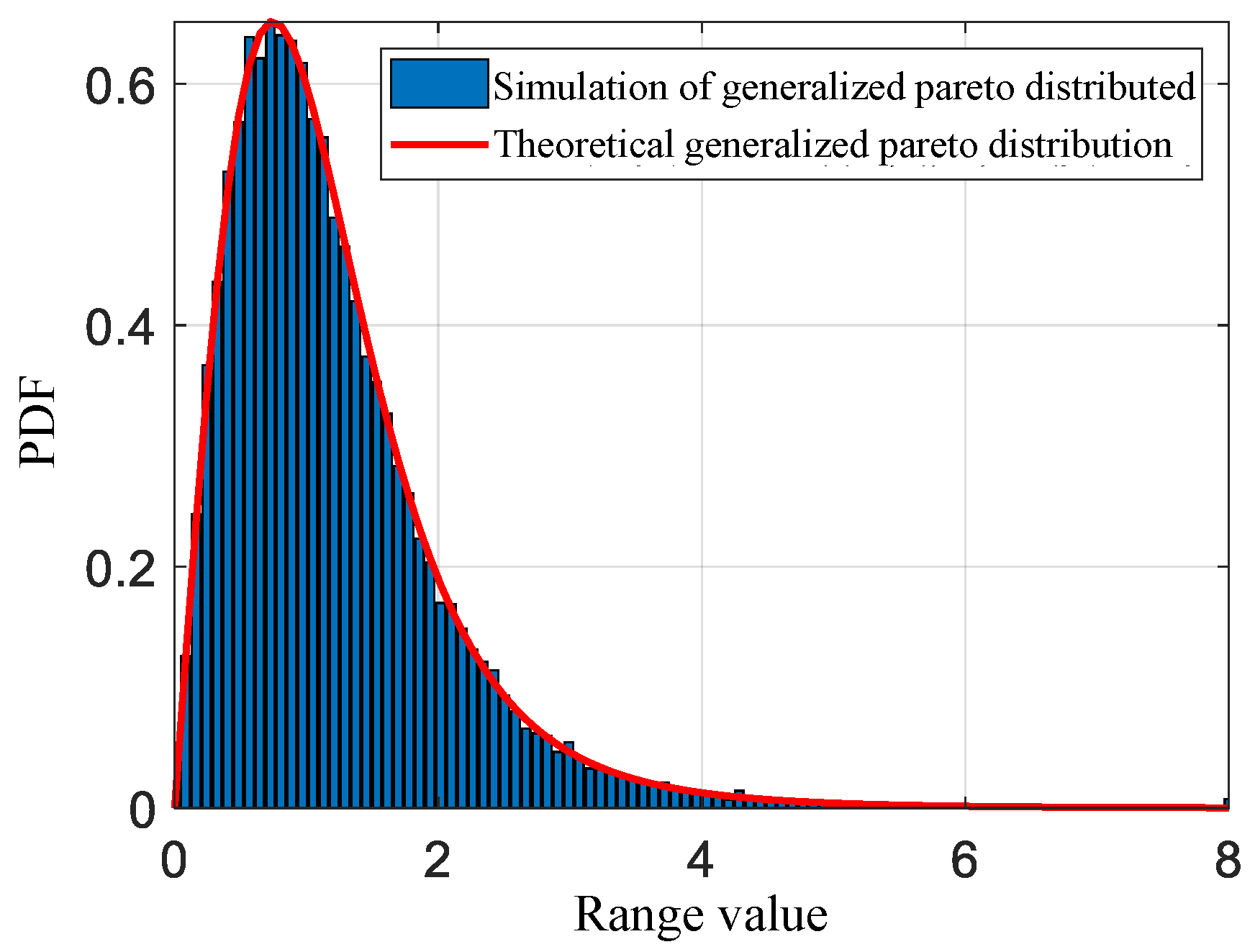
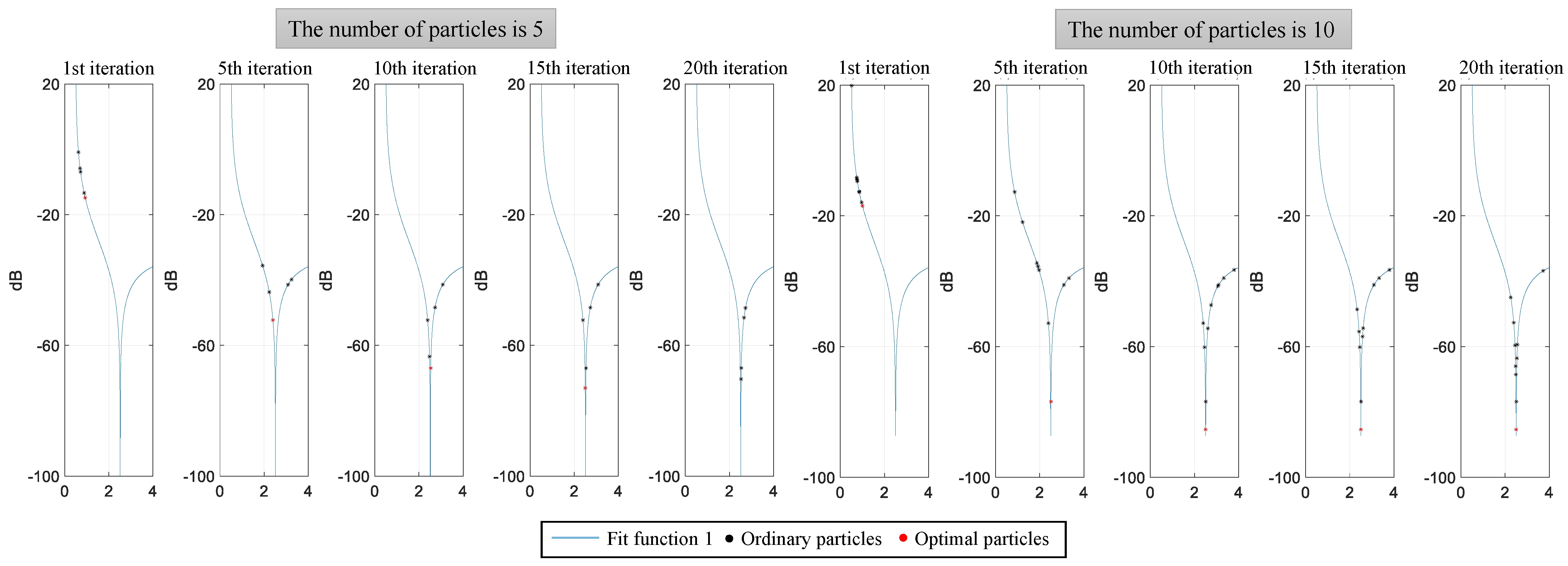
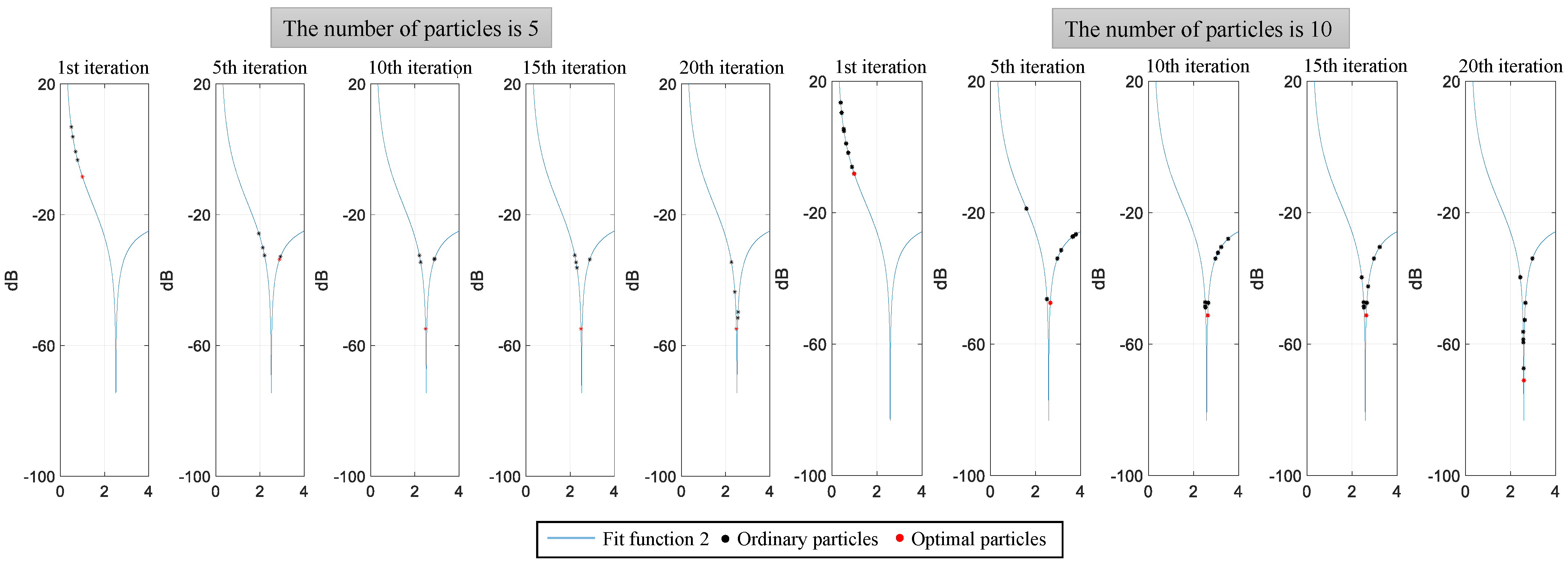
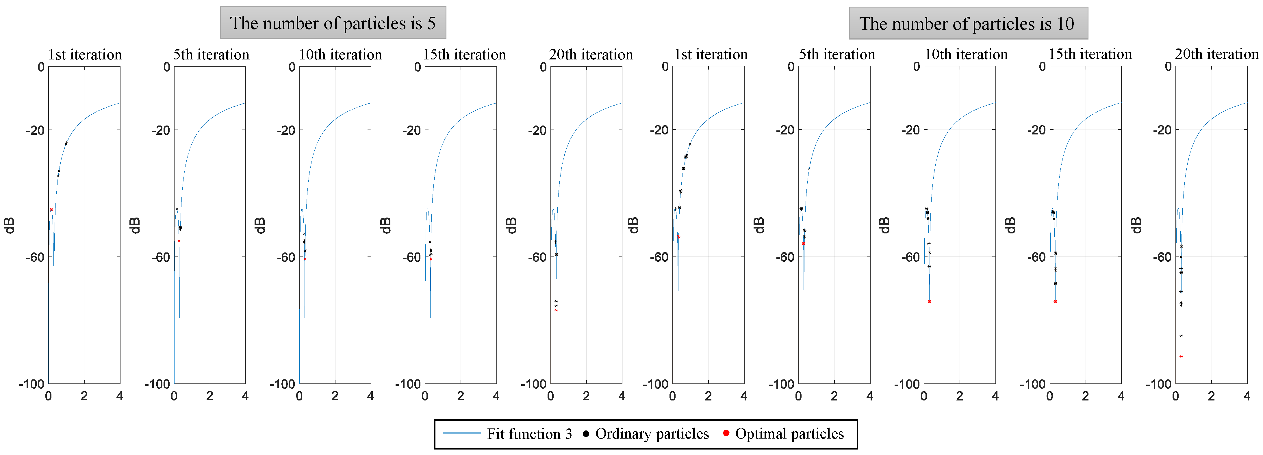
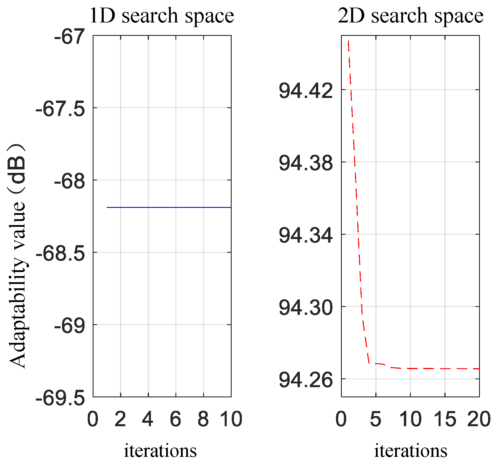
• By using simulated random data samples of the generalized Pareto distribution, the impact of parameters such as population size and iteration count in the PSO algorithm on its performance is examined, and the optimal parameter configuration for each targeted objective is determined.
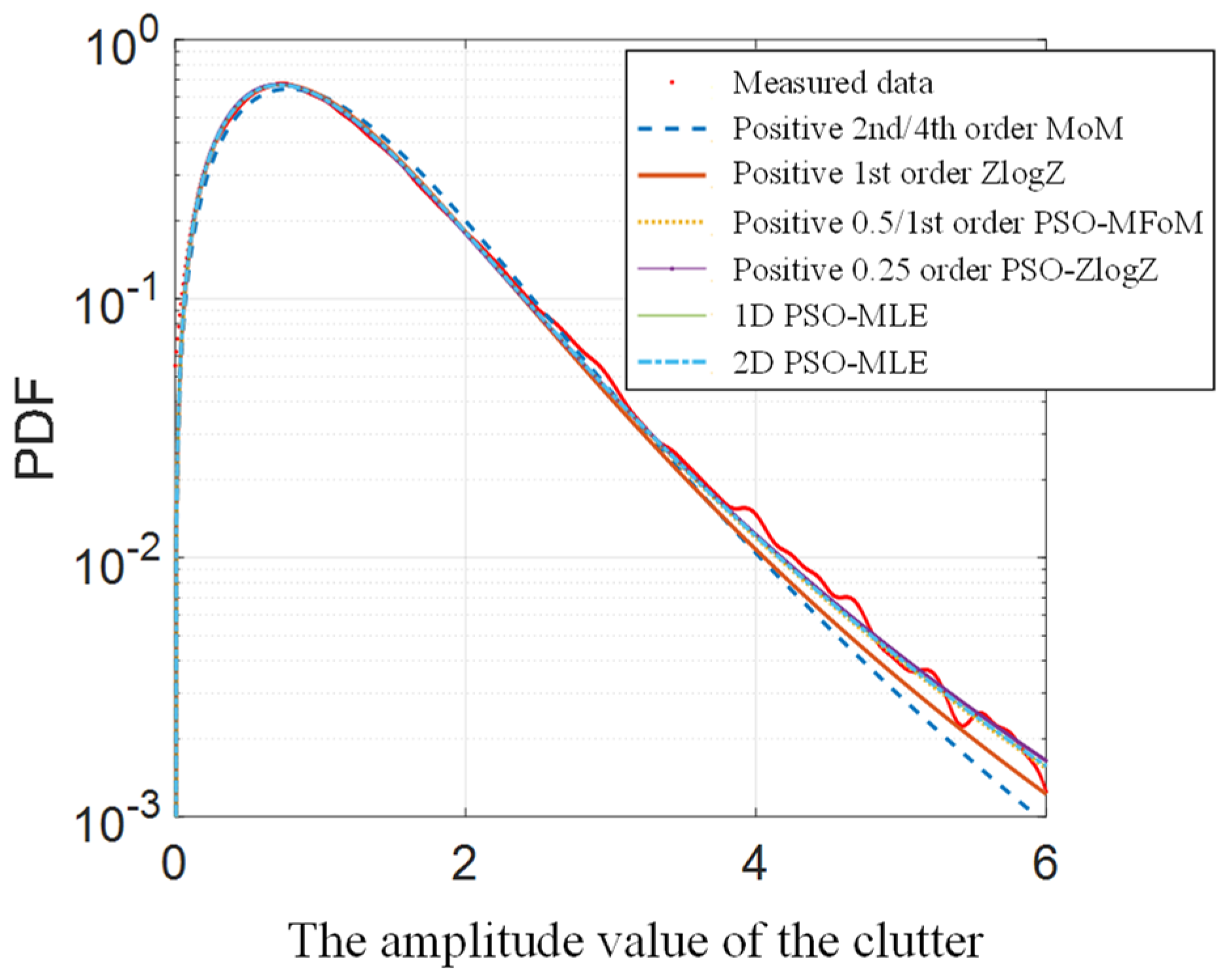
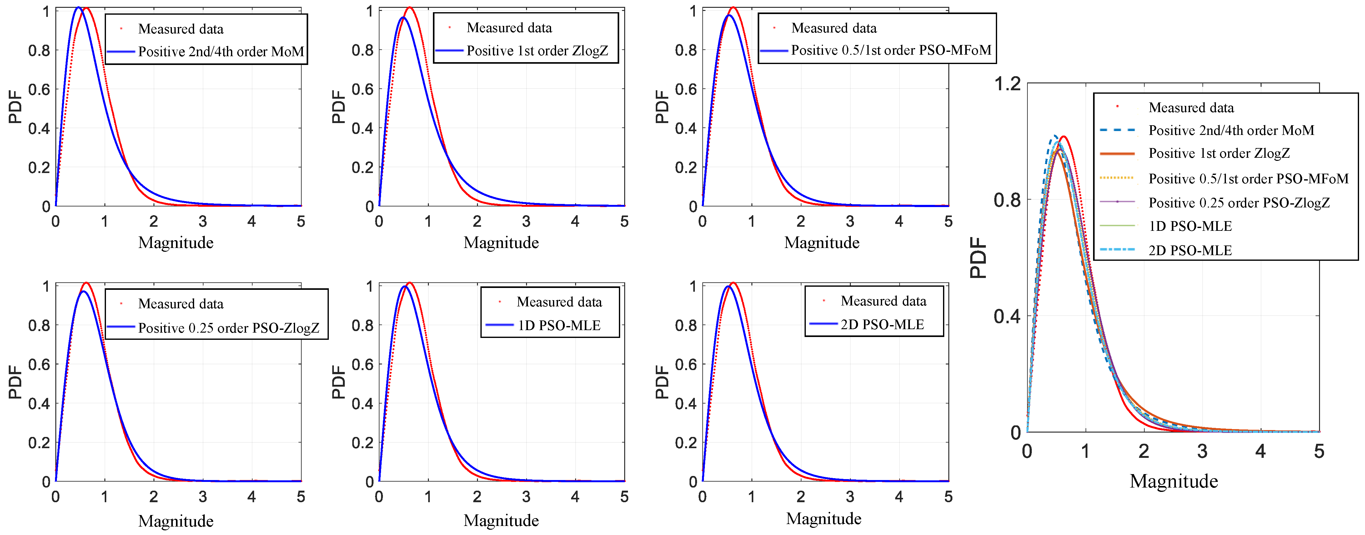
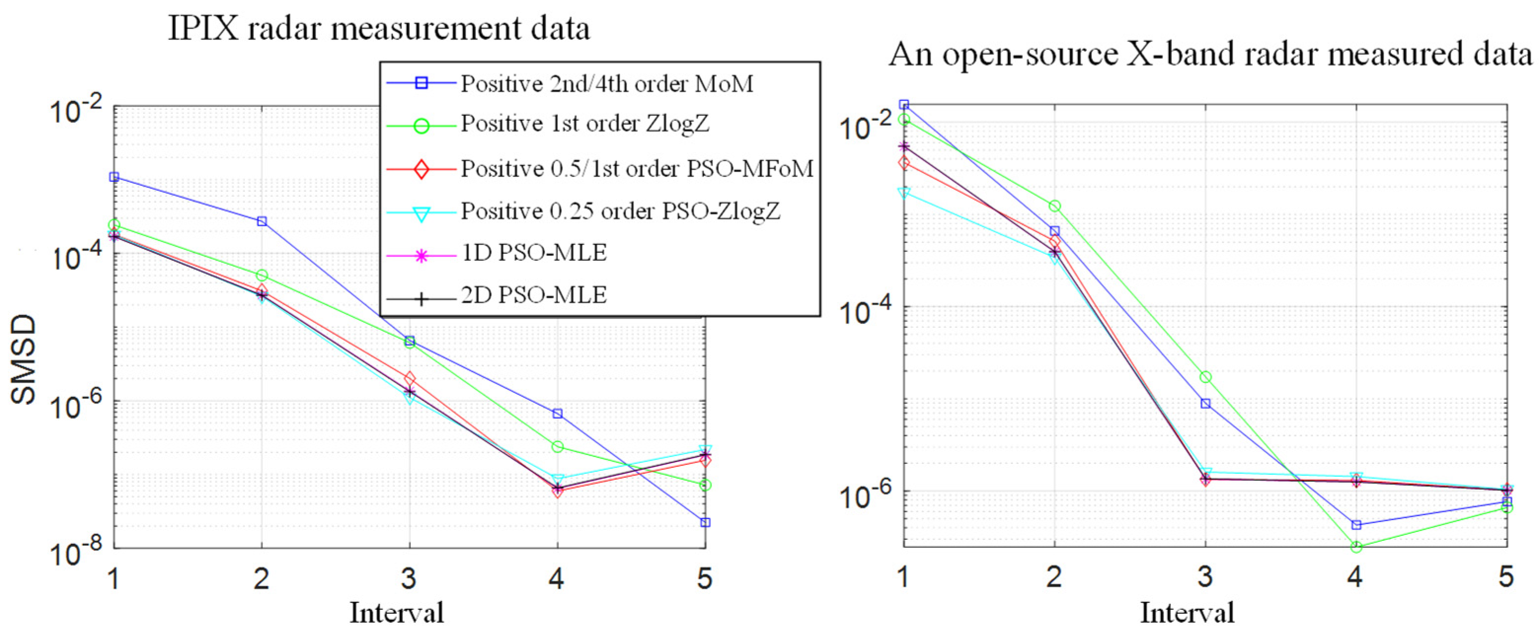
• A goodness-of-fit test experiment is conducted on two sets of high-intensity ocean wave clutter measured data to compare the fitting performance of the generalized Pareto distribution models obtained through different parameter estimation methods.
• The performance of the HPSO algorithm and the PSO algorithm is compared using simulated data based on the parameter estimation fitness function constructed in this study.

The experimental results demonstrate that the PSO algorithm not only expands the parameter estimation range of the generalized Pareto distribution but also significantly improves its fitting performance to observed data, particularly in the case of heavy-tailed ocean clutter data. Furthermore, simulation experiments reveal that the HPSO algorithm outperforms the PSO algorithm when it comes to solving the task of optimal parameter search for the generalized Pareto distribution.

The remaining sections of the paper are organized as follows. Section 2 provides background information on the generalized Pareto distribution model and its fundamental parameter estimation techniques. In Section 3, we present a comprehensive explanation of the parameter estimation methods for the generalized Pareto distribution model, with a specific focus on the PSO-based approach and the proposed HPSO method. Section 4 presents the experimental results, followed by analysis and discussion. Finally, in Section 5, we present the conclusions drawn from our findings and discuss potential avenues for future research.

2. Background

In this section, we briefly introduce the necessary background of the generalized Pareto distribution model and its basic parameter estimation methods.

2.1. Generalized Pareto Distribution Model

The generalized Pareto distribution is a kind of composite Gaussian model, which is widely used in the statistical modeling of sea clutter data of high-resolution sea-going radar [30]. The composite Gaussian model is formed by a random process modulating an independent distribution, which can be expressed as the result of the slow-varying structural component $\tau$ modulating the fast-varying scattering component $\mu$. In the study of the backscattering mechanism at the sea surface [31], it is known that the structural component is formed by the large-scale steep wave crests and white caps in the sea surface structure, while the scattering component is mainly composed of the small-scale tension waves and surges at the sea surface. The mathematical form of the above stochastic process is as follows:

$$c\left(t\right)=\sqrt{\tau \left(t\right)}\mu \left(t\right),\hspace{1em}\hspace{1em}t=1,2,\cdots$$

(1)

where the scattered component $\mu$ is a complex Gaussian random variable with zero mean and unit covariance, the structural component $\tau$ is a positive random process obeying the inverse gamma distribution, i.e., $1/\tau$ satisfies the gamma distribution, and the probability density function is defined as

$$f_{\tau }\left(\tau ;a,b\right)=\frac{1}{b^a\Gamma \left(a\right)}{\tau }^{-\left(a+1\right)}{e}^{-\frac{1}{b\tau }}$$

(2)

where a is the shape parameter, reflecting the dragging degree of the statistical distribution of sea clutter data, the larger the shape parameter a, the more obvious the dragging phenomenon; b is the scale parameter, characterizing the intensity level of the echo signal. According to the product form of two random processes in Equation (1), the amplitude probability density function (PDF) of the generalized Pareto distribution can be deduced as

$$f_x\left(x\right)={\displaystyle {\int }_0^{\infty }{f}_{\tau }}\left(\tau ;a,b\right)f_{\mu }\left(x|\tau \right)\mathrm{d}\tau$$

(3)

where $f_{\tau }(x|\tau )$ is the PDF of the scattered component $\mu$, which has the following mathematical expression:

$$f_u\left(x|\tau \right)=\frac{2x}{\tau }{e}^{\frac{-x^2}{\tau }}$$

(4)

Substituting Equations (2) and (4) into Equation (3) above, the following generalized Pareto distribution magnitude PDF derivation can be obtained:

$$\begin{array}{cc}{f}_x\left(x\right)& ={\displaystyle {\int }_0^{\infty }\frac{1}{b^a\Gamma \left(a\right)}{\tau }^{-\left(a+1\right)}{e}^{-\frac{1}{b\tau }}}\frac{2x}{\tau }{e}^{\frac{-x^2}{\tau }}\mathrm{d}\tau \\ & =\frac{2xb}{{\left(1+b{x}^2\right)}^{a+1}\Gamma \left(a\right)}{\displaystyle {\int }_0^{\infty }{y}^a{e}^{-y}\mathrm{d}y}\\ & =\frac{2xab}{{\left(1+b{x}^2\right)}^{a+1}}\end{array}$$

(5)

where the variable x is replaced by $y=\left(1+b{x}^2\right)/b\tau$. In addition, when the structural component in Equation (3) is in the form of an exponential distribution, the intensity distribution of the generalized Pareto distribution can be deduced as

$$p\left(x\right)=\frac{ab}{{\left(1+bx\right)}^{\left(a+1\right)}}$$

(6)

From the above Equation (5), it can be seen that the amplitude PDF of the generalized Pareto distribution approximates the Rayleigh distribution when the shape parameter $a\to \infty$, and the sea clutter amplitude trailing phenomenon is gradually aggravated when $a\to 0$. The fixed scale parameter b, the variation of the amplitude PDF curve of the generalized Pareto distribution with the shape parameter a, is shown in Figure 1. As can be seen from Figure 1, when the scale parameter b is fixed to 1.5, the wave crest of the amplitude PDF curve of the generalized Pareto distribution increases with the increase in the shape parameter, the wave crest gradually moves in the direction of smaller amplitude, and the trailing becomes shorter.

2.2. Basic Parameter Estimation Methods for the Generalized Pareto Distribution

The most critical step in the practical application of the generalized Pareto distribution for modeling the statistical properties of sea clutter is to achieve accurate parameter estimation and to improve the detection performance of sea radar. For different distribution models, a robust parameter estimation method is the basis for the application of the distribution model. The commonly used parameter estimation methods include moment estimation class methods, maximum likelihood estimation methods, quantile parameter estimation methods, and artificial intelligence class parameter estimation methods.

Among the moment estimation class methods, both positive 2nd/4th-order moment estimation and 1st-order logarithmic moment estimation have closed expressions for parameter estimation, which can easily obtain the results of parameter estimation, but are limited by the estimation range of shape parameters. The positive 0.5th/1st-order moment estimation extends the estimation range of the shape parameter to the fractional domain, but the method does not have a closed expression. The positive 0.25th-order logarithmic moment estimation method can achieve a further extension of the shape parameter, thus widening the space where the generalized Pareto distribution should be used in the statistical modeling of sea clutter, but the method also cannot derive a closed parameter estimation expression. The maximum likelihood estimation can obtain a relatively high accuracy of parameter estimation, but the parametric results of the scale parameters are given by a nonlinear system of equations, which again does not have a displayed solution. In the following, the mathematical forms of each type of parameter estimation method introduced above will be derived one by one and used as the basis for the optimization of parameter estimation of the generalized Pareto distribution later.

The method of moment estimation class parameter estimation equates the moments of each order of the probability distribution model of the sample to the cumulants of the statistical distribution model and obtains all parameter values of the distribution model by solving the system of moment equations of each order. Assuming the unknown parameter $\theta =\left(a,b\right)$ of the generalized Pareto distribution, the r-th-order moments of the origin of the probability density function can be calculated from Equation (5) as

$$\begin{array}{cc}E\left(x^r\right)& ={\displaystyle {\int }_0^{\infty }{x}^{r}f\left(x;\mathit{\theta }\right)}\mathrm{d}x,\left\{r\in R \mathrm{and} r\ne 0\right\}\\ & ={\displaystyle {\int }_0^{\infty }\frac{2ab{x}^{r+1}}{{\left(1+b{x}^2\right)}^{\left(a+1\right)}}}\mathrm{d}x=\frac{a}{b^{\frac{r}{2}}}{\displaystyle {\int }_0^{\infty }\frac{{\lambda }^{r/2}}{{\left(1+\lambda \right)}^{\left(a+1\right)}}}\mathrm{d}\lambda \\ & =\frac{1}{b^{r/2}}\frac{\Gamma \left(1+\frac{r}{2}\right)\Gamma \left(a-\frac{r}{2}\right)}{\Gamma \left(a\right)}\end{array}$$

(7)

where the variable $\lambda =b{x}^2$, the solution process involves some of the relevant properties of the gamma function operation, and it is known from its properties that the above equation needs to satisfy $a>r/2$ to hold, i.e., the estimation range of the shape parameter will be limited. If the sea clutter sample data $\mathit{X}=\left[x_1,x_2,\cdots ,x_n\right]$ are known, the r-th-order sample origin moment of the random data $\mathit{X}$ is $m_r=1/n{{\displaystyle \sum }}_1^n{x}_i^r$. The generalized Pareto distribution contains two parameters to be estimated, so it is necessary to list the equations of two different order moments and complete the equation solution to obtain the determined distribution model.

When r is taken as 2 and 4, respectively, the parameter estimation expression for positive 2nd/4th-order moment estimation is:

$$\{\begin{array}{l}\widehat{a}=2+\frac{2m_2^2}{m_4-2m_2^2}\\ \widehat{b}=\frac{1}{\left(\widehat{a}-1\right)m_2}\end{array}$$

(8)

When r is taken as 0.5 and 1, respectively, the parameter estimation expression for positive 0.5th/1st-order moment estimation is:

$$\{\begin{array}{l}\frac{\Gamma \left(\widehat{a}-0.5\right)\Gamma \left(\widehat{a}\right)}{{\Gamma }^2\left(\widehat{a}-0.25\right)}=\frac{{\Gamma }^2\left(1.25\right)m_1}{\Gamma \left(1.5\right)m_{0.5}^2}\\ \widehat{b}=\left(\frac{\Gamma \left(1.5\right)\Gamma \left(\widehat{a}-0.5\right)}{\Gamma \left(\widehat{a}\right)m_1}\right)\end{array}$$

(9)

The above Equation (8) can be obtained by substituting the calculated sample 2nd- and 4th-order moments of origin into the set of equations to obtain the estimation results of the parameters. From Equation (9), it can be seen that there is no closed expression for the estimation of the shape parameters, so the parameter estimation results cannot be calculated directly by substituting the values of the sample moments.

In addition, the method of estimating log moments of the generalized Pareto distribution proposed in the literature [32] also belongs to the moment estimation class of parameter estimation methods, assuming $Z=x^2$, then the r-th-order origin moments of the intensity probability density function of the generalized Pareto distribution and the corresponding sample moments can be defined as

$$\{\begin{array}{l}E\left(z^r\right)={\displaystyle {\int }_0^{\infty }{z}^r\ln z\cdot p}\left(z;\mathit{\theta }\right)\mathrm{d}z\\ {\kappa }_r=\frac{1}{n}{\displaystyle \sum _{i=1}^n{z}_i^r}\ln z_i\end{array},r\in R$$

(10)

Replacing the overall moment with the sample moment in Equation (10) yields

$$\{\begin{array}{l}\frac{{\kappa }_r}{m_{2r}}-{\kappa }_0=\psi \left(1+r\right)-\psi \left(1\right)+\psi \left(\widehat{a}\right)-\psi \left(\widehat{a}-r\right)\\ \hspace{1em}\widehat{b}=\exp \left(\psi \left(1\right)-{\kappa }_0-\psi \left(a\right)\right)\end{array}$$

(11)

where $\Psi (·)$ is the digamma function, which is obtained by taking the logarithm of the gamma function and then deriving it, and satisfies $\Psi \left(1+x\right)=\Psi \left(x\right)+1/x$. By the nature of the digamma function, it is known that the effective estimation range of the shape parameter is $a>r$.

When r is equal to 1, the parameter estimation expression for positive 1st-order logarithmic moment estimation is

$$\{\begin{array}{l}\widehat{a}=1+\frac{1}{{\kappa }_1/m_2-{\kappa }_0-1}\\ \widehat{b}=\exp \left(\psi \left(1\right)-{\kappa }_0-\psi \left(\widehat{a}\right)\right)\end{array}$$

(12)

The positive 1st-order logarithmic moment estimation exists for the displayed solution, and the parameter estimation can be obtained by calculating the logarithmic moment and the integer order moment values of the corresponding order of the sample and then substituting them into Equation (12).

When r is equal to 0.25, the logarithmic moment estimation corresponds to the positive 0.25th-order logarithmic moment estimation method, and it can be seen from Equation (11) that the shape parameter estimator does not have a closed expression at this time, and the parameters cannot be solved directly through the substitution of sample moments.

Maximum likelihood estimation is a relatively common parameter estimation method with specific applications in the estimation of parameters of various types of statistical distribution models. The method has a relatively high accuracy of parameter estimation and is close to the lower bound of what can be achieved in terms of parameter estimation accuracy. The log-likelihood function of the generalized Pareto distribution is as follows:

$$\begin{array}{ll}L\left(a,b\right)& =\ln {\displaystyle \prod _{i=1}^n{f}_x\left(x_i;a,b\right)}=\ln \left[{\left(2ab\right)}^n{\displaystyle \prod _{i=1}^n\frac{x_i}{{\left(1+b{x}_i^2\right)}^{a+1}}}\right]\\ & =n\ln \left(2ab\right)-{\displaystyle \sum _{i=1}^n\left(a+1\right)\ln \left(1+b{x}_i^2\right)+{\displaystyle \sum _{i=1}^n\ln x_i}}\end{array}$$

(13)

To find the optimal parameters when the log-likelihood function is maximized, Equation (13) is derived for the generalized Pareto distribution for the shape parameter a and the scale parameter b, respectively, and the derivative is set to zero, resulting in the following equation of the likelihood function:

$$\{\begin{array}{c}\frac{\partial L\left(a,b\right)}{\partial a}=\frac{n}{a}-{\displaystyle \sum _{i=1}^n\ln \left(1+b{x}_i^2\right)=0}\\ \frac{\partial L\left(a,b\right)}{\partial b}=\frac{n}{b}-\left(a+1\right){\displaystyle \sum _{i=1}^n\frac{x_i^2}{b{x}_i^2+1}=0}\end{array}$$

(14)

By eliminating the scale parameter b in the above set of equations through covariance substitution, the maximum likelihood function estimator of the shape parameter a can be obtained, and it is re-substituted into Equation (14) to obtain the estimator of the scale parameter. The maximum likelihood estimator of the generalized Pareto distribution is as follows:

$$\{\begin{array}{l}\widehat{a}=\frac{n}{\widehat{b}{\displaystyle \sum _{i=1}^n\frac{x_i^2}{1+\widehat{b}{x}_i^2}}}-1\\ \frac{1}{n}{\displaystyle \sum _{i=1}^n\ln \left(1+\widehat{b}{x}_i^2\right)}\left(1-\frac{1}{n}{\displaystyle \sum _{i=1}^n\frac{\widehat{b}{x}_i^2}{1+\widehat{b}{x}_i^2}}\right)=\frac{1}{n}{\displaystyle \sum _{i=1}^n\frac{\widehat{b}{x}_i^2}{1+\widehat{b}{x}_i^2}}\end{array}$$

(15)

where the calculation of the shape parameter $\widehat{a}$ needs to obtain the value of the scale parameter $\widehat{b}$ first, but the parameter $\widehat{b}$ cannot be obtained directly through calculation, and the corresponding objective function can be established, and then the optimal value can be obtained by searching for the optimal value.

The basic parameter estimation methods of the generalized Pareto distribution are introduced above, the characteristics of various estimation methods are explained, specific parameter estimation expressions are given, and

Table 1. Feature comparison of parameter estimation methods.

Parameter Estimation Methods	Shape Parameter Estimated Range	Estimated Expressions
Positive 2nd/4th-order moment estimation (MoM)	(2, +∞)	Closure
Positive 0.5th/1st-order moment estimation (MfoM)	(0.5, +∞)	Non-closed
Positive 1st-order logarithmic moment estimation ()	(1, +∞)	Closure
Positive 0.25th-order logarithmic moment estimation (Zlogz)	(0.25, +∞)	Non-closed
Maximum Likelihood Estimation (MLE)	(0, +∞)	Non-closed

shows the comparison of the characteristics of each parameter estimation method.

As can be seen from Table 1, some of the parameter estimation methods for the generalized Pareto distribution have expressions that are non-closed, and to obtain parameter estimation results for such parameter estimation methods, intelligent algorithms can be used to solve the parameter estimation problem for non-closed expressions. All the non-closed expressions involved in the table are nonlinear functions, so they can be transformed into a nonlinear function of the optimization problem.

The intelligent algorithm itself has nonlinear characteristics, and a suitable intelligent algorithm can be used to complete the search for the optimal solution of the nonlinear function in the target feasible solution space in order to obtain the estimated values of the non-closed expressions in the parameter estimation method of the partial generalized Pareto distribution.

3. Method

3.1. Particle Swarm Optimization Algorithm

The particle swarm optimization (PSO) algorithm is a swarm intelligence class optimization algorithm that originated from the study of bird predation behavior, which was proposed by Kennedy and Eberhart in 1995 [33] and has been widely used in many fields after more than a decade of continuous research and development [34,35]. The PSO algorithm randomly initializes particles in the feasible solution space of the problem, and each particle is given a certain velocity of motion at its initial position, and the trajectory of the particles is influenced by its factors and the overall behavior of the population during the whole iteration cycle.

The fitness function is the target object of the particle population activity because it determines the activity space and search path of the particles. The particle population has the ability of memory, and all particles calculate the corresponding fitness value in each iteration, then compare it with the historical value and select the optimal value of the historical record, and then guide the whole population toward the direction of the global optimal solution. The basic process of the particle swarm algorithm is:

(a)

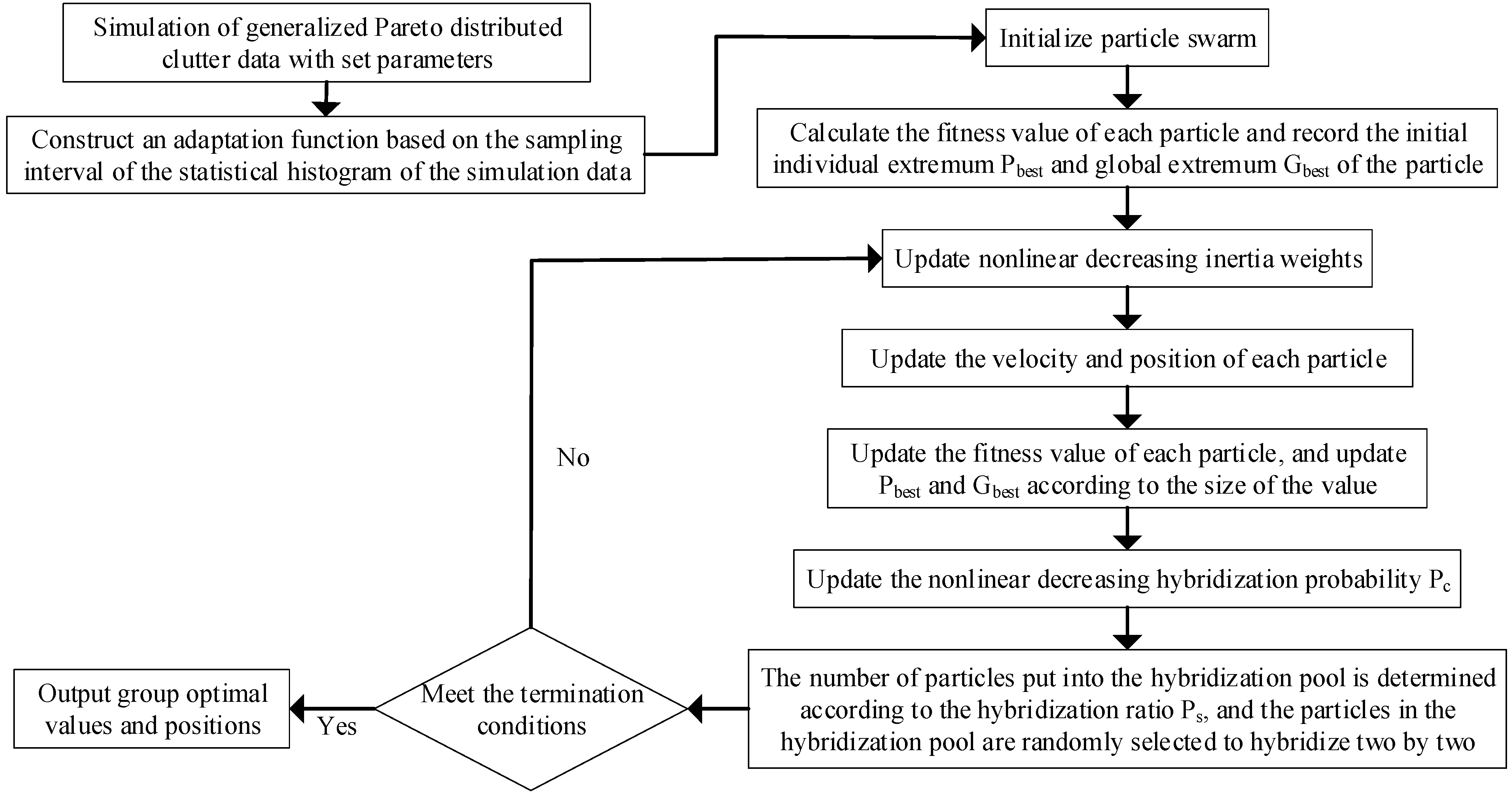
The positions X and velocities V of the particles are randomly initialized in the D-dimensional space of feasible solutions, where the i-th particle position and velocity can be expressed as

$$\{\begin{array}{c}{\mathit{X}}_i=\left(x_{i1},x_{i2},\cdots ,x_{iD}\right)\\ {\mathit{V}}_i=\left(v_{i1},v_{i2},\cdots ,v_{iD}\right)\end{array},i=1,2,\cdots ,N$$

(16)

(b)

Based on the determined fitness function (particle population search object) and the corresponding position of each particle, the corresponding fitness value is calculated, and then the global optimum is evaluated, where the historical optimum of the particle and the global optimum of the population is assumed to be $P_{best}$ and $G_{best}$, respectively, that is, we have

$$\{\begin{array}{c}{\mathit{P}}_{best}=\left(p_{1i},p_{2i},\cdots ,p_{iD}\right)\\ {\mathit{G}}_{best}=\left(g_{1i},g_{2i},\cdots ,g_{iD}\right)\end{array},i=1,2,\cdots ,N$$

(17)

(c)

The particle population is continuously updated iteratively to search for the extreme value solution of the fitness function, and the velocity and position of each particle in the next iteration are updated by the individual historical optimal value $P_{best}$ and the current velocity V_i, and the k + 1th update of the particle is given by

$$\begin{gathered} V_{id}^{k+1}=\omega V_{id}^k+c_1{r}_1\left(P_{id}^k-X_{id}^k\right)+c_2{r}_2\left(P_{gd}^k-X_{id}^k\right) \\ {X}_{id}^{k+1}=X_{id}^k+V_{id}^{k+1} \end{gathered}$$

(18)

where w is the inertia weight, which gives the particle the inertia of motion trend; k is the number of current iterations; $c_1$ and $c_2$ are learning factors; and $r_1$ and $r_2$ are random numbers distributed in the interval of [0, 1]. To prevent the particles from searching blindly and falling into the risk of local optimum, the velocity and position of the particles are usually limited to a certain interval. The learning factor and inertia weight are particularly important parameters of the PSO algorithm, where the learning factor $c_1$ of the particle itself, also known as the cognitive parameter, is an important indicator of the particle’s search ability; the learning factor $c_2$ of the population is a social cognitive parameter that affects the search behavior of the whole particle population; and the size of the inertia weight is an expression of the movement ability of each particle.

(d)

Finally, the algorithm is terminated by setting the corresponding end conditions. There are generally two kinds of termination conditions: the first is to set the maximum number of iterations of the particle population, and the second criterion is to terminate when the optimal solution of the particle swarm has remained unchanged for five or more consecutive iterations.

The most critical issue in the practical application of particle swarm algorithms is to balance the relationship between particle search capability and algorithm performance and parameters.

3.2. Parameter Estimation Based on PSO Algorithm

When running a PSO algorithm, the setting of parameters such as learning factors and inertia weights has a very important impact on the optimal solution of the algorithm for a particular problem [36,37]. The combination of different parameters of the PSO algorithm causes the particle population to form different trajectories and affects the searchability of the particles. For the specific search problem, it is necessary to choose the appropriate combination of algorithm parameters, and in this paper, it is necessary to solve the problem of solving the non-closed expressions for the generalized Pareto distribution with positive 0.5th/1st-order moment estimation, positive 0.25th-order logarithmic moment estimation, and maximum likelihood estimation. Therefore, for the above discussion, this paper will use the appropriate combination of parameters to complete the solution of the corresponding target problem.

To address the problem of solving non-closed expressions in the parameter estimation methods of generalized Pareto distribution, the whole thought process of the PSO algorithm introduced to solve this problem is introduced in detail, including the construction of the fitness function and the setting of algorithm parameters. According to the derivation in Section 2, it is known that the positive 0.5th/1st-order moment estimation, positive 0.25th-order logarithmic moment estimation, and maximum likelihood estimation have non-closed expressions, so the fitness functions of the three types of estimation methods are constructed as follows:

$$\{\begin{array}{l}{f}_1\left(a\right)=\frac{\Gamma \left(a-0.5\right)\Gamma \left(a\right)}{{\Gamma }^2\left(a-0.25\right)}-\frac{{\Gamma }^2\left(1.25\right)m_1}{\Gamma \left(1.5\right)m_{0.5}^2}\\ f_2\left(a\right)=\frac{{\kappa }_{0.25}}{m_{0.5}}-{\kappa }_0-\psi \left(1.25\right)+\psi \left(1\right)-\psi \left(a\right)+\psi \left(a-r\right)\\ f_3\left(b\right)=\frac{1}{n}{\displaystyle \sum _{i=1}^n\ln \left(1+b{x}_i^2\right)}\left(1-\frac{1}{n}{\displaystyle \sum _{i=1}^n\frac{b{x}_i^2}{1+b{x}_i^2}}\right)-\frac{1}{n}{\displaystyle \sum _{i=1}^n\frac{b{x}_i^2}{1+b{x}_i^2}}\end{array}$$

(19)

In this case, the three fitness function constructions correspond to one-dimensional nonlinear function extremum search problems, and the final parameter estimates can be obtained as long as the particle population is made to find the location in the feasible solution space where the minimal value point is located.

3.3. Improved Parameter Estimation for Particle Swarm Hybridization

In the PSO algorithm, the inertia weight factor is a key parameter that affects the search capability, velocity, and search range of each particle in the solution space. In this section, we introduce a non-linearly decreasing inertia weight that varies with the number of iterations. The non-linearly decreasing inertia weight allows particles to have higher inertia in the initial stage, enhancing their global search capability. As particles approach the optimal position, the inertia weight decreases, restricting their movement to a smaller local range and improving search precision. The updated formula for the inertia weight is given as follows:

$$\omega \left(k\right)={\omega }_{start}-\left({\omega }_{start}-{\omega }_{end}\right){\left(\frac{k}{N_{\max }}\right)}^2$$

(20)

where ${\omega }_{start}$ represents the initial inertia weight, and ${\omega }_{end}$ represents the inertia weight at the maximum number of iterations. $k$ represents the current iteration number, and $N_{max}$ represents the maximum number of iterations. The PSO algorithm suffers from the problem of premature convergence, where particles becomes trapped in local optima, thereby affecting the convergence accuracy of the algorithm. To address this issue, we introduce the selection and recombination operations from genetic algorithms into the PSO algorithm, referred to as the HPSO algorithm. This approach significantly improves the problem of premature convergence in the population. After updating the positions and velocities of all particles, a certain number of particles are selected for recombination based on the hybrid pool size ratio $P_s$. With a given recombination probability $P_c$, two particles are randomly selected and undergo recombination, and the resulting offspring particles replace the parent particles. This process helps particles escape from local optima. The recombination formula for parent particles is as follows:

$$\begin{array}{l}child\left(x\right)=P_c\ast paren{t}_1\left(x\right)+\left(1-P_c\right)\ast paren{t}_2\left(x\right)\\ child\left(v\right)=\frac{paren{t}_1\left(v\right)+paren{t}_2\left(v\right)}{\left|paren{t}_1\left(v\right)+paren{t}_2\left(v\right)\right|}\left|paren{t}_1\left(v\right)\right|\end{array}$$

(21)

where parent (x) and parent (v) represent the position and velocity of the hybrid particles, while child (x) and child (v) represent the position and velocity of the offspring particles resulting from the hybridization process. When two particles trapped in different local optima undergo hybridization, they can escape from their respective local optima and improve the global search capability of the population. Additionally, if the hybrid particle group adopts a fixed hybridization probability $P_c$, it may result in repetitive and ineffective hybridization operations within the local range during the later iterations, leading to decreased algorithm efficiency and the loss of the advantages of hybridization. To address this issue, a nonlinearly decreasing hybridization probability is employed, where the hybridization probability of the parent particles decreases nonlinearly with the increase in iteration count. The updated formula for the hybridization probability $P_c$, is as follows:

$$P_c=\left(P_{c1}-P_{c2}\right){\left(1-\frac{k}{N_{\max }}\right)}^2+P_{c2}$$

(22)

where $P_{c1}$ represents the initial crossover probability and $P_{c2}$ represents the crossover probability at the maximum number of iterations. The introduction of a nonlinearly decreasing crossover probability enhances the global search capability of particles in the early iterations while addressing the issue of local search efficiency in the later iterations. The basic steps of the proposed HPSO algorithm in this study are as follows:

Step 1. Initialize the particle swarm, including the swarm size N, the inertia weight $\omega$ for particle updates, the learning factors $c_1$ and $c_2$, as well as parameters for crossover operations such as the crossover pool size ratio $P_s$ and the crossover probability $P_c$. Set the position X and velocity V of each particle using uniform distribution random numbers within a certain range.

Step 2. Compute the fitness value for each particle based on the objective function and store it in the variable $P_{id}$. Select the best fitness value among the particles and store it in the variable $P_{gd}$. The variables $P_{id}$ and $P_{gd}$, respectively, represent the fitness value of the particles and the fitness value of the best position in the population for the current iteration.

Step 3. Update the inertia weight factor $\omega$ using the nonlinearly decreasing Formula (20).

Step 4. Update the velocity and position of each particle using the current iteration’s inertia weight, learning factors, and other algorithm parameters, following Formula (18).

Step 5. Compute the fitness value for each particle in the current iteration and compare it with the particle’s personal best position. Update the variable $P_{id}$ based on the fitness value. Then, compare all updated $P_{id}$ values with the global best position, updating the swarm’s variable $P_{gd}$.

Step 6. Update the crossover probability $P_c$ using the nonlinearly decreasing Formula (22).

Step 7. Select a specified number of particles specified by $P_s$ and place them in the crossover pool. Randomly select two particles from the pool to participate in a crossover. Update the position and velocity of the resulting offspring using Formula (21). Crossover operations generate the same number of particles as the parent generation.

Step 8. Check whether the termination condition of the algorithm is met. If satisfied, stop the swarm search and save the global best position of the particles. Otherwise, return to Steps 3 to 7 to continue the search.

The HPSO algorithm provides two ways to terminate the particle swarm search. The first approach is to set a maximum number of iterations for the particles, while the second approach involves specifying the number of generations to maintain the global best particle. Since determining the maximum number of iterations depends on the nature of the objective function and particle activities exhibit inherent randomness during each iteration, this section adopts the method of setting the number of generations to retain the global best particle to ensure an effective search for the optimal position of the objective function.

Different parameters of the generalized Pareto distribution can describe the amplitude distribution characteristics of ocean clutter under different background environments. The shape and scale parameters are the main factors influencing the statistical characteristics curve of the generalized Pareto distribution. To achieve an accurate fit of the generalized Pareto distribution to clutter data, the statistical histogram of clutter data is compared with the cumulative error on the theoretical distribution curve, which serves as the objective function for optimizing the parameter estimation of the generalized Pareto distribution. Furthermore, to balance the fitting discrepancies between the probability density function (PDF) curve and the cumulative distribution function (CDF) curve of clutter data, an adapted fitness function is constructed by appropriately weighting and combining two discrepancy functions. The HPSO algorithm is then employed to perform the corresponding optimal parameter search task. The fitness function for the parameter estimation of the generalized Pareto distribution is defined as follows:

$$f_{fitness}\left(\mathit{\theta }\right)=\frac{1}{1+{\lambda }_1{\displaystyle \sum _{n=1}^N{\left(f\left(n;\mathit{\theta }\right)-h\left(n\right)\right)}^2+{\lambda }_2{\displaystyle \sum _{n=1}^N{\left(F\left(n;\mathit{\theta }\right)-H\left(n\right)\right)}^2}}}$$

(23)

where $f\left(n;\theta \right)$ and $F\left(n;\theta \right)$, respectively, denote the PDF and CDF of the generalized Pareto distribution. $h\left(n\right)$ and $H\left(n\right)$ represent the values of the clutter statistical histogram at the PDF and CDF curve sampling intervals. The weighting coefficients are set as ${\lambda }_1=0.8$ and ${\lambda }_2=0.2$ in the experiments conducted in this paper.

The parameters of the HPSO algorithm are configured as follows: the population size is set to 20, the learning factor is denoted as $c_1=c_2=2$, the hybrid pool size ratio is denoted as $P_s=0.5$, and the minimum number of generations to maintain the global best position is set to 15. The initial values of the non-linearly decreasing inertia weight and hybrid probability are both 0.9 and their ending values are set to 0.4. Additionally, the maximum number of iterations is denoted as $N_{max}$ and is set to 50. Figure 2 illustrates the flowchart of the HPSO algorithm optimizing the objective function for estimating the parameters of the generalized Pareto distribution.

For comparative analysis, the parameters of the PSO algorithm are set as follows: the population size is 20, the learning factor is denoted as $c_1=c_2=2$, the inertia weight is denoted as $\omega =0.4$, and the maximum number of iterations is set to 50.

4. Results and Discussion

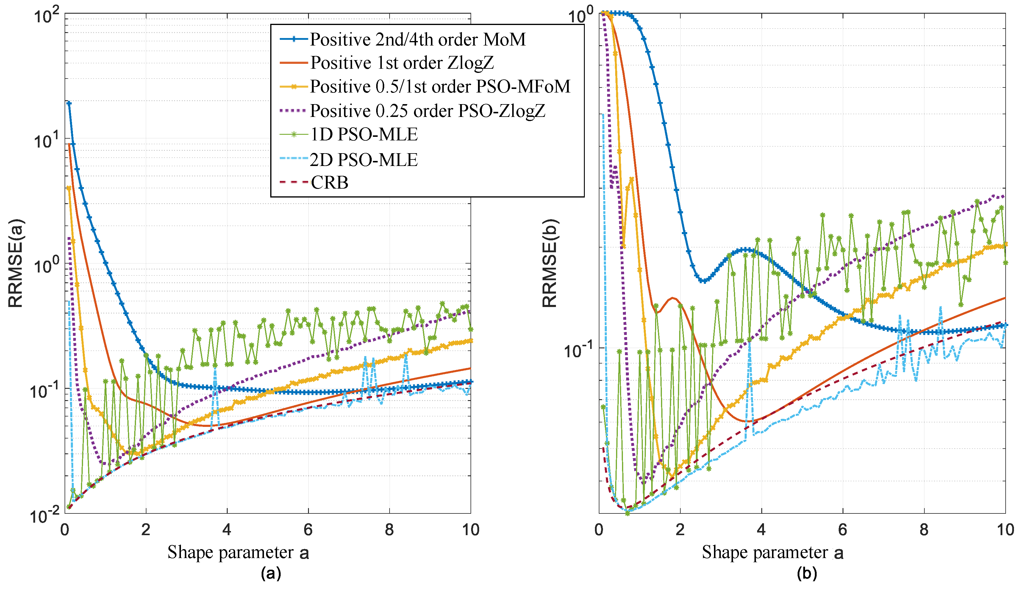
4.1. Simulation Experiment Analysis

The Monte Carlo method is used to generate random sequences obeying the generalized Pareto distribution. The parameters of the distribution model were set to a = 2.5, b = 0.3, and the length of the simulated data was 5 × 10⁴.

Figure 3 shows the statistical characteristics of the simulated data, from which it can be seen that the statistical characteristics of the simulated data match the theoretical distribution. To study the properties of the three fitness functions using the simulation data, various sample moments of the simulation data are calculated first, and then the results are substituted into Equation (19), that is, the curves of the fitness functions can be obtained as shown in Figure 4.

The fitness functions 1 and 2 correspond to the non-closed expressions for positive 0.5th/1st-order moment estimation and positive 0.25th-order logarithmic moment estimation, respectively. The fitness function 3 is significantly different from the first two functions because the horizontal coordinate of this function corresponds to the scale parameter domain and corresponds to the non-closed expression of the maximum likelihood estimate of the scale parameter. As can be seen from Figure 4, the range of values of the fitness functions 1 and 2 are both restricted to a certain space, [0.5, +∞] and [0.25, +∞], respectively, which must match the range of values of the shape parameters of the two-parameter estimation methods. The notches of the extreme value points of these three functions are relatively deep, so the particle population can quickly find the optimal location point during the search, but the number of inert particles increases sharply as the search process proceeds. The setting of the parameters of the PSO algorithm will determine the trajectory of the particles, and the influence of the number of particle populations and the number of iterations on the search behavior of the particle populations will be studied below.

According to the recommended values of optimal parameter settings given in the literature [37], the learning factors and inertia weights are set to $w=0.4, c_1=c_2=2$. To prevent the particles from crossing the boundary when searching, the particle population search space on the fitness functions 1 and 2 are restricted to [0.5, +∞] and [0.25, +∞], respectively, while the particle population search range of the fitness function 3 is restricted to [0.15, +∞]. The number of iterations is fixed to 20, and then the trajectories of each particle population at different numbers are observed separately, and the number of particles is set to 5 and 10, respectively. Figure 5, Figure 6 and Figure 7 give the positions of each particle in the first, 5, 10, 15, and 20 iterations for the three groups of particle populations, respectively.

All three particle populations search for the extremes of the fitness function in a one-dimensional space. The fitness functions 1 and 2 have similar curve shapes, so the same algorithm parameter settings can be used. As can be seen in Figure 5 and Figure 6, the deep notches in the curve of the fitness function allow the particles to move quickly to the vicinity of the extreme value point and thus determine the location of the optimal parameters. The increase in the number of particles and the number of iterations will lead to a longer algorithm operation time, but too few particles or insufficient iterations will easily make the particle population unable to complete the established search task, so the reasonable setting of the algorithm parameters is the key to successfully obtaining the optimal parameter estimation results of the distribution model. Too many particles reduce the efficiency of the algorithm while not bringing additional benefits to the population due to the increase in inert particles.

From Figure 7, it can be seen that with the increase in the number of iterations, the optimal particle of fitness function 3 appears to sink at the extreme value point. After analysis, it is found that there are infinitely many location points near the extreme value point, and the lowest valley shown in the figure is not the minimum of the curve, so the optimal particle will keep sinking. When the particle is near the notch, the difference in its corresponding horizontal coordinate position is already very small, so there is no need to make the particle sink into the deepest part of the notch after a large number of iterations. In the final experimental test, the number of particles and iterations of the three populations are set to 5 and 10, respectively, which meets the requirements of the particle population search task. The final algorithm parameter settings of this experiment can complete the search task for the optimal position of each fitness function in the shortest time.

The particle population search space determined by the fitness function 3 is theoretically within the whole positive real number domain, but the experimental test found that the particle movement to the position where the scale parameter is less than 0.15 results in a false-dead state, which causes the particle population to be trapped in this position all the time during the iterative process. After analysis, it is found that the possible reason for the above phenomenon is that the likelihood function, after taking logarithmic derivatives, limits the range of the scale parameter. To address this problem, we consider expanding the one-dimensional search space of the maximum likelihood function to two dimensions, i.e., directly searching the extremes of the maximum likelihood function in the space of scale parameters and shape parameters, thus skipping the step of taking logarithmic derivatives.

Figure 8 gives the iterative process of searching for the maximum likelihood function in different dimensions for the particle population. In which the one-dimensional space of the likelihood function, the search range of the particles is expanded from the original [0.15, +∞] to (0, +∞]. As a comparison, in the two-dimensional search space of the likelihood function, the search range of the particle population is also set to (0, +∞]. As can be seen from the figure, after expanding the search range of particles in the one-dimensional space, the particle population is initially trapped in an undefined position, making the particles inactive and falsely dead. The above phenomenon does not occur when the particle population is searched in the two-dimensional space of the likelihood function, and a higher accuracy of parameter estimation is obtained by searching directly in the two-dimensional space. Although the particle search in two dimensions can solve the problem of one-dimensional search, the expansion of the spatial search domain requires a larger number of particles and iterations to complete the search task, which undoubtedly increases the computational time complexity.

Table 2. Estimate time of each parameter estimation method.

Parameter Estimation Methods	MoM (2nd/4th-Order)	ZlogZ (1st-Order)	PSO-MFoM (0.5th/1st-Order)	PSO-ZlogZ (0.25th-Order)	PSO-MLE (1D)	PSO-MLE (2D)
Time/s	2.43 × 10−2	8.94 × 10−3	3.02 × 10−2	3.66 × 10−2	8.51 × 10−2	9.37 × 10−1

lists the time consumed by each parameter method of the generalized Pareto distribution.

From the data in Table 2, it can be seen that the parameter estimation of positive 1st-order logarithmic moments is the most efficient, and the parameter estimation time of positive 0.5th/1st-order moment estimation, positive 0.25th-order moment estimation, and maximum likelihood estimation based on the swarm subgroup optimization to solve the non-closed expression is comparable to that of positive 2nd/4th-order moment estimation; so the introduction of the particle swarm search does not significantly increase the computational time complexity of the parameter estimation method itself. The two-dimensional space search of the maximum likelihood estimation method doubles its computation time compared to the one-dimensional space, which is also consistent with the previous analysis. The operational efficiency of the algorithm is particularly important in applications with real-time processing, and the various advantages and disadvantages can be weighed in choosing a specific parameter estimation method based on the above discussion, which leads to the selection of a suitable parameter estimation method.

The estimation ranges of shape parameters for each parameter estimation method are detailed in Section 2. Here, to investigate the effect of shape parameters on the parameter estimation performance, we fixed the sample length of the simulation data at 10⁴, and the scale parameter b was set to 0.3. The estimation performance of the two-parameter model was then calculated by varying the shape parameter a from 0.1 to 10 in equal intervals. The results were evaluated using the relative root mean square error (RRMSE). Figure 9 shows the results of this experiment, where the specific calculation of the Cramér–Rao bound (CRB) can be found in the literature [38], and the values of each parameter node in the figure are obtained from the calculation of 30 independent replications of the experiment.

Observing Figure 9a,b, it can be found that the parameter estimation results obtained using PSO for the one-dimensional likelihood function are unstable, exhibiting significant fluctuations with errors oscillating beyond 0.1. Conversely, the results obtained from the two-dimensional likelihood function space search show more stable parameter estimation performance, with the RRMSE smaller than 0.1, and it approaches the CRB lower bound, which is consistent with the previous analysis. The parameter estimation performance of the maximum likelihood estimation method is not limited by the range of the shape parameters, while other parameter estimation methods are to some extent limited by the range of the shape parameters, i.e., accurate estimation of the shape parameters can be achieved only within the specified range. When the shape parameter is small (corresponding to the heavy trailing phenomenon of sea clutter), the estimation of higher order moments (positive 2nd/4th- and positive 1st-order logarithmic moments in Figure 9) is affected by the cumulative error of the sample, which leads to the poor performance of its parameter estimation. In addition, the estimation performance of all parameter estimation methods decreases with the increase in shape parameters.

4.2. Analysis of the Fit of the Measured Data

To verify the fitting effect of the generalized Pareto distribution model on the statistical properties of heavy trailing sea clutter data and to analyze the adaptability of different parameter estimation methods for parameter estimation of real data, this section performs a goodness-of-fit analysis on the statistical properties of a set of high-intensity data from the IPIX radar dataset [39,40] and an X-band radar open-source dataset [41,42], respectively.

Many scholars have carried out a large amount of research work on the perception of sea clutter properties based on the IPIX radar dataset, so this dataset is very reliable for the goodness-of-fit analysis. The effect of the distribution model on the sea clutter amplitude PDF fit is shown in Figure 10, and the two-parameter estimates of sea clutter data obtained via different parameter estimation methods are given in

Table 3. Estimation results of different parameter estimation methods.

Estimation Method	IPIX Radar Measurement Data						An X-Band Radar Open-Source Measurement Data
	MoM (2/4)	ZlogZ (1)	MFoM (05/1)	ZlogZ (0.25)	MLE (1D)	MLE (2D)	MoM (2/4)	ZlogZ (1)	MFoM (0.5/1)	ZlogZ (0.25)	MLE (1D)	MLE (2D)
Shape parameter	3.125	2.636	2.419	2.351	2.415	2.410	2.165	2.096	3.933	6.022	3.599	3.603
Scale Parameter	0.225	0.298	0.330	0.343	0.329	0.330	0.876	0.817	0.392	0.240	0.454	0.453

. Each dataset of the IPIX radar dataset contains 14 distance units, and a total of 131,702 data samples are collected for each distance unit. To reduce the running time, this experiment selects the non-target distance unit within (pure clutter data) 50,000 data samples, as the object of parameter estimation.

From Figure 10, it can be found that the PSO algorithm, compared to parameter estimation methods with explicit solutions, such as positive 2nd/4th-order and positive 1st-order logarithmic moments, not only effectively solves the problem of non-closed expressions in the three types of parameter estimation methods shown in the figure but also provides a distribution model that fits the heavy-tailed part of the observed data (with amplitudes in the range of 4–6) with a fitting distance smaller than 10⁻⁵.

Another X-band radar open-source sea clutter dataset is taken for parameter estimation experiments, and this dataset is obtained through the radar working in scanning mode to avoid the influence of near-coast land clutter background; only the data when the radar is scanning to the sea are intercepted for the goodness-of-fit analysis. Each set of data in this dataset contains 1320 distance units, and there are a total of 7369 samples within each distance unit. This experiment selected the clutter data from within distance units 801 to 810, and then intercepted the samples at each distance unit corresponding to the 501st to 3500th, for a total sample size of 30,000 (pure clutter data).

Figure 11 shows the fitting effect of the distribution model on the amplitude PDF of this group of data, and the two-parameter estimation results of this group of sea clutter data are shown in Table 3. It also reflects the fact that the particle swarm model introduced in this paper can fit the data. In addition, it also reflects that the problem of solving non-closed expressions for parameter estimation of the generalized Pareto distribution model has been effectively solved after the introduction of the particle swarm algorithm in this paper.

Both sets of experiments above observe the fitting effect of the distribution model directly from the plots. To quantitatively characterize the strengths and weaknesses of the fitting effect and then make a more accurate analysis of the fitting effect, the results of the Kolmogorov–Smirnov (K-S) test, the mean square deviation (MSD) test, and the root mean square deviation (RMSD) tests for the IPIX radar data and X-band radar open-source measured data are given in

Table 4. The fitting test results of IPIX radar measured data.

Assessment Metrics	MoM (2/4)	ZlogZ (1)	MFoM (05/1)	ZlogZ (0.25)	MLE (1D)	MLE (2D)
MSD	2.73 × 10−4	5.98 × 10−5	4.26 × 10−5	4.10 × 10−5	3.96 × 10−5	3.94 × 10−5
RMSD	1.65 × 10−2	7.70 × 10−3	6.50 × 10−3	6.40 × 10−3	6.30 × 10−3	6.30 × 10−3
K-S	4.39 × 10−2	2.01 × 10−2	1.91 × 10−2	1.74 × 10−2	1.90 × 10−2	1.90 × 10−2

and

Table 5. The fitting test results of a domestic open source measured data.

Assessment Metrics	MoM (2/4)	ZlogZ (1)	MFoM (05/1)	ZlogZ (0.25)	MLE (1D)	MLE (2D)
MSD	3.30 × 10−3	2.40 × 10−3	8.36 × 10−4	4.17 × 10−4	1.20 × 10−3	1.20 × 10−3
RMSD	5.70 × 10−2	4.90 × 10−2	2.89 × 10−2	2.04 × 10−2	3.43 × 10−2	3.44 × 10−2
K-S	5.84 × 10−2	6.09 × 10−2	3.37 × 10−2	2.84 × 10−2	3.00 × 10−2	3.01 × 10−2

, respectively. The three test rules mentioned above are common methods for analyzing the fitting effect of distribution models, which are important for guiding the construction of statistical models and evaluating the performance of parameter estimation.

From the data in Table 4, it can be seen that in terms of moment estimation, the higher-order moment estimation methods (positive 2nd/4th-order moments and positive 1st-order logarithmic moments) result in poorer fitting performance of the generalized Pareto distribution model for the observed data compared to the lower-order moment estimation methods (positive 0.5th/1st-order fractional moments and positive 0.25th-order logarithmic moments). Among them, the positive 0.25th-order logarithmic moment achieves the best estimation results (MSD test: 4.26 × 10⁻⁵; RMSD: 6.40 × 10⁻³; and K-S test: 1.74 × 10⁻²), with estimation errors reduced by 84.98%, 61.21%, and 60.36% compared to the worst performing positive 2nd/4th-order moments estimation. The inferior performance of higher-order moment estimation is due to larger accumulated sample errors in higher-order moments. Additionally, the maximum likelihood estimation method shows comparable fitting performance to lower-order moment estimation. Compared to the optimal lower-order moment estimation (i.e., positive 0.25th-order logarithmic moment), the performance improvements are 4.10% (MSD), 1.59% (RMSD), and −8.42% (K-S). There is no significant difference in the fitting results of the one-dimensional and two-dimensional non-closed expression search results of the maximum likelihood estimation for the measured data. The fitting results of the sea clutter data in Table 5 yielded conclusions consistent with the above. The fitting test results indicate that the PSO algorithm used in this paper not only efficiently and accurately finds the parameter estimates of each low-order moment estimation method but also improves the fitting effect of the generalized Pareto distribution model on the measured data.

In addition, some scholars used the segmented mean square deviation (SMSD) test [43,44] to observe the local fitting effect of the distribution model on the measured data, and Figure 12 shows the SMSD test effect of the two sets of data. From Figure 12, it can be seen that the generalized Pareto distribution is relatively stable in fitting the real measurements within each interval segment without substantial fluctuations, so the target detector design based on the generalized Pareto distribution model can be used to obtain a more robust performance.

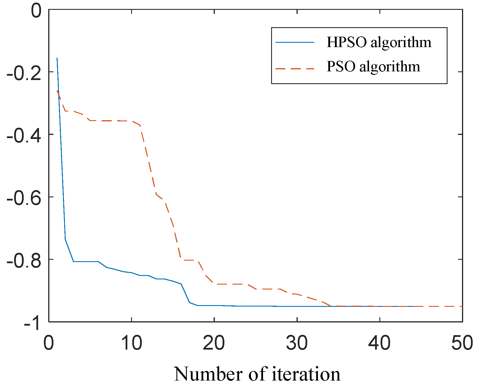
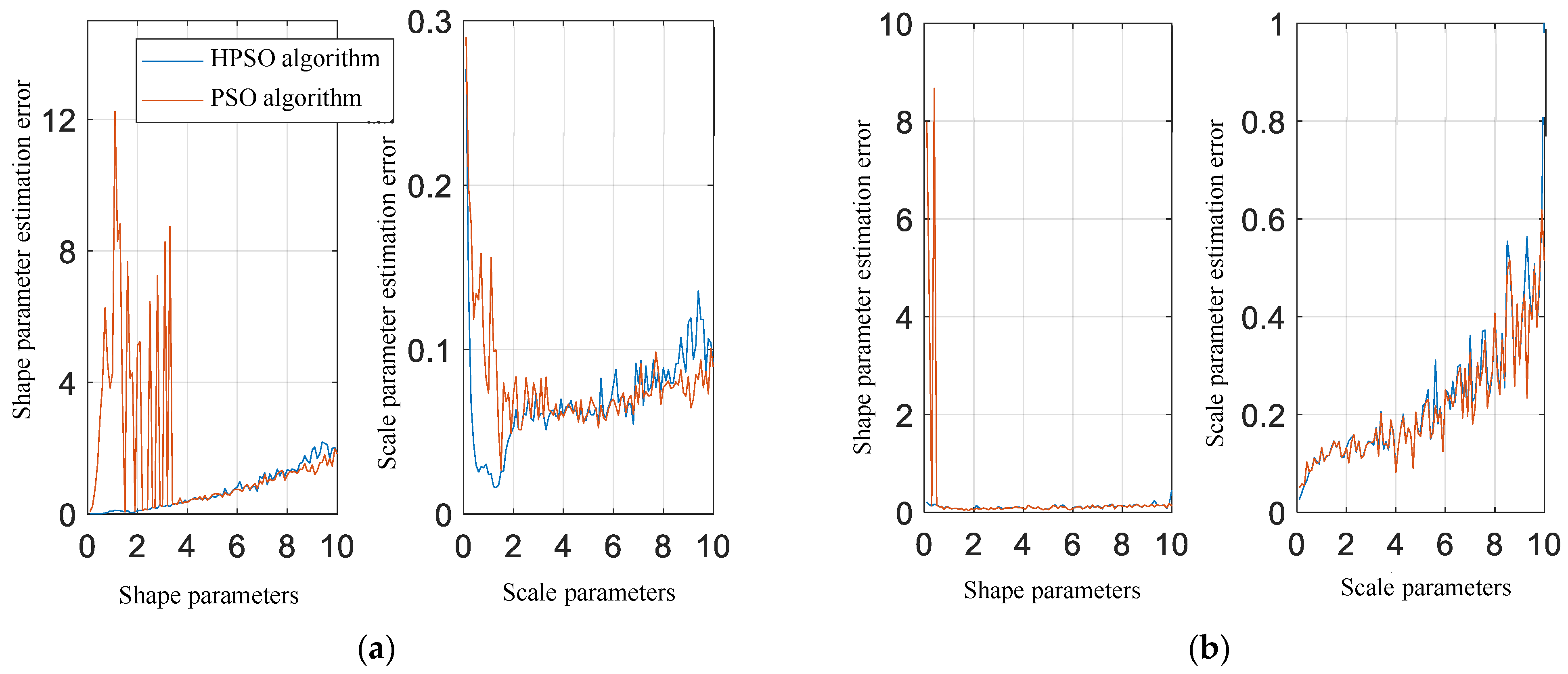
4.3. Performance Analysis of Parameter Estimation with HPSO Algorithm

The parameter settings for the simulation data of the generalized Pareto distribution are as follows: a = 3.5 and b = 0.5, with a total of 5 × 10⁴ samples of noise. We use this simulated data to test the effectiveness of the HPSO algorithm and compare it with the performance of the PSO algorithm. By calculating the fitness values of the simulated data, we can compare the performance differences between these two algorithms in optimizing the objective function. Figure 13 illustrates the iteration process of the HPSO algorithm and the PSO algorithm. From Figure 13, it can be observed that the HPSO algorithm rapidly converges to the global optimum, while the PSO algorithm exhibits slower convergence and may suffer from local convergence. The output parameter estimation results for the optimal positions of both algorithms in the figure are a = 3.2748, b = 0.5729 (HPSO algorithm) and a = 3.2747, b = 0.5729 (PSO algorithm), indicating that the final parameter estimation results are similar for both algorithms. However, the PSO algorithm requires more computation time, with the HPSO algorithm only requiring 18 iterations (while the PSO algorithm requires 35 iterations) to effectively search for the estimated parameters.

To further investigate the performance of the HPSO algorithm in optimizing the objective function for parameter estimation of the generalized Pareto distribution, we fixed either the shape parameter or the scale parameter and varied the other parameter. The PSO algorithm and the HPSO algorithm were employed to search for the global optimal value of the fitness function for parameter estimation of the generalized Pareto distribution. In this way, the corresponding parameter estimation values were obtained. Firstly, we fixed the scale parameter as b = 0.3 and varied the shape parameter of each set of simulated clutter samples from 0.1 to 10 with equal intervals. The number of simulated samples for the generalized Pareto distribution was set as 5 × 10⁴. The experimental results were obtained by averaging the results of 10 repeated experiments. Figure 14a shows the variation curve of the absolute distance between the parameter estimation values obtained by the PSO algorithm and the HPSO algorithm and the actual values.

From Figure 14a, it can be observed that the estimation error of the shape parameter a increases with the increase in the simulated data parameter a, while the estimation error of the scale parameter undergoes a trend of decreasing and then increasing. In addition, the parameter estimation error of the PSO algorithm shows significant variations when the shape parameter a is small, indicating the poor robustness of the parameter estimation using the PSO algorithm.

To fix the shape parameter at a = 2.5, we varied the scale parameter of the clutter samples from 0.1 to 10 with equal intervals, while keeping the length of the simulated data constant. Similarly, the variation curves of the parameter estimation values for both algorithms were plotted (Figure 14b). From Figure 14b, it can be observed that as the scale parameter increases, there is no significant change in the parameter estimation error of the shape parameter a, while the parameter estimation error of the scale parameter b shows an increasing trend. The PSO algorithm still exhibits pronounced oscillations, indicating that the particles in the algorithm are prone to premature convergence, resulting in the population being trapped in local optimal positions. Based on the experimental results mentioned above, it can be concluded that the HPSO algorithm not only achieves higher parameter estimation accuracy compared to the PSO algorithm but also exhibits better stability in parameter estimation. Therefore, in this study, the HPSO algorithm was employed to perform the optimal parameter search task for the fitness function of parameter estimation in the generalized Pareto distribution.

To compare the performance differences of various parameter estimation methods for the generalized Pareto distribution after introducing the HPSO algorithm, this experiment employed the 2nd/4th-moment estimation (2/4th-MoM), 1st-order logarithmic moment estimation (1st-order ZlogZ), and maximum likelihood estimation (MLE) methods. The known parameters were estimated for simulated random sequences of the generalized Pareto distribution, and the results of these three commonly used parameter estimation methods were compared with the HPSO algorithm. The scale parameter b was fixed at 0.5, and the number of clutter samples was 5 × 10⁴. The selection parameter for each set of clutter data varied evenly from 0.1 to 10, with 10 independent repeated experiments conducted. The curves of mean squared deviation (MSD) fitting results for each parameter estimation method were obtained, as shown in Figure 15a. Similarly, by selecting the scale parameter a as 3.5 and varying the selection parameter for each set of clutter data from 0.1 to 10, the variation of the MSD fitting results for each parameter estimation method under different scale parameters was studied (Figure 15b).

Observing Figure 15a, it can be observed that the differences in MSD fitting curves among the parameter estimation methods gradually decrease as the shape parameter increases. In the range where the shape parameter a is less than 2, the HPSO algorithm demonstrates significantly better MSD fitting performance than the 2nd/4th-MoM estimation and the 1st-order ZlogZ estimation method, approaching the fitting performance of the MLE method. Figure 15b shows that as the scale parameter increases, the MSD fitting curves for all four parameter estimation methods gradually decrease. In addition, the MSD test of the MLE method exhibits significant fluctuations in the range of scale parameters from 1 to 2. Moreover, in the region where the scale parameter b is greater than 2, the MSD test values are consistently more than 10⁻² higher than other estimation methods. This indicates that the MLE method’s fitting performance is poorer than the HPSO algorithm, the 2nd/4th-MoM estimation methods, and the 1st-order ZlogZ estimation method.

Based on the results presented in Figure 15, it can be concluded that compared to the other three commonly used parameter estimation methods, the PDF curve of the generalized Pareto distribution approximated by the HPSO algorithm exhibits better robustness and does not suffer from restricted parameter estimation range issues. This algorithm provides a new solution approach for accurately estimating the parameters of the generalized Pareto distribution.

The computational time complexity of the parameter estimation methods is also an indicator for evaluating their performance.

Table 6. Estimate time of different parameter estimation methods.

Parameter Estimation Methods	PSO	HPSO	2nd/4th-MoM	1st-Order ZlogZ	MLE
Running time (s)	3.42 × 10−1	3.22 × 10−1	5.81 × 10−2	2.53 × 10−2	5.56 × 10−1

lists the running times of each parameter estimation method under the same conditions. From Table 6, it can be observed that the 2nd/4th-MoM estimation and the 1st-order ZlogZ estimation method achieve fast parameter estimation processes. The MLE method requires the longest estimation time. Both the PSO algorithm and the HPSO algorithm have the same computational time complexity. Therefore, considering overall performance, the proposed HPSO algorithm demonstrates promising effectiveness in solving the parameter estimation problem for the generalized Pareto distribution.

5. Conclusions

To address the issues in parameter estimation for the generalized Pareto distribution, this study successfully solved the problem of non-closed-form expression using the PSO algorithm and obtained accurate parameter estimates. By expanding the search space of the likelihood function to two dimensions, the stagnation issue in the one-dimensional search was resolved. Fit analysis experiments showed that the positive 0.5th/1st-order fractional moment and positive 0.25th-order logarithmic moment estimation methods performed well in fitting heavy-tailed sea clutter data. To improve the parameter estimation of the PSO algorithm, this research proposed an HPSO algorithm for parameter estimation of the generalized Pareto distribution. Through simulation verification and analysis, the following results were obtained:

• The HPSO algorithm overcame the premature convergence problem of the PSO algorithm and demonstrated better parameter estimation performance.
• The parameters of the HPSO algorithm were optimized, resulting in good performance.
• Through the analysis of parameter estimation variations, it was found that the parameter estimation results of the PSO algorithm were unstable.
• Compared to other methods, the generalized Pareto distribution estimated using the HPSO algorithm exhibited the most stable and optimal fitting results for real data, and it was not influenced by the range of shape parameter values.
• The HPSO algorithm achieved high-precision parameter estimation results while maintaining fast computational speed.

These research findings provide new insights and practical value for parameter estimation of the generalized Pareto distribution. For future research, it is suggested that the influence of different parameter settings in the HPSO algorithm on the optimization process is further investigated and detailed performance analyses using real-world data are conducted.

References

1. Guo, Z.-X.; Bai, X.-H.; Shui, P.-L.; Wang, L.; Su, J. Fast Dual Trifeature-Based Detection of Small Targets in Sea Clutter by Using Median Normalized Doppler Amplitude Spectra. IEEE J. Sel. Top. Appl. Earth Obs. Remote Sens. 2023, 16, 4050–4063. [Google Scholar] [CrossRef]
2. Huang, P.; Yang, H.; Zou, Z.; Xia, X.-G.; Liao, G.; Zhang, Y. Range-Ambiguous Sea Clutter Suppression for Multi-channel Spaceborne Radar Applications Via Alternating APC Processing. IEEE Trans. Aerosp. Electron. Syst. 2023, 1–18. [Google Scholar] [CrossRef]
3. Yin, J.; Unal, C.; Schleiss, M.; Russchenberg, H. Radar Target and Moving Clutter Separation Based on the Low-Rank Matrix Optimization. IEEE Trans. Geosci. Remote Sens. 2018, 56, 4765–4780. [Google Scholar] [CrossRef]
4. Luo, F.; Feng, Y.; Liao, G.; Zhang, L. The Dynamic Sea Clutter Simulation of Shore-Based Radar Based on Stokes Waves. Remote Sens. 2022, 14, 3915. [Google Scholar] [CrossRef]
5. Guidoum, N.; Soltani, F.; Mezache, A. Modeling of High-Resolution Radar Sea Clutter Using Two Approximations of the Weibull Plus Thermal Noise Distribution. Arab. J. Sci. Eng. 2022, 47, 14957–14967. [Google Scholar] [CrossRef]
6. Watts, S.; Rosenberg, L. Challenges in radar sea clutter modelling. IET Radar Sonar Navig. 2022, 16, 1403–1414. [Google Scholar] [CrossRef]
7. Zhao, J.; Jiang, R.; Li, R. Modeling of Non-homogeneous Sea Clutter with Texture Modulated Doppler Spectra. In Proceedings of the 2022 IEEE International Conference on Signal Processing, Communications and Computing (ICSPCC), Xi’an, China, 25–27 October 2022; IEEE: New York, NY, USA, 2022. [Google Scholar]
8. Wang, R.; Li, X.; Zhang, Z.; Ma, H.-G. Modeling and simulation methods of sea clutter based on measured data. Int. J. Model. Simul. Sci. Comput. 2020, 12, 2050068. [Google Scholar] [CrossRef]
9. Amani, M.; Moghimi, A.; Mirmazloumi, S.M.; Ranjgar, B.; Ghorbanian, A.; Ojaghi, S.; Ebrahimy, H.; Naboureh, A.; Nazari, M.E.; Mahdavi, S.; et al. Ocean Remote Sensing Techniques and Applications: A Review (Part I). Water 2022, 14, 3400. [Google Scholar] [CrossRef]
10. El Mashade, M.B. Heterogeneous Performance Assessment of New Approach for Partially-Correlated χ2-Targets Adaptive Detection. Radioelectron. Commun. Syst. 2021, 64, 633–648. [Google Scholar] [CrossRef]
11. Rosenberg, L.; Bocquet, S. The Pareto distribution for high grazing angle sea-clutter. In Proceedings of the 2013 IEEE International Geoscience and Remote Sensing Symposium—IGARSS, Melbourne, VIC, Australia, 21–26 July 2013; IEEE: New York, NY, USA, 2013. [Google Scholar]
12. Mezache, A.; Bentoumi, A.; Sahed, M. Parameter estimation for compound-Gaussian clutter with inverse-Gaussian texture. IET Radar Sonar Navig. 2017, 11, 586–596. [Google Scholar] [CrossRef]
13. Medeiros, D.S.; Garcia, F.D.A.; Machado, R.; Filho, J.C.S.S.; Saotome, O. CA-CFAR Performance in K-Distributed Sea Clutter With Fully Correlated Texture. IEEE Geosci. Remote Sens. Lett. 2023, 20, 1–5. [Google Scholar] [CrossRef]
14. Mahgoun, H.; Taieb, A.; Azmedroub, B.; Souissi, B. Generalized Pareto distribution exploited for ship detection as a model for sea clutter in a Pol-SAR application. In Proceedings of the 2022 7th International Conference on Image and Signal Processing and their Applications (ISPA), Mostaganem, Algeria, 8–9 May 2022; IEEE: New York, NY, USA, 2022. [Google Scholar]
15. Wang, J.; Wang, Z.; He, Z.; Li, J. GLRT-Based Polarimetric Detection in Compound-Gaussian Sea Clutter With Inverse-Gaussian Texture. IEEE Geosci. Remote Sens. Lett. 2022, 19, 1–5. [Google Scholar] [CrossRef]
16. Cao, C.; Zhang, J.; Zhangs, X.; Gao, G.; Zhang, Y.; Meng, J.; Liu, G.; Zhang, Z.; Han, Q.; Jia, Y.; et al. Modeling and Parameter Representation of Sea Clutter Amplitude at Different Grazing Angles. IEEE J. Miniat. Air Space Syst. 2022, 3, 284–293. [Google Scholar] [CrossRef]
17. Fan, Y.; Chen, D.; Tao, M.; Su, J.; Wang, L. Parameter Estimation for Sea Clutter Pareto Distribution Model Based on Variable Interval. Remote Sens. 2022, 14, 2326. [Google Scholar] [CrossRef]
18. Zebiri, K.; Mezache, A. Triple-order statistics-based CFAR detection for heterogeneous Pareto type I background. Signal Image Video Process. 2023, 17, 1105–1111. [Google Scholar] [CrossRef]
19. Hu, C.; Luo, F.; Zhang, L.; Fan, Y.; Chen, S. Widening valid estimation range of multilook Pareto shape parameter with closed-form estimators. Electron. Lett. 2016, 52, 1486–1488. [Google Scholar] [CrossRef]
20. Shui, P.L.; Zou, P.J.; Feng, T. Outlier-robust truncated maximum likelihood parameter estimators of generalized Pareto distributions. Digit. Signal Process. 2022, 127, 103527. [Google Scholar] [CrossRef]
21. Tian, C.; Shui, P.-L. Outlier-Robust Truncated Maximum Likelihood Parameter Estimation of Compound-Gaussian Clutter with Inverse Gaussian Texture. Remote Sens. 2022, 14, 4004. [Google Scholar] [CrossRef]
22. Shui, P.L.; Tian, C.; Feng, T. Outlier-robust Tri-percentile Parameter Estimation Method of Compound-Gaussian Clutter with Inverse Gaussian Textures. J. Electron. Inf. Technol. 2023, 45, 542–549. [Google Scholar] [CrossRef]
23. YU, H.; Shui, P.L.; Shi, S.N.; Yang, C.J. Combined Bipercentile Parameter Estimation of Generalized Pareto Distributed Sea Clutter Model. J. Electron. Inf. Technol. 2019, 41, 2836–2843. [Google Scholar] [CrossRef]
24. Xue, J.; Xu, S.; Liu, J.; SHUI, P. Model for Non-Gaussian Sea Clutter Amplitudes Using Generalized Inverse Gaussian Texture. IEEE Geosci. Remote Sens. Lett. 2019, 16, 892–896. [Google Scholar] [CrossRef]
25. Xia, X.-Y.; Shui, P.-L.; Zhang, Y.-S.; Li, X.; Xu, X.-Y. An Empirical Model of Shape Parameter of Sea Clutter Based on X-Band Island-Based Radar Database. IEEE Geosci. Remote Sens. Lett. 2023, 20, 1–5. [Google Scholar] [CrossRef]
26. Liang, X.; Yu, H.; Zou, P.-J.; Shui, P.-L.; Su, H.-T. Multiscan Recursive Bayesian Parameter Estimation of Large-Scene Spatial-Temporally Varying Generalized Pareto Distribution Model of Sea Clutter. IEEE Trans. Geosci. Remote Sens. 2022, 60, 1–16. [Google Scholar] [CrossRef]
27. Tang, J.; Liu, G.; Pan, Q. A Review on Representative Swarm Intelligence Algorithms for Solving Optimization Problems: Applications and Trends. IEEE/CAA J. Autom. Sin. 2021, 8, 1627–1643. [Google Scholar] [CrossRef]
28. Wei, X.; Huang, H. A Survey on Several New Popular Swarm Intelligence Optimization Algorithms; Research Square Platform LLC: Durham, NC, USA, 2023. [Google Scholar]
29. Hong, S.-H.; Kim, J.; Jung, H.-S. Special Issue on Selected Papers from “International Symposium on Remote Sensing 2021”. Remote Sens. 2023, 15, 2993. [Google Scholar] [CrossRef]
30. Shui, P.-L.; Yu, H.; Shi, L.-X.; Yang, C.-J. Explicit bipercentile parameter estimation of compound-Gaussian clutter with inverse gamma distributed texture. IET Radar Sonar Navig. 2018, 12, 202–208. [Google Scholar] [CrossRef]
31. Sergievskaya, I.A.; Ermakov, S.A.; Ermoshkin, A.V.; Kapustin, I.A.; Shomina, O.V.; Kupaev, A.V. The Role of Micro Breaking of Small-Scale Wind Waves in Radar Backscattering from Sea Surface. Remote Sens. 2020, 12, 4159. [Google Scholar] [CrossRef]
32. Hu, C.; Luo, F.; Zhang, L.R.; Fan, Y.F.; Chen, S.L. Widening Efficacious Parameter Estimation Range of Multi-look Pareto Distribution. J. Electron. Inf. Technol. 2017, 39, 412–416. [Google Scholar] [CrossRef]
33. Kennedy, J.; Eberhart, R. Particle swarm optimization. In Proceedings of the ICNN’95—International Conference on Neural Networks, Perth, WA, Australia, 27 November–1 December 1995; IEEE: New York, NY, USA, 2002. [Google Scholar]
34. Wu, J.; Hu, J.; Yang, Y. Optimized Design of Large-Body Structure of Pile Driver Based on Particle Swarm Optimization Improved BP Neural Network. Appl. Sci. 2023, 13, 7200. [Google Scholar] [CrossRef]
35. Xu, Z.; Xia, D.; Yong, N.; Wang, J.; Lin, J.; Wang, F.; Xu, S.; Ge, D. Hybrid Particle Swarm Optimization for High-Dimensional Latin Hypercube Design Problem. Appl. Sci. 2023, 13, 7066. [Google Scholar] [CrossRef]
36. Chandrashekar, C.; Krishnadoss, P.; Kedalu Poornachary, V.; Ananthakrishnan, B.; Rangasamy, K. HWACOA Scheduler: Hybrid Weighted Ant Colony Optimization Algorithm for Task Scheduling in Cloud Computing. Appl. Sci. 2023, 13, 3433. [Google Scholar] [CrossRef]
37. Wang, D.; Meng, L. Performance Analysis and Parameter Selection of PSO Algorithms. Acta Autom. Sin. 2016, 42, 1552–1561. [Google Scholar]
38. Xu, S.; Wang, L.; Shui, P.; Li, X.; Zhang, J. Iterative maximum likelihood and zFlogz estimation of parameters of compound-Gaussian clutter with inverse gamma texture. In Proceedings of the 2018 IEEE International Conference on Signal Processing, Communications and Computing (ICSPCC), Qingdao, China, 14–16 September 2018; IEEE: New York, NY, USA, 2018. [Google Scholar]
39. Xu, S.; Ru, H.; Li, D.; Shui, P.; Xue, J. Marine Radar Small Target Classification Based on Block-Whitened Time–Frequency Spectrogram and Pre-Trained CNN. IEEE Trans. Geosci. Remote Sens. 2023, 61, 1–11. [Google Scholar] [CrossRef]
40. Li, D.; Zhao, Z.; Zhao, Y. Analysis of Experimental Data of IPIX Radar. In Proceedings of the 2018 IEEE International Conference on Computational Electromagnetics (ICCEM), Chengdu, China, 26–28 March 2018; IEEE: New York, NY, USA, 2018. [Google Scholar]
41. Ding, H.; Liu, N.B.; Dong, Y.L.; Chen, X.L.; Guan, J. Overview and Prospects of Radar Sea Clutter Measurement Experiments. J. Radars 2019, 8, 281–302. [Google Scholar] [CrossRef]
42. Liu, N.B.; Ding, H.; Huang, Y.; Dong, Y.L.; Wang, G.Q.; Dong, K. Annual Progress of the Sea-detecting X-band Radar and Data Acquisition Program. J. Radars 2021, 10, 173–182. [Google Scholar] [CrossRef]
43. Fan, Y.; Tao, M.; Su, J.; Wang, L. Analysis of goodness-of-fit method based on local property of statistical model for airborne sea clutter data. Digit. Signal Process. 2020, 99, 102653. [Google Scholar] [CrossRef]
44. Huang, P.; Zou, Z.; Xia, X.-G.; Liu, X.; Liao, G. A Statistical Model Based on Modified Generalized-K Distribution for Sea Clutter. IEEE Geosci. Remote Sens. Lett. 2022, 19, 1–5. [Google Scholar] [CrossRef]
Figure 1. Generalized Pareto distribution amplitude PDF curve.
Applsci 13 09115 g001
Figure 2. HPSO algorithm flowchart.
Applsci 13 09115 g002
Figure 3. Statistical histogram of simulation data.
Applsci 13 09115 g003
Figure 4. The curve of the fitness function.
Applsci 13 09115 g004
Figure 5. Particle trajectory of the first fitness function.
Applsci 13 09115 g005
Figure 6. Particle trajectory of the second fitness function.
Applsci 13 09115 g006
Figure 7. Particle trajectory of the third fitness function.
Applsci 13 09115 g007
Figure 8. Comparison of spatial search in different dimensions of the maximum likelihood function.
Applsci 13 09115 g008
Figure 9. Parameter estimation performance as a function of shape parameters. (a,b) indicate the trends of RRMSE metrics with shape parameters for scale and shape parameters, respectively.
Applsci 13 09115 g009
Figure 10. Fitting results of IPIX radar measured data.
Applsci 13 09115 g010
Figure 11. Fitting effect of generalized Pareto distribution.
Applsci 13 09115 g011
Figure 12. The fitting effect chart of the SMSD test.
Applsci 13 09115 g012
Figure 13. Comparison of two different algorithms’ iterative processes.
Applsci 13 09115 g013
Figure 14. Parameter estimation error curves of two different algorithms. (a,b) denote the estimation errors of the corresponding parameters when the shape and scale parameters are varied at equal intervals, respectively.
Applsci 13 09115 g014
Figure 15. Parameter estimation error curves of two different algorithms. (a,b) denote the fitting errors when the shape and scale parameters are varied at equal intervals, respectively.
Applsci 13 09115 g015