Featured Application
Prediction of orthopedic implant stability, particularly pedicle screws, as an index comparable to insertion torque.
Abstract
To prevent pedicle screw implant failure, a diagnostic technique that allows surgeons to evaluate implant stability easily, quickly, and quantitatively in clinical orthopedic situations is required. This study aimed to predict the insertion torque equivalent to laboratory-level evaluation accuracy. This serves as an index of the implant stability of pedicle screws placed in cadaveric bone, which relies on laser resonance frequency analyses (L-RFA) when irradiating with two types of lasers. The machine learning analysis was optimized using a dataset with artificial bone as teaching data. In this analysis, many explanatory variables extracted from the laser-induced vibration spectra obtained during an analysis/RFA evaluation were predicted by selecting important variables using the least absolute shrinkage and selection operator and performing a non-linear approximation using support vector regression. It was found that combining both artificial and cadaveric bone data with the bone densities as teaching data dramatically improved the determination coefficient from R2 = −0.144 to R2 = 0.858 as the prediction accuracy and reduced the influence of differences between artificial and cadaveric bones. This technology will contribute to the development of preventive diagnostic technologies that can be used during surgery, which is necessary in order to further advance treatment technologies.
1. Introduction
With the advent of an aging society, the use of orthopedic implants with pedicle screws in the field of orthopedic surgery has increased [1,2]. Orthopedic surgery for pedicle screw placement aims to achieve spinal stabilization during spinal procedures. After visualizing the spinal bone, a pilot hole is created to guide the pedicle screw implant, which can be expanded by tapping. Thereafter, a pedicle screw is inserted into the tapping hole. The screw is preselected based on its diameter and length and positioned to ensure bone fixation. Once the screw is properly positioned, it is secured using a fixation device, such as a plate, rod, or nut, which stabilizes the spine. However, this procedure is performed based on the hand feeling and experience of the primary surgeon. Implant failure has become problematic, with reported incident and revision rates of 12% [3] and 40% [4], respectively. To overcome this problem, the initial implant stability is evaluated as an index [5,6]. The pullout force [7] and insertion torque tests [5,8] were used to evaluate the initial implant stability as an index. Pullout force tests are destructive laboratory tests that cannot be used in clinical situations. Although the insertion torque can be measured during surgery, it is a one-time, non-repeatable measurement, and is influenced by factors attributable to each surgeon, such as the implantation speed and applied force. To address this problem, laser resonance frequency analysis (L-RFA) was used to measure the implant stability of pedicle screws [9,10] and acetabular cups [11]. The L-RFA with laser technology was developed to replace hammering tests used for structural infrastructure [12]. Vibrations induced by active excitation are used as a basic principle of hammering inspection, and the induced vibration is detected by the ear, where the condition is determined by the sound information. For tunnel inspections, a hammering test is used to survey nonvisible internal defects in concrete walls and detect loose bolts. The principle of L-RFA is to replace active excitation with laser irradiation to induce vibrations via laser ablation or laser-induced photoacoustic–elastic waves (LIPTEW) [13]. By measuring and analyzing the LIPTEW with a laser Doppler vibrometer, the L-RFA realizes high-speed, remote, and quantitative evaluations.
Implant stability diagnosis using RFA is widely used in the dental field with magnetic excitation [14]. This method is widely used because the oral cavity can be opened widely and still allows for fine magnet installation [15]. However, orthopedic implants are not used because of the low strength of magnetic excitation and the difficulty of intraoperative placement of fine magnets [16]. Because of the difficulty of excitation by magnets, the use of mechanical vibrators has been considered, but no clear correlation has been obtained [17,18,19]. However, the L-RFA reported in 2019 shows the potential for use in the orthopedic field [11].
The natural vibrations in the audible frequency range of the experimental sample were measured using L-RFA. The natural vibration frequency obtained using L-RFA indicates implant stability determined by the interaction between the implant surface and the bone texture on which it is placed, similar to conventional pullout force and insertion torque tests. Therefore, the implant stability estimated in the L-RFA is predicted from the correlation expressed in terms of the natural vibration frequency and mechanical strength to be evaluated in the L-RFA [9,10,11]. However, the correlation between the natural vibration frequencies measured by the L-RFA and the insertion torque experiences reduced prediction accuracy, with a coefficient of determination of R2 = 0.867 for artificial bone using a logarithmic approximation, and R2 = 0.513 for cadaveric bone [10]. In addition to the difference between artificial and cadaveric bones, another issue with L-RFA is that the natural vibration frequency varies depending on the mechanical properties and shape of the evaluation sample, which can easily lead to errors. In recent years, highly accurate L-RFA has been performed using machine learning-based analyses that utilize multiple explanatory variables instead of one index of natural vibration frequency. It was reported that for a polyaxial screw with a movable neck, whose natural frequency is unstable owing to changes in the sample shape, machine learning-based analysis provides the same accuracy for implant stability as that of a monoaxial screw with a fixed shape [20].
Machine learning-based analysis techniques require large amounts of high-quality teaching data. Because L-RFA is based on the evaluation principle of measuring the natural vibration of orthopedic implants, teaching data must be prepared for each implant. However, accumulating teaching data in the clinical field is difficult because of their mechanical strength, which can be obtained through destructive testing. In addition, it is challenging to conduct non-clinical tests using cadaveric bone because the variation in donors is biased and a limited number of tests can be conducted. Therefore, it is desirable to utilize data obtained from artificial bones as teaching data, similar to previous studies [9,10,11]. Although differences in the structure and composition of artificial and cadaveric bones are expected to affect the accuracy of implant stability estimation, a combined analysis of these types of bone data has not been considered in previous studies [10]. In addition, although the L-RFA in previous studies was determined via the relative relationship between the implant and the bone; it did not utilize bone information, and only the natural vibration frequency of the implant was examined. Therefore, by introducing density, which provides information on the foundation, higher accuracy in estimating implant stability is anticipated.
In this study, a machine learning analysis method combining L-RFA data of artificial bone, as well as the bone-density data of cadaveric bone obtained using micro-computed tomography, was used to verify the prediction accuracy of stability for a pedicle screw implant installed in cadaveric bone using L-RFA. Computed tomography (CT) is a widely used imaging modality in the field of medicine, providing detailed cross-sectional images of the human body. Since its introduction in the 1970s, CT has revolutionized diagnostic medicine by offering a non-invasive and rapid imaging technique that allows for the detection, characterization, and monitoring of various diseases and conditions. Micro-CT is a specialized imaging technique designed for the high-resolution imaging of small specimens or samples. It employs a micro-focus X-ray source and detector to generate detailed three-dimensional images of structures with sub-millimeter or even sub-micrometer spatial resolutions. Micro-CT is particularly useful in research and preclinical studies as it provides valuable insights into the microscopic structures of tissues, bones, biomaterials, and small animal models. By augmenting the L-RFA data evaluated using artificial bone and introducing bone-density data, which is a clinical parameter, an analytical method that is comparable to the estimation accuracy reported for ideal artificial bone data was developed. The results of this study connect the results of laboratory-level evaluation using artificial bone with those of clinical-level evaluation obtained from biological bone. This study will contribute to the development of diagnostic techniques for implant stability.
2. Methods and Materials
The proposed analysis scheme based on machine learning uses the L-RFA dataset reported in a previous study [10]. The machine learning-based analysis method proposed in this study is based on improving generalizability by introducing bone density, a clinical parameter, into a previously reported scheme [20]. First, the detail of dataset [10] and the conventional machine learning-based analysis method [20] are presented. After that, bone-density analysis using CT is described to obtain the key-data for the analysis method.
2.1. Detail of Dataset and Analysis Method
2.1.1. Analyzed Materials
Five types of solid polyurethane foams were prepared as artificial bones, which represented the vertebrae used for the measurement data. Each type represented a different density and was cut to a size of 60 × 40 × 60 mm, with a screw placed at the center of the material on a 60 × 40 mm surface, after which 27 measurements were conducted. Unfrozen cadaveric bone was used after receiving approval from the Ethical Review Committee of Keio University School of Medicine (approval number 20150385), and written informed consent was obtained from each donor in accordance with the guidelines. Nine sections of the two human lumbar spines (L1–L5; 10 vertebrae) were used in this study, excluding one vertebra that was damaged during preparation. Two pedicle screws were placed per vertebra for a total of 17 conditions measured, excluding one missed placement.
The screws to be placed in the artificial and cadaveric bones were monoaxial titanium alloy (Ti-6Al-4V, ASTM F136) screws (catalog no. CMS05135, Kyocera, Corp., Kyoto, Japan). The pedicle screw was inserted at a length of 40 mm, with 5 mm remaining at the base of the screw. Paik et al. reported that when a screw head is inserted until it contacts the bone, it causes bone fracture and reduces the fixation force [21]. Therefore, the technique used in this study did not allow the screw heads to contact the specimen in a manner similar to that used in clinical practice. All screws were inserted at the same depth (40 mm) using a depth gauge.
The torque at the time of insertion was measured using a digital torque gauge (HTGA-5N, IMADA Co., Ltd., Aichi, Japan) to evaluate the insertion torque (peak torque) at a 40 mm insertion. This method of measuring insertion torque is identical to that of the conventional method [16,22,23,24].
2.1.2. L-RFA Evaluation
In the L-RFA, two lasers are used: an impact laser to induce vibration on the screw and a measurement laser to evaluate the induced vibration. An Nd: YLF laser was used as the impact laser. A laser Doppler vibrometer (PDV-100, Polytec GmbH, Baden-Württemberg, Germany) was used as a measurement laser. Both lasers were irradiated at the neck of the screw, and the measurement laser was irradiated. The vibration time-series data were synchronized to the Q-switched signal of the laser pulse irradiation, and the data (1.6 s) for 16 pulse irradiations were stored. The obtained signals were divided into 16 pulses of laser-induced vibration for each pulse irradiation, and the laser-induced vibrational frequency spectrum was obtained using a fast Fourier transform with a rectangular window function by trimming the data for 4.5 ms after the impact laser pulse irradiated. The purpose of the data trim was to obtain a clear frequency peak arising from the natural vibrations in the audible region. This was achieved by eliminating the noise associated with the burst sound caused by plasma formation arising from laser ablation.
2.1.3. Machine Learning-Based Analysis Scheme
In previous studies on the L-RFA evaluation of orthopedic implants, a correlation evaluation between implant stability and the strongest vibration frequency obtained by L-RFA was performed. From this correlation evaluation, it was found that the vibration frequency obtained via L-RFA increased as implant stability increased [9,10,11]. However, using only this correlation evaluation has been shown to reduce the estimation accuracy of cadaveric bones [10]. Multivariate analysis is effective because there are many modes of natural vibration, from basic to a higher order, each of which contains information on implant stability. In general, deep learning requires a large amount of high-quality training data. However, the amount of data managed in this study was limited because of the data requirements for each implant type and the repeatability limitations associated with clinical practices. Therefore, it is necessary to consider a machine learning scheme that can achieve high accuracy even with a small amount of training data. To date, methods were proposed using machine learning, the least absolute shrinkage and selection operator (LASSO), and support vector regression (SVR) for multivariate analyses [20].
Our proposed machine learning-based analysis process consists of two main schemes, the first of which introduces LASSO [25,26] as an explanatory variable selection process. In the conventional method, the only explanatory variable evaluated for correlation with the embedded torque is the peak vibration frequency. However, many explanatory variables, such as the intensity and dispersion, are stored in the vibration frequency spectrum and spread over the entire measurement frequency range. Therefore, it was possible to divide the frequency range in which the analysis was performed and extract each explanatory variable for each range. Eight variables (peak frequency, peak intensity, frequency center of gravity, intensity center of gravity, average intensity, variance, kurtosis, and skewness) were extracted for eight frequency ranges (30–150 Hz, 150–500 Hz, 500–1000 Hz, 1000–5000 Hz, 5000–10,000 Hz, 10,000–15,000 Hz, 15,000–20,000 Hz, and 30–20,000 Hz). In this study, explanatory variables of total 64 explanatory variables were prepared from the L-RFA dataset reported in a previous study [10]. As a specific procedure, regularization was performed to smooth the orders of the explanatory and objective variables. The lasso was performed 2000 times with multiple regularization strengths, and 40 data points were extracted to determine the regularization strength at the best decision coefficient. The important explanatory variables were ranked by the regularization strength determined by sorting the data in the order of the number of times they were selected.
The second scheme uses SVR to perform non-linear regression, which is an adaptation of the support vector machine (SVM) [27,28], a pattern recognition method for regression that can be adapted to non-linear problems by incorporating a kernel function. In this study, a radial basis function (RBF) kernel, which is computationally fast and accurate, was used. Here, a promising regression technique in addition to SVR is multiple regression analysis. Multiple regression analysis provides an intuitive interpretation of the relationship between multiple explanatory and objective variables, indicating the magnitude and direction of the effect of the coefficient of each explanatory variable on the objective variable. However, multiple regression analysis assumes that a linear relationship exists between explanatory and objective variables. The predictive performance of the model may be affected for data with non-linear relationships. In addition, in multiple regression analysis, multicollinearity problems can occur when high correlations exist among the explanatory variables. This can make it difficult to accurately assess the impact of explanatory variables. Furthermore, multiple regression analysis assumes that the explanatory and objective variables follow a normal distribution. However, for non-normal data, this can affect the interpretation of results and predictive performance. Therefore, SVR was used in this study.
The hyperparameters required to train the SVR are determined by cross validation on a total of 15,750 pattern presented by grid search, insensitivity coefficient ε in the range 2−20 to 29, regularization coefficient C in the range 2−10 to 210, and RBF kernel function γ in the range 2−15 to 29. The combination with the highest coefficient of determination was used as the adequate hyperparameter. As with LASSO, standardization was used to smooth the orders of the explanatory and objective variables when performing SVR, and the explanatory variables ranked by importance in LASSO were changed to search for regression results with the highest coefficient of determination.
2.2. Bone-Density Observation by Micro-CT Analysis
The bone densities of the artificial bones were those specified for the product, which are 5, 10, 12, 20, and 30 pcf, respectively. On the other hand, the bone density of the cadaveric bone was determined using micro-CT. Figure 1 shows an example of a micro-CT image of a cadaveric bone. Bone-density estimation using micro-CT image data extracted from digital imaging and communications in medicine (DICOM) data consists of preprocessing for image noise removal, bone region extraction based on thresholding and morphology processing, and a comparative analysis of the bone region volume and high-intensity region volume inside the bone region. DICOM, which was initially developed in the 1980s, provides a unified format for storing, transmitting, and sharing medical images and associated patient information across different healthcare systems and devices. DICOM has become the de facto standard for medical imaging because of its comprehensive specifications and support for a wide range of imaging modalities, including X-rays, CT, magnetic resonance imaging (MRI), ultrasound, and nuclear medicine. Preprocessing uses a mid-value filtering process with a spherical kernel of radius one voxel. The bone region extraction procedure consisted of binarization at luminance values of 4000 or higher, extraction of the connected component of the largest volume, and filling of the extracted region. The connected component of the maximum volume was obtained based on the results of the 3D labeling process for the area obtained by binarization (3D labeled image). Bone regions were extracted by closing and hole-filling processes to obtain the maximum volume component. First, a 3D morphological closing process using a spherical kernel with a radius of 4.5 voxels was applied to the extracted maximum volume component region. Next, 2D hole-filling of the region was performed on each axial slice. The same 3D morphological closure process was repeated to determine the final bone region. Finally, the volume of the extracted bone region and the high-intensity region within the bone region with a luminance value of 4000 or higher were measured, and the volume ratio of the high-intensity region to the bone region was calculated. Each parameter employed in the above process was experimentally optimized.
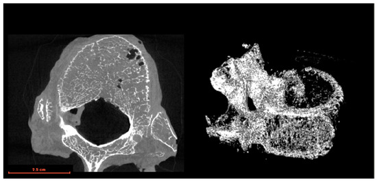
Figure 1.
Example of a micro-CT image of cadaveric bone.
The percentage of luminance values greater than 4000 obtained from micro-CT scans ranged from 0.486 to 0.664, with a mean value of 0.537 and a standard deviation of 0.0513. The absolute value of the bone density was determined from the proportions obtained from phantom measurements [25] in previous studies. In this study, an approximation was made by fitting a high coefficient of determination of the peak torque and bone density at the time of implantation obtained from the simulated bones, as shown by the circular plot in Figure 2. The percentage of the peak torque evaluation results for each cadaveric bone with a luminance value of 4000 or higher was used as the bone density to determine the bone density shown in the square plots to minimize the squared error with fitting. As a result, the bone density of the cadaveric bones was estimated to be equivalent to 7.73 pcf to 10.5 pcf. The bone density was included into the dataset as a clinical parameter, yielding a total of 65 variables and utilizing a dataset standardized by each explanatory variable.
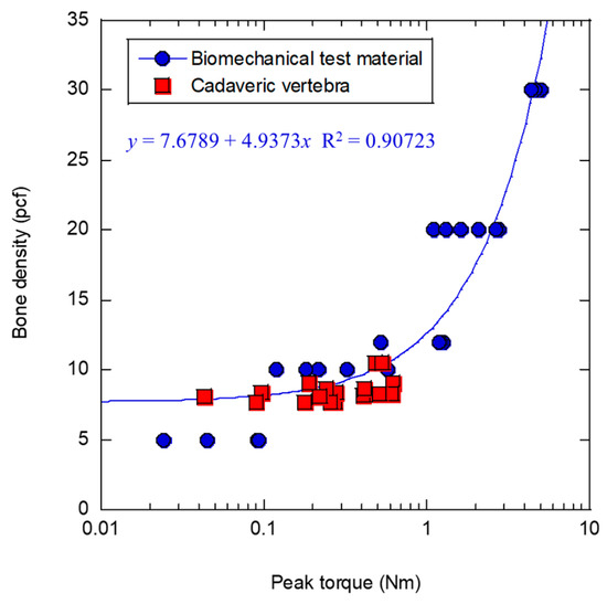
Figure 2.
Relationship between peak torque and bone density.
For bone-density information in this study, only the value averaged over the entire bone was used as a feature. In the future, accuracy may be improved by introducing information on the fine reticular structure and structure of the cortical and trabecular bones. However, because the information to be used in clinical practice will be obtained from multislice CT, it is expected to be more convenient to use the overall average value, as in the present study. It is also possible to introduce values measured using dual-energy X-ray absorptiometry (DEXA).
3. Result and Discussion
The proposed analysis scheme is based on machine learning and uses the L-RFA dataset reported in a previous study [10]. When assuming clinical derivation, it is desirable to use the evaluation results of the L-RFA measured at the laboratory level to predict the implant stability of screws in cadaveric bones. Therefore, in this study, the possibility of analyzing the stability of screws installed in cadaveric bones was verified using the results of the L-RFA evaluations of artificial bones. The analysis method was examined, and bone-density data were introduced to improve prediction accuracy.
3.1. Performance of Teaching Data with Only Biomechanics Materials
Using the machine learning scheme described in Section 2.1.3, the L-RFA measurement dataset of the artificial bone was used as teaching data to predict the peak torque from the L-RFA data of the cadaver bone and was compared with the measured peak torque. Three cases of validation were performed using only artificial bone as teaching data: the first was simple, with no data processing; the second was limited to training data below 1.04 Nm in the low peak torque range where cadaver bone data existed; and the third was data augmentation of the training data by linear interpolation. Table 1 shows the results obtained using the three analysis schemes, including the number of explanatory variables obtained using LASSO, coefficient of determination, and mean squared error (MSE) methods at the time of the highest SVR performance.

Table 1.
Experimental results obtained using the three analysis schemes with only the artificial bone dataset.
3.1.1. Simple Data Set
The first analysis method, the L-RFA dataset of artificial bones, was analyzed as teaching data without additional processing. The predicted results for cadaver bones are shown in Figure 3. Figure 3a shows the correlation between the measured and predicted values, with the solid line indicating the ideal result and the measured and predicted values match. Figure 3b is a Bland–Altman plot, which is a method used to evaluate the agreement between two measurement methods. In this study, the agreement between the measured and predicted values was evaluated. The horizontal axis represents the measured and predicted mean values for each data point, and the vertical axis represents the difference between them. The dotted line in the figure represents the limits of agreement, which is the statistical 95% confidence interval obtained by subtracting the standard deviation multiplied by 1.96 from the mean of the difference between the two datasets, which can be interpreted as equivalent if found within this dotted line. As shown in Figure 3a, the coefficient of determination R2 = −0.144 indicates no relationship. The four explanatory variables used were peak frequency (1000–5000 Hz), peak frequency (30–20,000 Hz), variance (500–1000 Hz), and skewness (500–1000 Hz). The Bland–Altman plot in Figure 3b shows that there was a weak fixed error of up to 0.4 on the horizontal axis, followed by a proportional error. This result indicates that the influence of random errors is small and that systematic errors due to fixed and proportional errors lead to lower prediction accuracy. Therefore, by correcting for this uniform error in advance, it is possible to predict implant stability in cadaveric bone using L-RFA data of artificial bones obtained at the laboratory level. However, it is preferable to avoid adding further data processing to correct errors because of concerns regarding generalizability and prediction accuracy degradation. Therefore, the improvement in the prediction accuracy should be investigated by devising teaching data in advance.
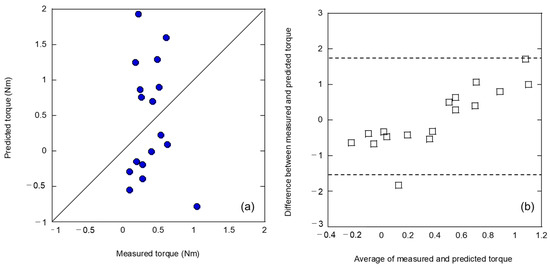
Figure 3.
Analysis results of (a) relationship between measured and predicted insertion torques and (b) Bland–Altman plot by teaching the dataset without additional processing.
3.1.2. Data Augmentation by Linear Interpolation
In general, machine learning is expected to improve the accuracy of analysis as the amount of training data increases. Therefore, an attempt was made to augment the training data using linear interpolation. In this linear interpolation, 30 data points were assumed with two peak torques and intermediate values of explanatory variables in the middle of each data point for the 31 training data points. Figure 4 shows the results of the analysis of the 31 teaching data points and 30 linearly interpolated data points for 61 teaching data points. The correlations in Figure 4a exhibit the same trends as those in Figure 3a. The explanatory variables used in this case were the same as before data augmentation: peak frequency (1000–5000 Hz) and frequency center of gravity (150–500 Hz). However, both the coefficient of determination and MSE resulted in inferior performance. For the Bland–Altman plot shown in Figure 4b, a clear systematic error with fixed and proportional errors was identified, as shown in Figure 3b. This clearly indicates that data augmentation using simple linear interpolation was ineffective. This suggests that the analytical performance shown in Figure 3 is not due to an insufficient amount of teacher data, but rather because of the difference in the potential foundation between the artificial and cadaveric bones.
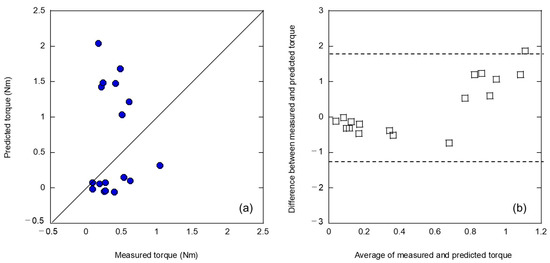
Figure 4.
Analysis results of (a) relationship between measured and predicted insertion torques and (b) Bland–Altman plot by augmentation of the teaching data by linear interpolation.
3.1.3. Range Limitation of Torque
In machine learning, the teaching data must be close to the range of the analyzed data for prediction as well as the number of such data. Therefore, because the peak torque of the artificial bone was up to approximately 5 Nm, whereas the peak torque of the cadaveric bone data was up to approximately 1 Nm, the artificial bone data were analyzed using the teaching data by reducing the number of data to 18, limiting the peak torque range to the same as that of the cadaveric bone. The results of this analysis are shown in Figure 5. As shown in Figure 5a, different correlations were obtained from those in Figure 3a and Figure 4a, although the accuracy of the analysis was worse because of the data range restrictions. The two variables used were frequency weighted (5000–10,000 Hz) and frequency weighted (1000–5000 Hz). The Bland–Altman plot shown in Figure 5b indicates that while systematic errors disappeared because of the limited data range, random errors appeared. This can be attributed to the small amount of available teaching data.
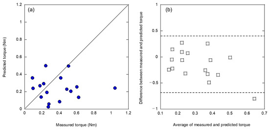
Figure 5.
Analysis result of (a) relationship between measured and predicted insertion torques and (b) Bland–Altman plot by limiting the peak torque range to the same as that of the cadaveric bone dataset.
The method of analyzing L-RFA data using an artificial bone as a teaching dataset to predict the peak torque by validating L-RFA data using cadaveric bone was found to have a clear emergence of systematic errors. However, there is a concern that an a priori evaluation and correction of the error will increase the data analysis process and reduce its generalizability, convenience, and accuracy. Therefore, it is necessary to improve accuracy by applying further innovations.
3.2. Improvement of Prediction Performance by Data Augmentation
To predict the peak frequency—an indicator of implant stability in cadaveric bone—using machine learning-based analysis, the accuracy was improved by adding data other than those obtained by L-RFA using artificial bone to the teaching data. As shown in Figure 3 and Figure 4, it is possible that the difference in foundation between the artificial and cadaveric bones potentially influenced the L-RFA results. Using this experimental finding as a guide, the artificial bone-teaching dataset was augmented using a small amount of cadaveric bone data. Furthermore, bone density was introduced as a parameter obtained in clinical practice, and an explanatory variable was obtained outside the L-RFA assessment. As a validation method, a three-fold cross validation was performed by combining 31 datasets from artificial bones with L-RFA evaluation and 17 datasets from cadaveric bones. Each fold was created equally, such that the peak torque was unbiased, and the percentage of data from the donated bones was approximately 35%. Table 2 summarizes the results of this three-fold validation of the machine learning performance with and without the introduction of bone density.
Table 2.
Experimental results of the three-fold validation of machine learning performance with and without the introduction of bone density.
3.2.1. Without Bone Density
Figure 6 shows the results of a three-fold cross validation using a mixed dataset of artificial and cadaveric bones without introducing bone density. As shown in Figure 6a, the regression performance was dramatically improved compared to the dataset obtained in the previous L-RFA evaluation using artificial bone, as shown in Figure 3, Figure 4 and Figure 5. The average coefficient of determination for the three-fold cross validation was R2 = 0.697, yielding an MSE of 0.208. The four explanatory variables utilized were peak frequency (1000–5000 Hz), skewness (500–1000 Hz), frequency center of gravity (1000–5000 Hz), and variance (500–1000 Hz). The variables selected in this LASSO were a combination of the explanatory variables used in the two types of analyses: the simulated bone data-only teacher dataset shown in Figure 3; and the teaching dataset restricted to the peak frequency range of the cadaveric bones shown in Figure 5. This suggests that explanatory variables that are more representative of cadaveric bone validation data may have been utilized with the teaching data from the artificial bone dataset as a substrate. As shown in Figure 6b, the Bland–Altman plot describes the prediction results for the artificial and cadaveric bones separately, and the cadaveric bone data showed a rightward proportional error, indicating the need for a correction for the prior error, as shown in Figure 4b.
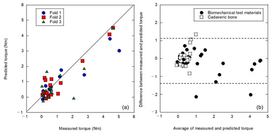
Figure 6.
Analysis results of a three-fold cross validation using a mixed dataset of artificial and cadaveric bones without bone density: (a) relationship between measured and predicted insertion torques; (b) Bland–Altman plot.
3.2.2. With Bone Density
Previous analyses have shown that differences between potential artificial and cadaveric bones can affect the analysis results. Therefore, the analysis was conducted by introducing the bone density of the clinical data, which is foundational information, as a feature of the teaching data. Each fold was the same as that in the analysis without bone density, as shown in Figure 6. The evaluation results are shown in Figure 7. The highest prediction accuracy was obtained in this analysis, as shown in Figure 7a. A three-fold average coefficient of determination R2 = 0.858 and MSE of 0.103 was obtained, which is comparable to the prediction accuracy of the simulated bone in a previous study [10]. The Bland–Altman plot shown in Figure 7b indicates that the proportional error that appeared before the introduction of bone density, as shown in Figure 6b, disappeared, resulting in a prediction with less error. In addition, 96% of all predictions (46 of 48) were within the 95% confidence interval, and 100% of the cadaver bone predictions were within the confidence interval of the analysis method. The width of this confidence interval of 1.7 Nm (−0.91 to 0.79 Nm) was the best among the data processing. Moreover, it was a dramatic improvement over the 8.9 Nm (−5.1 to 3.8 Nm) obtained with the log approximation of one explanatory variable for only artificial bone in the previous study [10].
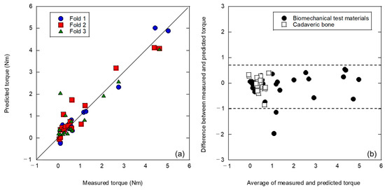
Figure 7.
Analysis results of a three-fold cross validation using a mixed dataset of artificial and cadaveric bones with the introduction of bone density: (a) the relationship between measured and predicted insertion torques; (b) Bland–Altman plot.
Table 3 presents the explanatory variables used in this study. Newly introduced bone density was employed as the explanatory variable with the highest priority, and the highest performance was obtained with SVR using eight variables, which is the largest number to date. However, the peak frequency (1000–5000 Hz), which was previously the most important variable, was given the sixth highest priority by LASSO. Figure 8 shows the performance changes in the (a) coefficient of determination and (b) MSE when introducing SVR for the explanatory variables prioritized by LASSO. In this study, the coefficient of determination, which is the index for optimizing SVR, showed approximately the same value for up to ten variables. However, the MSE showed the lowest value among the six variables when the peak frequency (1000–5000 Hz) was introduced. From these results, it was possible to verify the SVR optimization index. In future work, further performance improvements can be recognized by examining the percentage of cadaveric bone data that should be included in the training data and SVR optimization index. Furthermore, it is possible to introduce explanatory variable selection through sequential selection, without using LASSO. However, in this study, a prediction accuracy in cadaver bones was achieved that was comparable to that of simulated bones by using a uniquely simple selection of explanatory variables by LASSO and SVR optimization, consistent with the coefficient of determination. This achievement is a dramatic improvement over the conventional analysis method, as shown in Figure 3. This analysis method, which can link artificial bone and cadaveric bone, will reduce the number of clinical trials in which data accumulation is difficult, and will contribute to the expansion of implant strength diagnosis through vibration analysis.
Table 3.
Explanatory variables utilized at analysis as shown in Figure 7.
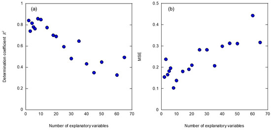
Figure 8.
Performance change in (a) coefficient of determination and (b) MSE when introducing SVR for the explanatory variables prioritized by LASSO.
The limitation of this study is the use of micro-CT, and it is necessary to verify whether equivalent results would be obtained if multislice CT or DEXA results were used. In addition, this study used monoaxial screw analysis, and it was necessary to verify the performance when a polyaxial screw was used. The introduction of artificial bone test data was verified against the background of difficulty in obtaining test data with cadaveric bones. Approximately 35% of the dataset was obtained from cadaveric bones, thereby demonstrating the validity of this method. The reduction in the amount of cadaveric bone data is a future challenge, and the amount of required data is the most essential limitation of the L-RFA for the diagnosis of implant stability. In addition, whether this dataset can be used in other facilities should be verified. If this trained model is available regardless of location, it could be a useful tool for hospitals without experimental infrastructure. If this analysis method is introduced into routine clinical practice, it will improve the accuracy of implant placement procedures and contribute to better patient outcomes. In the future, it is most important to validate the analysis method through clinical trials as it is introduced into clinical practice.
4. Conclusions
In this study, a machine learning analysis was optimized using the L-RFA dataset with artificial bone as teaching data, aiming at a highly accurate prediction of peak insertion torque, equivalent to laboratory-level measurement accuracy, which is an indicator of pedicle screw stability for cadaveric bone installation. In this machine learning-based analysis, many explanatory variables extracted from the laser-induced vibration spectral data obtained from the L-RFA evaluation were predicted by selecting important variables using LASSO and performing a non-linear approximation using SVR. When only the L-RFA evaluation results from the artificial bone were used as teaching data, systematic errors occurred because of the potential differences between the artificial and cadaveric bones. It was found that combining artificial and cadaveric bone data in the teaching data dramatically improved the prediction accuracy and reduced the influence of potential differences between artificial and cadaveric bones. Furthermore, by introducing bone density, which reflects the bone information underlying the clinical data, a high prediction accuracy was achieved, comparable to that achieved with simulated bone alone, as reported in a previous study [10].
In the future, the L-RFA evaluation dataset using cadaveric bones will become a more useful clinical technology if validated using the necessary amount of L-RFA evaluation data. When this technology is realized, it can contribute to the medical technology required to further advance the treatment of musculoskeletal diseases. As society ages, it can be used as a preventive diagnostic technology for bone-fusion defects during surgery. In addition, this technology can be applied not only to medical care, but also to the inspection of buried objects in a wide range of fields, including industrial and social infrastructure, such as concrete bolts. The optimization guidelines for machine learning-based analyses based on the results of this study could be a milestone in L-RFA technology.
Author Contributions
K.M. was responsible for all the procedures, laser system construction, data gathering, analysis, and writing of the manuscript. M.N. (Mitsutaka Nemoto) was responsible for data analysis and took responsibility for the manuscript. A.I. was responsible for data analysis. T.N., M.N. (Masaya Nakamura) and M.M. took responsibility for the clinical tests. D.N. was responsible for bone model preparation, data gathering, and analysis, and took responsibility for conception. All authors have read and agreed to the published version of the manuscript.
Funding
This work was supported by AMED (Grant Numbers JP20hm0102077h0001, JP21hm0102077h0002 and JP22hm0102077h0003).
Institutional Review Board Statement
Not applicable.
Informed Consent Statement
Not applicable.
Data Availability Statement
The datasets used and/or analyzed during this study are available from the corresponding author upon reasonable request.
Conflicts of Interest
The authors declare no conflict of interest.
References
- Deyo, R.A.; Gray, D.T.; Kreuter, W.; Mirza, S.; Martin, B.I. United States trends in lumbar fusion surgery for degenerative conditions. Spine 2005, 30, 1441–1445. [Google Scholar] [CrossRef] [PubMed]
- Weinstein, J.N.; Lurie, J.D.; Olson, P.R.; Bronner, K.K.; Fisher, E.S. United States’ trends and regional variations in lumbar spine surgery: 1992–2003. Spine 2006, 31, 2707–2714. [Google Scholar] [CrossRef] [PubMed]
- Bredow, J.; Boese, C.K.; Werner, C.M.; Siewe, J.; Löhrer, L.; Zarghooni, K.; Eysel, P.; Scheyerer, M.J. Predictive validity of preoperative CT scans and the risk of pedicle screw loosening in spinal surgery. Arch. Orthop. Trauma Surg. 2016, 136, 1063–1067. [Google Scholar] [CrossRef] [PubMed]
- Yagi, M.; Ames, C.P.; Keefe, M.; Hosogane, N.; Smith, J.S.; Shaffrey, C.I.; Schwab, F.; Lafage, V.; Shay, B.R.; Matsumoto, M.; et al. A cost-effectiveness comparisons of adult spinal deformity surgery in the United States and Japan. Eur. Spine J. 2017, 27, 678–684. [Google Scholar] [CrossRef]
- Kwok, A.W.L.; Finkelstein, J.A.; Woodside, T.; Hearn, T.C.; Hu, R.W. Insertional torque and pull-out strengths of conical and cylindrical pedicle screws in cadaveric bone. Spine 1996, 21, 2429–2434. [Google Scholar] [CrossRef]
- Mueller, T.L.; van Lenthe, G.H.; Stauber, M.; Gratzke, C.; Eckstein, F.; Müller, R. Regional, age and gender differences in architectural measures of bone quality and their correlation to bone mechanical competence in the human radius of an elderly population. Bone 2009, 45, 882–891. [Google Scholar] [CrossRef]
- Lei, W.; Wu, Z. Biomechanical evaluation of an expansive pedicle screw in calf vertebrae. Eur. Spine J. 2006, 15, 321–326. [Google Scholar] [CrossRef]
- Ab-Lazid, R.; Perilli, E.; Ryan, M.K.; Costi, J.J.; Reynolds, K.J. Does cancellous screw insertion torque depend on bone mineral density and/or microarchitecture? J. Biomech. 2014, 47, 347–353. [Google Scholar] [CrossRef]
- Mikami, K.; Nakashima, D.; Kikuchi, S.; Kitamura, T.; Hasegawa, N.; Nagura, T.; Nishikino, M. Stability diagnosis of orthopedic implants based on resonance frequency analysis with fiber transmission of nanosecond laser pulse and acceleration sensor. In Proceedings of the Optical Fibers and Sensors for Medical Diagnostics and Treatment Applications XX, San Francisco, CA, USA, 20 February 2020; Volume 11233, p. 1123300. [Google Scholar]
- Nakashima, D.; Mikami, K.; Kikuchi, S.; Nishikino, M.; Kitamura, T.; Hasegawa, N.; Matsumoto, M.; Nakamura, M.; Nagura, T. Laser resonance frequency analysis of pedicle screw stability: A cadaveric model bone study. J. Ortho. Res. 2021, 39, 2474–2484. [Google Scholar] [CrossRef]
- Kikuchi, S.; Mikami, K.; Nakashima, D.; Kitamura, T.; Hasegawa, N.; Nishikino, M.; Kanaji, A.; Nakamura, M.; Nagura, T. Laser Resonance Frequency Analysis: A Novel Measurement Approach to Evaluate Acetabular Cup Stability During Surgery. Sensors 2019, 19, 4876. [Google Scholar] [CrossRef]
- Kurahashi, S.; Mikami, K.; Kitamura, T.; Hasegawa, N.; Okada, H.; Kondo, S.; Nishikino, M.; Kawachi, T.; Shimada, Y. Demonstration of 25-Hz-inspection-speed laser remote sensing for internal concrete defects. J. Appl. Remote Sens. 2018, 12, 15009. [Google Scholar] [CrossRef]
- Mikami, K.; Hasegawa, N.; Kitamura, T.; Okada, H.; Kondo, S.; Nishikino, M. Characterization of laser-induced vibration on concrete surface toward highly efficient laser remote sensing. Jpn. J. Appl. Phys. 2020, 59, 076502. [Google Scholar] [CrossRef]
- Mishra, S.; Kumar, M.; Mishra, L.; Mohanty, R.; Nayak, R.; Das, A.C.; Mishra, S.; Panda, S.; Lapinska, B. Fractal Dimension as a Tool for Assessment of Dental Implant Stability—A Scoping Review. J. Clin. Med. 2022, 11, 4051. [Google Scholar] [CrossRef] [PubMed]
- Meredith, M.; Alleyne, D.; Cawley, P. Quantitative determination of the stability of the implant-tissue interface using resonance frequency analysis. Clin. Oral Impl. Res. 1996, 7, 261–267. [Google Scholar] [CrossRef] [PubMed]
- Nakashima, D.; Ishii, K.; Matsumoto, M.; Nakamura, M.; Nagura, T. A study on the use of the Osstell apparatus to evaluate pedicle screw stability: An in-vitro study using micro-CT. PLoS ONE 2018, 13, e0199362. [Google Scholar] [CrossRef] [PubMed]
- Georgiou, A.P.; Cunningham, J.L. Accurate diagnosis of hip prosthesis loosening using a vibrational technique. Clin. Biomech. 2001, 16, 315–323. [Google Scholar] [CrossRef]
- Pastrav, L.C.; Jaecques, S.V.N.; Jonkers, I.; Van der Parre, G.; Mulier, M. In vivo evaluation of a vibration analysis technique for the per-operative monitoring of the fixation of hip prostheses. J. Orthop. Surg. Res. 2009, 4, 10. [Google Scholar] [CrossRef] [PubMed]
- Henys, P.; Capek, L.; Fencl, J.; Prochazka, E. Evaluation of acetabular cup initial fixation by using resonance frequency analysis. Proc. Inst. Mech. Eng. Part H J. Eng. Med. 2015, 229, 3–8. [Google Scholar] [CrossRef]
- Mikami, K.; Nemoto, M.; Nagura, T.; Nakamura, M.; Matsumoto, M.; Nakashima, D. Machine Learning-Based Diagnosis in Laser Resonance Frequency Analysis for Implant Stability of Orthopedic Pedicle Screws. Sensors 2021, 21, 7553. [Google Scholar] [CrossRef]
- Paik, H.; Dmitriev, A.E.; Lehman, R.A., Jr.; Gaume, R.E.; Ambati, D.V.; Kang, D.G.; Lenke, L.G. The biomechanical effect of pedicle screw hubbing on pullout resistance in the thoracic spine. Spine J. 2012, 12, 417–424. [Google Scholar] [CrossRef]
- Matsukawa, K.; Yato, Y.; Kato, T.; Imabayashi, H.; Asazuma, T.; Nemoto, K. In vivo analysis of insertional torque during pedicle screwing using cortical bone trajectory technique. Spine 2014, 39, E240–E245. [Google Scholar] [CrossRef] [PubMed]
- Daftari, T.K.; Horton, W.C.; Hutton, W.C. Correlations between screw hole preparation, torque of insertion, and pullout strength for spinal screws. J. Spinal Disord. 1994, 7, 139–145. [Google Scholar] [CrossRef] [PubMed]
- Nakashima, D.; Ishii, K.; Nishiwaki, Y.; Kawana, H.; Jinzaki, M.; Matsumoto, M.; Nakamura, M.; Nagura, T. Quantitative CT-based bone strength parameters for the prediction of novel spinal implant stability using resonance frequency analysis: A cadaveric study involving experimental micro-CT and clinical multislice CT. Eur. Radiol. Exp. 2019, 3, 1. [Google Scholar] [CrossRef]
- Santosa, F.; Symes, W.W. Linear inversion of band-limited reflection seismograms. J. Sci. Stat. Comput. 1986, 7, 1307–1330. [Google Scholar] [CrossRef]
- Tibshirani, R. Regression shrinkage and selection via the Lasso. J. R. Statist. Soc. B 1996, 58, 267–288. [Google Scholar] [CrossRef]
- Vapnik, V. Pattern recognition using generalized portrait method. Autom. Remote Control 1963, 24, 774–780. [Google Scholar]
- Boser, B.E.; Guyon, I.M.; Vapnik, V. A training algorithm for optimal margin classifiers. In Proceedings of the Fifth Annual Workshop on Computational Learning Theory, Pittsburgh, PA, USA, 27–29 July 1992; pp. 144–152. [Google Scholar]


Disclaimer/Publisher’s Note: The statements, opinions and data contained in all publications are solely those of the individual author(s) and contributor(s) and not of MDPI and/or the editor(s). MDPI and/or the editor(s) disclaim responsibility for any injury to people or property resulting from any ideas, methods, instructions or products referred to in the content. |
© 2023 by the authors. Licensee MDPI, Basel, Switzerland. This article is an open access article distributed under the terms and conditions of the Creative Commons Attribution (CC BY) license (https://creativecommons.org/licenses/by/4.0/).