Multi-Objective Parameter Optimization of Submersible Well Pumps Based on RBF Neural Network and Particle Swarm Optimization

Abstract

In order to improve the hydraulic performance of a submersible well pump, steady and transient simulations were carried out based on ANSYS CFX software. The head and efficiency of the submersible well pump under standard operating conditions were taken as the optimization objectives, and the impeller outlet placement angle, outlet width, and vane wrap angle were selected as the optimization variables using the Plackett-Burman experimental design method. The RBF neural network training samples were constructed using the uniform experimental design method to build a hydraulic performance prediction model for the submersible well pump, and a multi-objective particle swarm optimization was used to solve the model and obtain the Pareto optimal solution set. Using the head and efficiency of the initial model as the boundary, the Pareto optimal solution and the corresponding structural parameters are sought. After the optimization, the head of the individual with the better head is increased by about 2.65 m, and the efficiency of the individual with the better efficiency is increased by about 2.3 percentage points compared with that of the initial model. The pressure gradient in the impeller flow channel is more obvious, the work capacity is significantly improved, the vortex area of the spatial guide vane is smaller, the flow line is more regular, and the pressure pulsation amplitude at the inlet and outlet of the impeller and the spatial guide vane is significantly reduced.

1. Introduction

With the application and development of numerical simulation and optimal design techniques in the field of pump research, the performance of submersible well pumps has been improved to a certain extent, but it still cannot meet the needs on some specific occasions due to certain limitations on efficiency and the pump head. The impeller, as the core hydraulic component of well submersible pumps, has an important influence on the hydraulic performance of the pump. For this reason, it is of great research significance to develop the optimal design of impeller hydraulics to improve the comprehensive performance of submersible well pumps.

At present, scholars at home and abroad have applied approximate prediction models and intelligent optimization algorithms to some pump models to optimize the design and improve the performance of the pump. Zhang et al. [1] investigated the hydrodynamic characteristics of a single-stage centrifugal pump with an induced wheel at the inlet and a radial guide vane (RGV) at the outlet subjected to the changing law of timing effects and found that there exists an optimal position that can both increase the pump head and efficiency and reduce the intensity of pressure pulsation. Lai et al. [2], in order to investigate the timing effects of centrifugal pumps, based on the k-omega shear stress transport model for 3D numerical calculations, found that the optimum diffuser installation angle is 25 degrees when the total pressure loss and radial force acting on the impeller are the smallest. Tan et al. [3] investigated the timing effect of the impeller in a five-stage centrifugal pump and the superposition effect between the pump stages induced by the timing effect and found that the head and efficiency of the pump did not vary much, while the vibration frequency and amplitude varied considerably. Gu et al. [4] conducted an investigation of the vane diffuser relative to the circumference of the circular housing at different timing positions, and based on the minimum entropy generation theory of computational fluid dynamics, the flow loss visualization method was used to describe the losses caused by the timing positions. Yuan Shouqi et al. [5] used the IS50-32-160 low specific speed pump as a research model and adopted an optimization method combining a Kriging approximation model and a genetic algorithm to optimize the main structural parameters of the impeller, which not only improved the efficiency but also reduced the intensity of the pressure pulsation of the pump. Lei Mingchuan [6] combined artificial networks with genetic algorithms to design a multi-objective optimization method for the impeller of a mixed-flow pump, which improved the external characteristics of the pump and effectively curbed the humping phenomenon of the external characteristics curve. Wang Chunlin et al. [7] took a high specific speed pump as the research object and combined a neural network and optimization algorithm to optimize the head and efficiency of the pump and improve its hydraulic performance. Zhao Weiguo et al. [8] optimized the efficiency of a centrifugal pump under standard conditions based on a neural network and genetic algorithm. The results showed that the efficiency of the centrifugal pump under standard conditions increased by 4.41 percentage points and the head increased by 2.63 m. Reasonable design improvements were also made to the worm casing to address the problem of insignificant improvement in the remaining operating conditions. Liao Fu et al. [9] used the pump head, efficiency, and cavitation margin as the optimization objectives and applied genetic algorithms to solve them, making improvements to the previous design methods for low specific speed centrifugal pumps while also providing a reference basis for subsequent designs. Jiang Wenzhi et al. [10] combined the BP neural network genetic algorithm to optimize the centrifugal pump and improve the hydraulic performance of the pump. Wang Chunlin et al. [11] applied a neural network and the NSGA-II genetic algorithm to slurry pumps to achieve the optimal design of efficiency as well as the high efficiency zone of this pump. Tao Ran et al. [12] optimized the vane inlet and outlet angles based on a genetic algorithm with efficiency as the optimization objective, which led to a 4.5 percentage point increase in pump efficiency and a significant expansion of the high efficiency zone, as well as a 0.83 m increase in the pump head. Li Qimin et al. [13] optimized a fuel pump using a genetic algorithm combined with an adaptive weighting method, with impeller structural parameters as the optimization variables and volumetric efficiency and outlet flow rate as the optimization objectives, which resulted in a 3.9 percentage point increase in outlet flow rate and a 0.53 percentage point increase in volumetric efficiency. Wang Chunlin et al. [14] took a double-vane sewage pump as the research object and used a combination of neural network and particle swarm optimization to optimize the design, and after experimental verification, the optimized pump head efficiency was improved to some extent. Dong Min et al. [15] took a model of a low specific speed pump as the research object, with the stability of the operating process, anti-cavitation performance, and energy loss as the optimization targets, and used a genetic algorithm to calculate the solution. After optimization, the pump pressure pulsation amplitude was reduced, and the stability improved to some extent. Ye Daoxing et al. [16] used a cyclone pump as the research object, with the width of the non-vane cavity, the number of vanes, and the vane outlet width as the optimization variables and the efficiency and vane surface shear stress as the optimization objectives. They used a genetic algorithm and Kriging model to calculate the solution, which improved efficiency and reduced the average vane shear stress. Tong Zheming et al. [17] selected three optimization variables, namely impeller outlet width, diameter, and angle, and combined the Latin hypercube sampling method, BP neural network, and NSGA-III algorithm to optimize a model of a low specific speed centrifugal pump with pump head and efficiency as the optimization objectives. Jiang Bingxiao et al. [18] optimized the geometric parameters of the vane profile of a centrifugal pump based on an intelligent algorithm, and the numerical simulation and experimental values of pump head efficiency were improved after optimization. Hao Zongrui et al. [19] studied a water jet propulsion pump with lift resistance ratio and pressure as the optimization objectives and carried out optimization based on an improved particle swarm optimization algorithm, after which the lift resistance ratio was improved by 14.7 percentage points and the minimum pressure was increased by 20%. Wang Mengcheng et al. [20] took a mixed-flow pump as the optimization object, selected the vane load as the optimization variable, 0.7 times the standard operating condition to 1.1 times the standard operating condition high efficiency zone as the optimization objective, and used the Kriging approximation model and NSGA-II algorithm for optimization. However, most of the optimization is carried out by a genetic algorithm, and there is less research on the application of neural network prediction models combined with multi-objective particle swarm optimization to the optimal design of submersible well pumps.

The research and analysis of pump performance optimization mainly include the following: studying the impact of a single factor on pump performance; optimizing the theoretical formula of pump performance; applying experimental design methods to optimize pump performance; combining experimental design and an approximate prediction model [21]; and using intelligent optimization algorithms to directly search for the optimal computational solution. The experimental design method can analyze the degree of influence of the optimization parameters on the optimization target [22]; the approximate prediction model can reflect the relationship between the optimization parameters and the optimization target with high accuracy, mainly using an artificial neural network, the response surface method [23], the Kriging model, etc.; and the intelligent optimization algorithm can seek the optimal solution with high accuracy and efficiency. Based on the above analysis methods, this paper takes the 200QJ20 submersible well pump as the research object, establishes the performance prediction model of the submersible well pump through the RBF neural network, and uses the multi-objective particle swarm optimization algorithm to obtain the Pareto optimal solution set. The external characteristic data of the initial model is used as the boundary to find the best solution for the pump head and efficiency. The improvement of this research method provides a basis and reference for improving the hydraulic performance of the submersible well pump, improving its efficiency, and developing new pump models.

2. Numerical Simulation

2.1. Governing Equation

Regardless of the complexity of the fluid flow in the pump, the basic laws of physics must be obeyed, of which the laws of conservation of mass, momentum, and energy are the three most basic conservation laws in fluid flow problems.

(1)

The continuity equation

The continuity equation, also called the mass conservation equation, has the following specific expression:

$$\frac{\partial \rho }{\partial t}+\frac{\partial (\rho u_i)}{\partial t}=0$$

(1)

where $u_i$ is the fluid velocity component and $\rho$ is the fluid density (kg/m³).

For steady flow, the above equation can be replaced by:

$$\frac{\partial (\rho u_i)}{\partial t}=0$$

(2)

For incompressible fluids, the equation can be changed to:

$$\frac{\partial u_i}{\partial x_i}=0$$

(3)

where $x_i$ is the coordinate component and $i$ = 1, 2, 3.

(2)

Momentum equation

The momentum equation, namely the N-S equation, for incompressible viscous fluids has a specific expression as follows:

$$\frac{\partial u_i}{\partial t}+u_j\frac{\partial u_i}{\partial x_j}=F_i-\frac{1}{\rho }\frac{\partial P}{\partial x_i}+\upsilon \frac{{\partial }^2{u}_i}{\partial x_i\partial x_j}$$

(4)

where $u_j$ is the fluid velocity component, $x_j$ is the coordinate component, $j$ = 1, 2, 3, $F_i$ is the mass force (N), $P$ is the pressure (Pa), $\rho$ is the fluid density (kg/m³), and $\upsilon$ is the kinematic viscosity coefficient.

(3)

Energy conservation equation

The law of conservation of energy states that the total amount of energy always remains the same, regardless of how it changes during the process of transfer and conversion. For incompressible fluids, the specific expression is as follows:

$$\frac{D}{Dt}(\frac{1}{2}{u}_i{u}_i)=u_i{F}_{xi}+\frac{1}{\rho }\frac{\partial (m_{ji}{u}_i)}{\partial x_j}-\frac{1}{\rho }\frac{\partial (p{u}_i)}{\partial x_j}+\frac{p}{\rho }\frac{\partial u_i}{\partial x_j}-\frac{m_{ij}}{\rho }\frac{\partial u_i}{\partial x_j}$$

(5)

where $m_{ij}$ is the viscous stress tensor.

For a fluid microcluster per unit volume, the specific expression for the increment of internal energy per unit time is:

$$\frac{De}{Dt}=q-\frac{1}{\rho }\frac{\partial q_i}{\partial x_i}+\frac{\Phi }{\rho }-\frac{p}{\upsilon }\frac{\partial u_i}{\partial x_i}$$

(6)

where $e$ is the internal energy per unit mass, $q$ is the heat gained per unit of volume, $q_i$ is the thermal energy per unit of time volume, and $\Phi$ is the dissipation function, which can be expressed as $\Phi =m_{ji}\frac{\partial u_i}{\partial x_j}$.

From this, the energy equation for an incompressible viscous fluid is given by:

$$\frac{D}{Dt}(e+\frac{1}{2}{u}_i{u}_i)=Q+u_i{F}_{xi}-\frac{1}{\rho }\frac{\partial q_i}{\partial x_i}+\frac{1}{\rho }\frac{\partial (m_{ji}{u}_i)}{\partial x_j}-\frac{1}{\rho }\frac{\partial (p{u}_i)}{\partial x_j}$$

(7)

2.2. The Selection of the Realizable k-ε

Turbulence models are commonly used to describe the changing laws of fluid flow within a submersible well pump and can be divided into Reynolds stress models and eddy viscosity models. The eddy viscosity model can be subdivided into a zero-equation model, a one-equation model, and a two-equation model. The two-equation models are more mature and well developed, and the common two-equation models include the standard k-ε model, the RNG k-ε model, and the Realizable k-ε model. As the Realizable k-ε model satisfies the constraints on Reynolds stress, its advantage is its ability to predict planar and circular jet diffusion effects more accurately. Moreover, it also performs well for rotating flows, boundary layer flows with strong inverse pressure gradients, flow separation, and secondary flows. Therefore, the Realizable k-ε model is used in this paper for simulation calculations. Its specific expression is shown in the following equation:

$$\frac{\partial (\rho k)}{\partial t}+\frac{\partial (\rho k{\mu }_i)}{\partial x_i}=\frac{\partial }{\partial x_j}[(\mu +\frac{{\mu }_t}{{\sigma }_{\tau }})\frac{{\partial }_k}{\partial x_j}]+G_k-\rho \epsilon$$

(8)

${\mu }_t$ and $C_{\mu }$ can be calculated using the following formula:

$${\mu }_t=\rho C_{\mu }\frac{k^2}{\epsilon }$$

(9)

$$C_{\mu }=\frac{1}{A_0+A_s{U}^{\ast }\raisebox{1ex}{$k$}\!\left/ \!\raisebox{-1ex}{$\epsilon $}\right.}$$

(10)

where $A_0=4.0$, $A_s$ = $\sqrt{6}\cos \varphi$, $\varphi =\frac{1}{3}{\cos }^{-1}(\sqrt{6}W)$, $W=\frac{E_{ij}{E}_{ijk}{E}_{kj}}{\sqrt{(E_{ij}{E}_{ij})}}$, $E_{ij}=\frac{1}{2}(\frac{\partial {\mu }_i}{\partial x_j}+\frac{\partial {\mu }_j}{\partial x_j})$, $U^{\ast }=\sqrt{E_{ij}{E}_{ij}+{\Omega }_{ij}{\Omega }_{ij}}$, ${\Omega }_{ij}={\Omega }_{ij}-2{\epsilon }_{ijk}{\omega }_k$, and ${\Omega }_{ij}={\Omega }_{ij}-{\epsilon }_{ijk}{\omega }_k$.

$$\frac{\partial (\rho \epsilon )}{\partial t}+\frac{\partial (\rho \epsilon {\mu }_i)}{\partial x_i}=\frac{\partial }{\partial x_j}[(\mu +\frac{{\mu }_t}{{\sigma }_{\epsilon }})\frac{{\partial }_{\epsilon }}{\partial x_j}]+\rho C_1{E}_{\epsilon }{G}_k-\rho C_2\frac{{\epsilon }^2}{k+\sqrt{\upsilon \epsilon }}$$

(11)

where ${\sigma }_k=1.0$, ${\sigma }_{\tau }=1.2$, $C_2=1.9$, $C_1=\max (0.43,\frac{\eta }{\eta +5})$, $\eta =2{(E_{ij}{E}_{ij})}^{\raisebox{1ex}{$1$}\!\left/ \!\raisebox{-1ex}{$2$}\right.}\frac{k}{\epsilon }$, and $E_{ij}=\frac{1}{2}(\frac{\partial {\mu }_i}{\partial x_j}+\frac{\partial {\mu }_j}{\partial x_i})$.

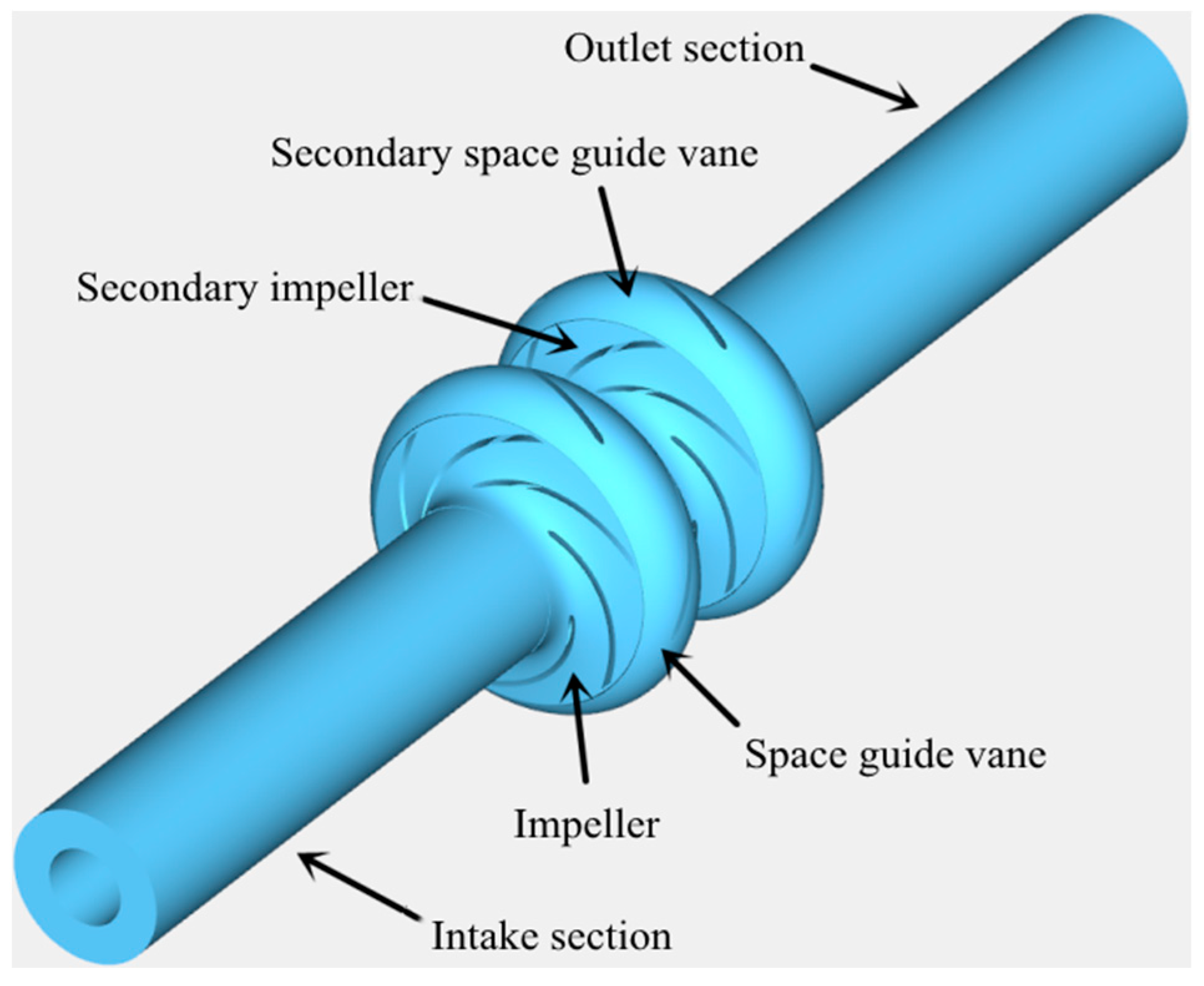
2.3. Geometric Model

The basic hydraulic design parameters of a multi-stage 200QJ20 submersible well pump are: rated flow Q_d = 20 m³/h; single-stage head H_s = 13.5 m; rotational speed n = 2850 r/min; specific rotation n_s = 110.09. The number of impeller blades on the original model pump is Z₁ = 6. The six blades are evenly distributed in the direction of the suction port; the blades rotate counterclockwise; and the surface of the flow channel is smooth. Blade inlet thickness is 2 mm, and blade outlet thickness is 2.5 mm. The original pump space guide vane number is Z₂ = 5, and the blade is a twisted vane. Based on CFturbo2020 software for submersible well pump inlet and outlet sections, impellers, and space guide vane components, establish a fluid calculation domain model. The length of the inlet and outlet sections was set to 4 times the inlet and outlet diameters in order to allow the fluid to develop fully. The inlet of the first stage of the multi-stage submersible pump for wells uses non-pre-rotating flow, and the inlet after the second stage uses rotating flow, so the internal flow pattern of the second stage can represent the subsequent flow patterns. Considering the computer numerical simulation solution time, a two-stage submersible pump model is established in the paper for analysis. The computational domain model obtained from the assembly is shown in Figure 1.

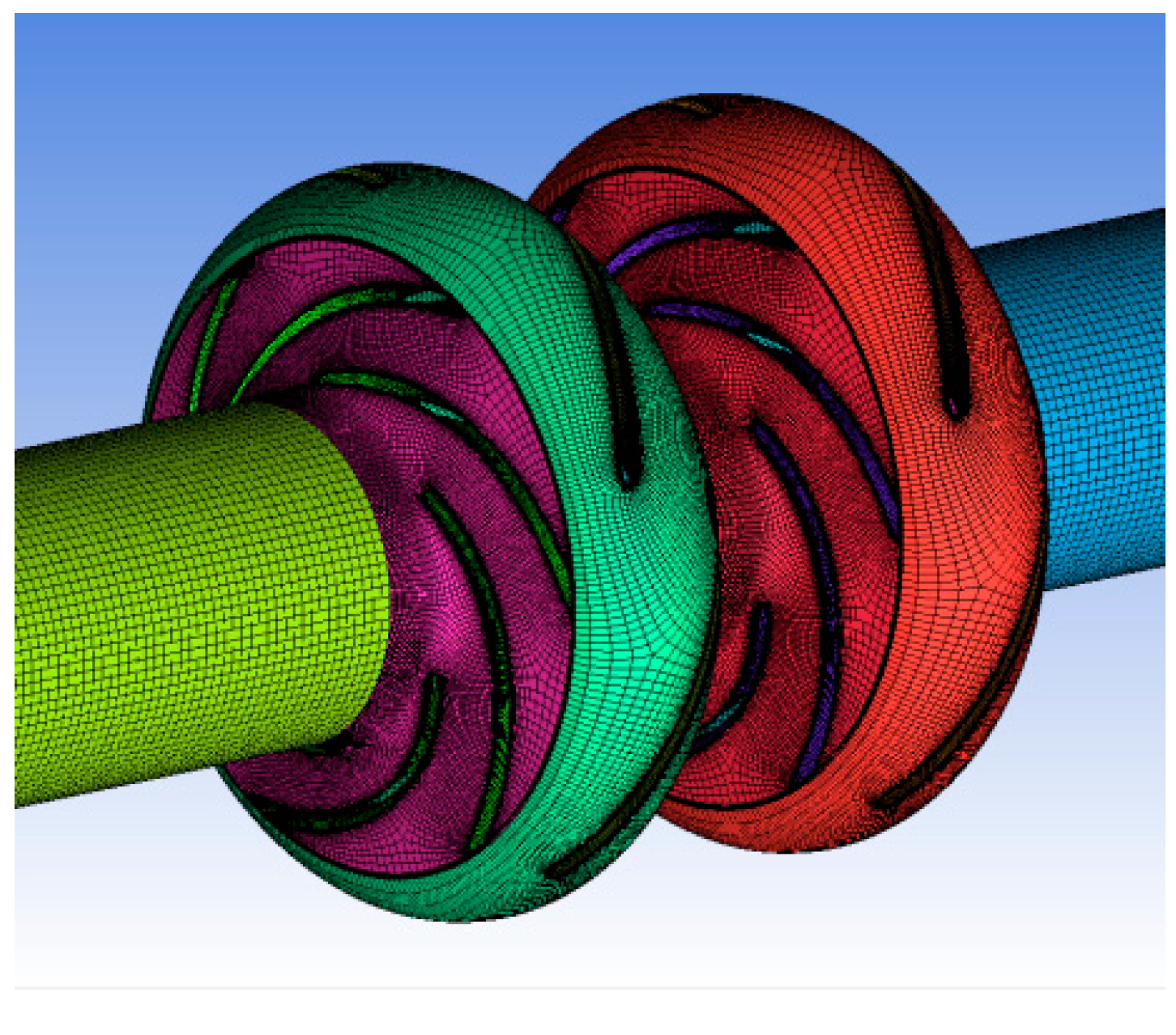
2.4. Meshing and Irrelevance Analysis

Mesh delineation is the basis for subsequent simulation calculations, and the quality of the mesh will have a direct impact on the simulation results. Unstructured meshes are more randomly distributed, simple and fast to generate, flexible, and can be adapted to a variety of complex geometries, but there is also the problem of poor quality local meshing, resulting in poor overall mesh quality, large quantities, and a long computational solution time. The structured mesh requires a block topology of the model, which will lead to a more complex and time-consuming mesh division, but considering its regular node distribution, it can better save computational solution time and achieve convergence accuracy faster. Therefore, this paper adopts the structured meshing method for meshing. Figure 2 and Figure 3 show the meshing results.

In order to reduce the influence of the number of grids on the accuracy of the calculation, a grid-independent analysis was carried out, as shown in

Table 1. Grid independence analysis.

Program Number	Number of Full Runner Grids (pc)	Relative Head	Relative Efficiency
1	1,103,596	1.0152	1.0123
2	2,563,487	1.0000	1.0000
3	4,016,349	0.9956	0.9963
4	5,538,964	0.9931	0.9946

. The head and efficiency of Program2 are taken as unit 1, and the head and efficiency of all other Programs are compared with Program2. When the number of grids in the full flow channel reaches 4 million, the head and efficiency tend to stabilize, and the relative head error between Program 3 and Program 4 is 0.25% and the relative efficiency error is 0.17%. In view of the computer configuration and calculation time, the division of Program 3 was finally determined as the standard for dividing all models. The following describes the different quality metrics of this model: The average aspect ratio refers to the average of the aspect ratios of all the grid cells in the whole model. In this model, the mean aspect ratio is 1.91, which indicates that most of the grid cells have relatively close aspect ratios and that the overall shape of the grid is more balanced. The mean warping factor indicates the degree of deformation of the shape of the grid cells. In this model, the average warping factor is 0.002, which indicates that most of the grid cells are relatively well shaped with no obvious deformation or distortion. The maximum top angle, which refers to the largest angle in the grid cell, ranges from 60° to 130°. This indicates that the grid cells are reasonably shaped, with no angles that are too sharp or too flat. The tilt, which is used to assess the degree of deformation of the grid cells, ranges from 0 to 0.75. More than 80% of the grid cells have tilts less than 0.5, which indicates that most of the cells are relatively stable and do not deform excessively. The orthogonality coefficient is used to measure the perpendicularity of the grid lines to their neighbors and has an average value of 0.89. The fact that more than 83% of the cells have orthogonality coefficients greater than 0.75 indicates that the majority of the cells have good orthogonality, and the grid lines are relatively perpendicular. Taken together, the division of Program 3 seems to perform better in most of the quality indicators when computer configuration and computation time are considered and can be used as a criterion for dividing all models.

2.5. Resolving Schemes

The numerical calculations are based on ANSYS CFX18.0, and the settings are made in the CFX pre-processing module. The settings for the steady calculation are as follows: impeller speed is set to 2850 r/min, inlet is set to one atmosphere, outlet is mass flow, flow rate is 20 L/min, fluid density is 998.2 kg/m³, dynamic viscosity is 1.003 × 10⁻³ Pa·s, interaction surface is set to “Frozen Rotor”, overall turbulence intensity is 5%, and convergence accuracy is 10⁻⁴. For transient calculations, the interaction surface is changed to “Transient Rotor Stator” and the total time is set to 0.10526316 s with a time step of 0.0002339 s (one step every 4°), and the results are output every five time steps in order to stabilize the transient calculation. Once completed, the results of the last cycle were used for data analysis.

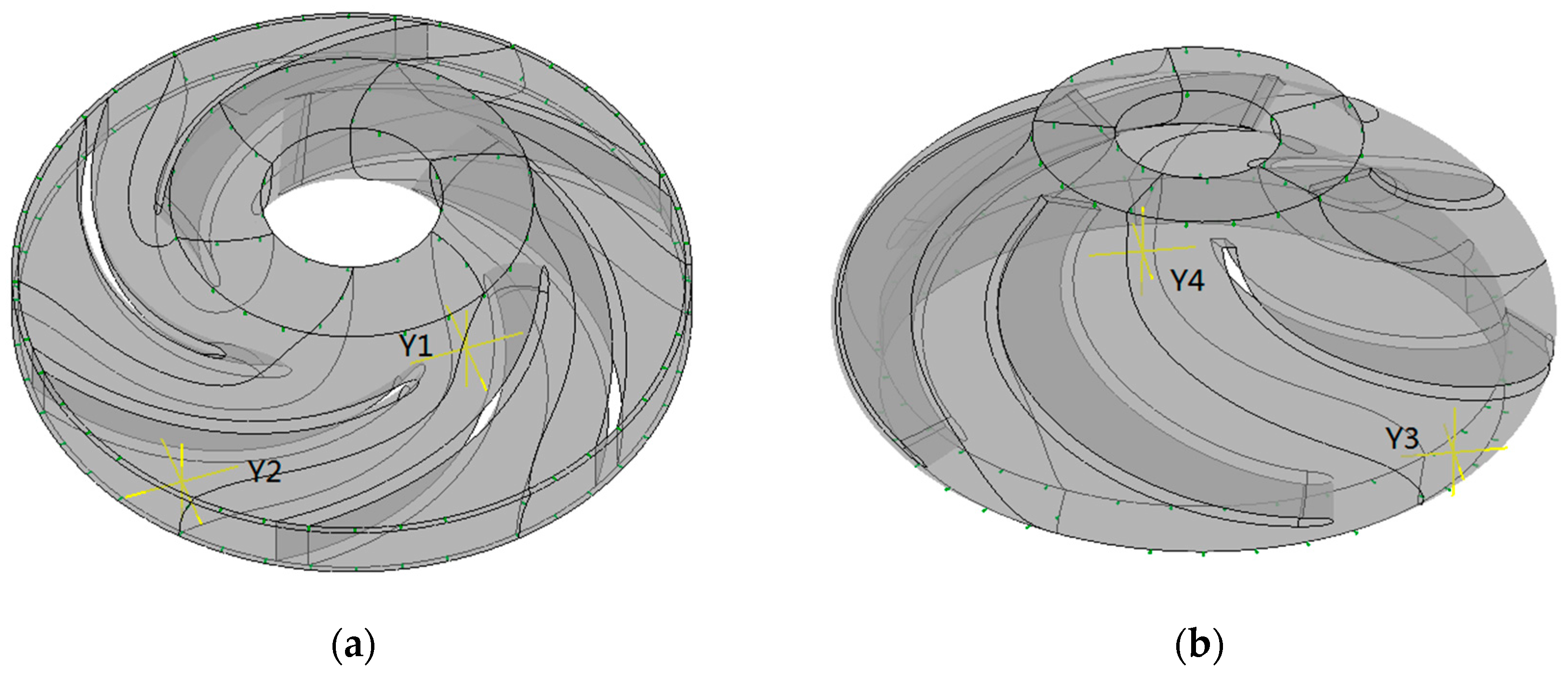
2.6. Monitoring Point Setup

In order to analyze the pattern of pressure pulsation changes, monitoring points Y1 and Y2 are arranged in the secondary impeller runners near the central position of the inlet and outlet area, and monitoring points Y3 and Y4 are arranged in the secondary space guide runners near the central position of the inlet and outlet area, as shown in Figure 4.

To make the calculation more practical and general, the dimensionless pressure pulsation coefficient C_P is introduced and calculated as follows:

$$C_P=\frac{p-\overline{p}}{\frac{1}{2}\rho u_2{}^2}$$

(12)

where p indicates the pressure value at the position of the monitoring point at a certain moment, $\overline{p}$ indicates the average value of the pressure at the monitoring point during a cycle, ρ indicates the density of the medium conveyed by the pump, and u₂ indicates the impeller outlet circumferential velocity.

3. Comparison of Theoretical Simulation and Performance Tests

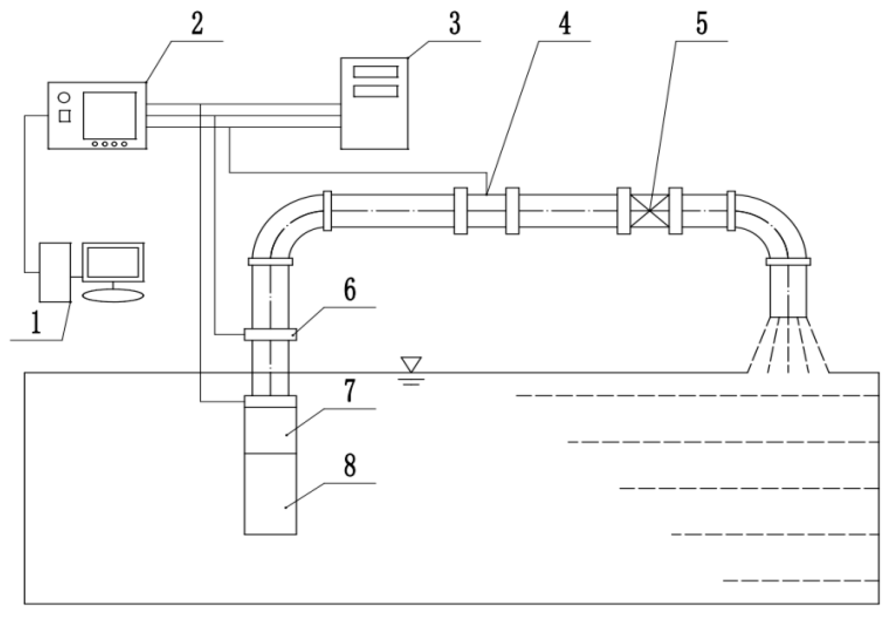
3.1. Test Platform Construction

In order to verify the reasonableness and accuracy of the model and simulation parameter settings, the submersible well pump performance experimental test platform was built, and the test principle is shown in Figure 5. It mainly includes the CYB type intelligent pressure transmitter, the LDTH type DN400 electromagnetic flow meter (accuracy ± 0.3%), the ZDLM type electric control valve, and the 381LS type electronic electric actuator.

Before the start of the test, put the submersible well pump into the water. Running the submersible well pump makes the pipeline discharge air, so close the valve. The experiment starts with zero flow, and then the valve opening is gradually increased. In the process of increasing the flow from small to large, the flow rate is stable during the corresponding data collection. In standard working conditions, more data points are collected, while in small and large flow conditions, a relatively small number of data points are collected.

Pump performance test schematic diagram. (1) Computer; (2) data acquisition instrument; (3) distribution cabinet; (4) DN400 electromagnetic flow meter; (5) ZDLM type electric control valve; (6) CYB type intelligent pressure transmitter; (7) pump body; (8) electric motor.

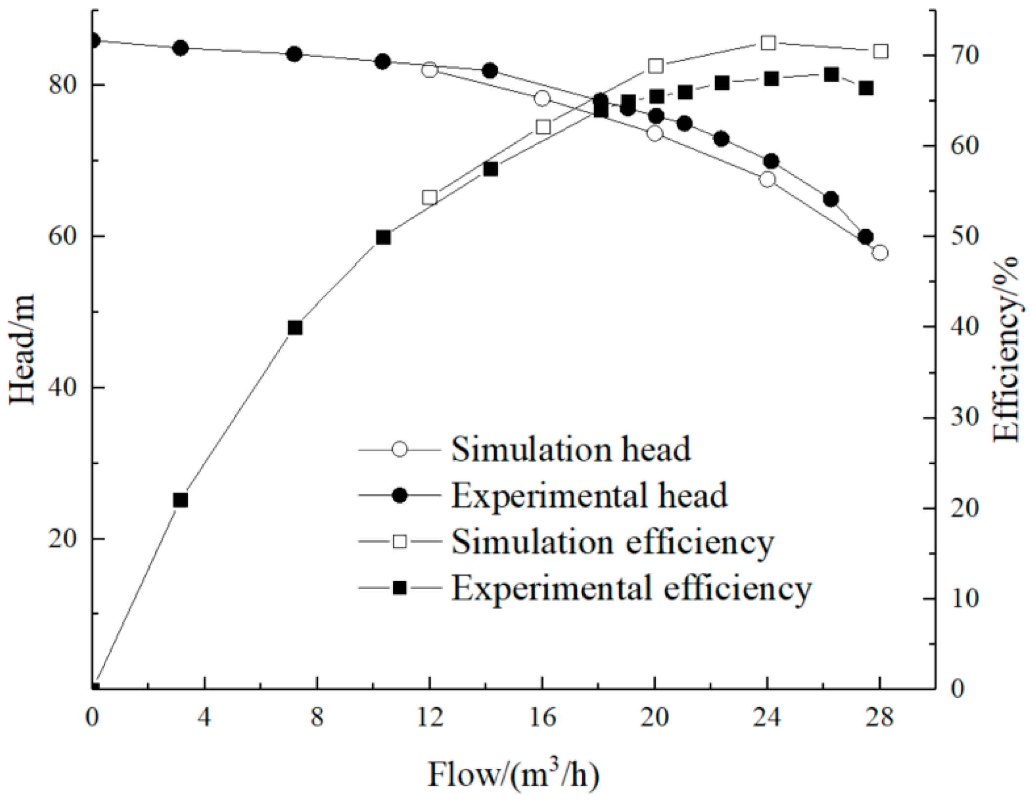
3.2. Comparative Analysis of Theoretical Simulations and Performance Experiments

Usually, in fluid simulation, the selection of working conditions near the rated flow rate for simulation can improve the calculation accuracy and stability of the results. The common practice is to select a range of rated flow, which is usually simulated between 0.6 and 1.4 times the standard condition. Figure 6 shows the comparison between the numerical simulation’s external characteristics and the experimental external characteristics curve. Since the model is a two-stage model and the experimental model is a six-stage model, the two-stage data obtained from the simulation needs to be converted to a six-stage model. Under standard working conditions, the experimental test head and efficiency are basically consistent with the results of the numerical simulation. The simulated head is slightly lower than the experimental head, and the maximum error does not exceed 3%. At the same time, the simulated efficiency is slightly higher than the experimental efficiency, and the maximum error does not exceed 3.4%. This shows that the simulation results can completely replace the experimental test results and can predict the actual performance of the submersible well pump, which provides a basis for further simulation. The main reasons for the errors between simulation and experimental tests are that one is influenced by the configuration of the computer and amount of meshing, and the other is influenced by the simplification of the simulation model.

4. Multi-Objective Optimization

4.1. Significance Analysis of Influencing Factors

There are many geometric parameters affecting the hydraulic performance of submersible pumps for wells, including the import and export placement angle, import and export diameter, outlet width, vane wrap angle, timing position, and other influencing factors. The impeller inlet and outlet diameters will have an impact on the assembly of the space guide vane and the radial dimensions of the submersible well pump, so they are not considered target parameters for this design optimization. The Plackett-Burman experimental design module of Design Expert 12.0 software was used to perform significance analysis on the impeller inlet and outlet placement angles, outlet width, blade wrap angle, and timing position. A multiple of 0.8 of the original model variable parameters was taken as the low level (−1), and a multiple of 1.2 of the original model variable parameters was taken as the high level (+1). For the temporal position, no rotation of the secondary impeller relative to the first impeller (i.e., 0° rotation of the secondary impeller) was taken as the low level (−1), and one-half rotation of the secondary impeller by one-half of the blade angle (i.e., 30° rotation of the secondary impeller) was taken as the high level (+1). Six sets of dummy factors, X₆, X₇, X₈, X₉, X₁₀, and X₁₁, were added as error analysis.

Table 2. Influencing factors and levels.

Variables	Parameter Name	Unit	Low Level	High Level
X1	Imported placement angle β1	/°	17	26
X2	Exit placement angle β2	/°	21	32
X3	Outlet width b2	/mm	8	12
X4	Blade wrap angle φ	/°	77	116
X5	Impeller timing position	/°	0	30
X6~X11	Virtual factors	—	—	—

shows the names and level settings of the influencing factors. Twelve sets of tests were required, and the distribution of the high- and low-level arrangements of the influencing factors is shown in

Table 3. Plackett-Burman experimental design permutation distribution.

Serial Number	Imported Placement Angle β1	Exit Placement Angle β2	Outlet Width b2	Blade Wrap Angle φ	Impeller Timing Position
1	1	−1	1	1	1
2	−1	1	1	−1	1
3	1	−1	−1	−1	1
4	−1	−1	−1	−1	−1
5	−1	−1	1	−1	1
6	−1	−1	−1	1	−1
7	1	1	−1	1	1
8	1	−1	1	1	−1
9	−1	1	−1	1	1
10	−1	1	1	1	−1
11	1	1	1	−1	−1
12	1	1	−1	−1	−1

.

According to the Plackett-Burman experimental design, the distribution order of the high and low levels of each influencing factor was arranged, and the specific values of the high and low levels corresponding to each influencing factor were substituted into Table 3. The 12 sets of structural parameters and a model of the 12 sets of submersible well pumps were created in CFturbo software. The model was imported into ANSYS19.2 CFX software for 12 sets of simulations, and the corresponding head and efficiency for each set of solutions were obtained as shown in

Table 4. Plackett-Burman experimental design and numerical simulation results.

Serial Number	Imported Placement Angle β1	Exit Placement Angle β2	Outlet Width b2	Blade Wrap Angle φ	Impeller Timing Position	Lift	Efficiency
1	26	21	12	116	30	24.6248	77.9006
2	17	32	12	77	30	26.8351	68.1091
3	26	21	8	77	30	22.3482	75.5079
4	17	21	8	77	0	22.7505	75.1389
5	17	21	12	77	30	25.7977	69.4718
6	17	21	8	116	0	20.1328	78.2832
7	26	32	8	116	30	20.9667	77.3769
8	26	21	12	116	0	24.4402	77.9071
9	17	32	8	116	30	21.5795	76.9954
10	17	32	12	116	0	25.5931	75.923
11	26	32	12	77	0	27.0253	68.0776
12	26	32	8	77	0	23.176	74.292

.

Table 5. Significant analysis of influencing factors for the pump head.

Factors	Sum of Squares (%)	Coefficient Assessment	Standard Error	p-Value
Imported placement angle β1	0.0010	−0.0090	0.1078	0.9365
Exit placement angle β2	2.15	0.4235	0.1078	0.0077
Outlet width b2	45.48	1.95	0.1078	<0.0001
Blade wrap angle φ	9.36	−0.8830	0.1078	0.0002
Impeller timing position	0.0777	−0.0805	0.1078	0.4834

demonstrates the degree of influence of the main geometric parameters on the head. As can be seen from the table, the percentages of the sum of squares of the outlet settling angle β₂, outlet width b₂, and blade wrap angle φ are 2.15%, 45.48%, and 9.36%, respectively, much greater than the percentages of the sum of squares of the inlet settling angle β₁ and impeller timing position of 0.001% and 0.0777%, respectively. A positive coefficient assessment indicates that this influence is positively correlated with the results, while a negative coefficient assessment indicates that this influence is negatively correlated with the results. A higher coefficient assessment indicates that the factor has a greater influence on the results, while a lower coefficient assessment indicates that the factor has a smaller influence on the results. The positive coefficients for outlet angle β₂ and outlet width b₂ indicate a positive effect on the pump head, with outlet width b₂ having a greater effect on the pump head than outlet angle β₂. The negative coefficients for inlet angle β₁, blade wrap angle φ, and impeller timing position indicate a negative effect on the pump head, with blade wrap angle φ having the greatest effect on the pump head, followed by impeller timing position and inlet angle β₁ having the least effect. The standard error of each influencing factor is 0.1078. The p-value represents the possibility that each factor has no influence on the head, so the smaller the p-value, the more significant the influence. When p < 0.05, it was a significant influence factor. From the p-value of each factor, it can be seen that the outlet placement angle β₂, outlet width b₂, and blade wrap angle φ are the significant influencing factors of the head.

Table 6. Significant analysis of the factors affecting efficiency.

Factors	Sum of Squares (%)	Coefficient Assessment	Standard Error	p-Value
Imported placement angle β1	4.25	0.5951	0.4218	0.2080
Exit placement angle β2	15.04	−1.12	0.4218	0.0378
Outlet width b2	34.02	−1.68	0.4218	0.0072
Blade wrap angle φ	95.14	2.82	0.4218	0.0005
Impeller timing position	1.51	−0.3550	0.4218	0.4322

demonstrates the degree of influence of the main geometrical parameters on efficiency. As can be seen from the table, the percentages of the sum of squares of the exit resting angle β₂, exit width b₂, and blade wrap angle φ are 15.04%, 34.02%, and 95.14%, respectively, much greater than the percentages of the sum of squares of the inlet resting angle β₁ and impeller timing position of 4.25% and 1.51%, respectively. The coefficients of inlet angle β₁ and blade cladding angle φ are positive, which means that they have a positive effect on efficiency, i.e., as the inlet angle β₁ and blade cladding angle φ increase or decrease, the change in efficiency tends to rise or fall, and the degree of influence of blade cladding angle φ on efficiency is greater than that of inlet angle β₁. The coefficients of outlet angle β₂, outlet width b₂ and impeller timing position are negative, which means that they have a negative effect on efficiency, i.e., as the outlet angle β₂, outlet width b₂, and impeller timing position increase or decrease, the change in efficiency tends to rise or fall. As the exit angle β₂, exit width b₂ and impeller timing position increase or decrease, the change in efficiency tends to decrease or increase. The exit width b₂ has the greatest influence on efficiency, followed by the exit angle β₂, and the impeller timing position is the smallest. The standard error of each influencing factor is 0.4218, and the p-value of each factor shows that the exit angle β₂, exit width b₂, and blade wrap angle φ are the significant influencing factors of the head.

From the results of the significance analysis of the influencing factors of the pump head and efficiency, it was determined that the outlet placement angle β₂, outlet width b₂, and blade wrap angle φ were the optimization parameters. According to the specific situation of this research model, the optimization parameters are determined as follows: 17 ≤ β₂ ≤ 35; 7.8 ≤ b₂ ≤ 15; 58 ≤ φ ≤ 130.

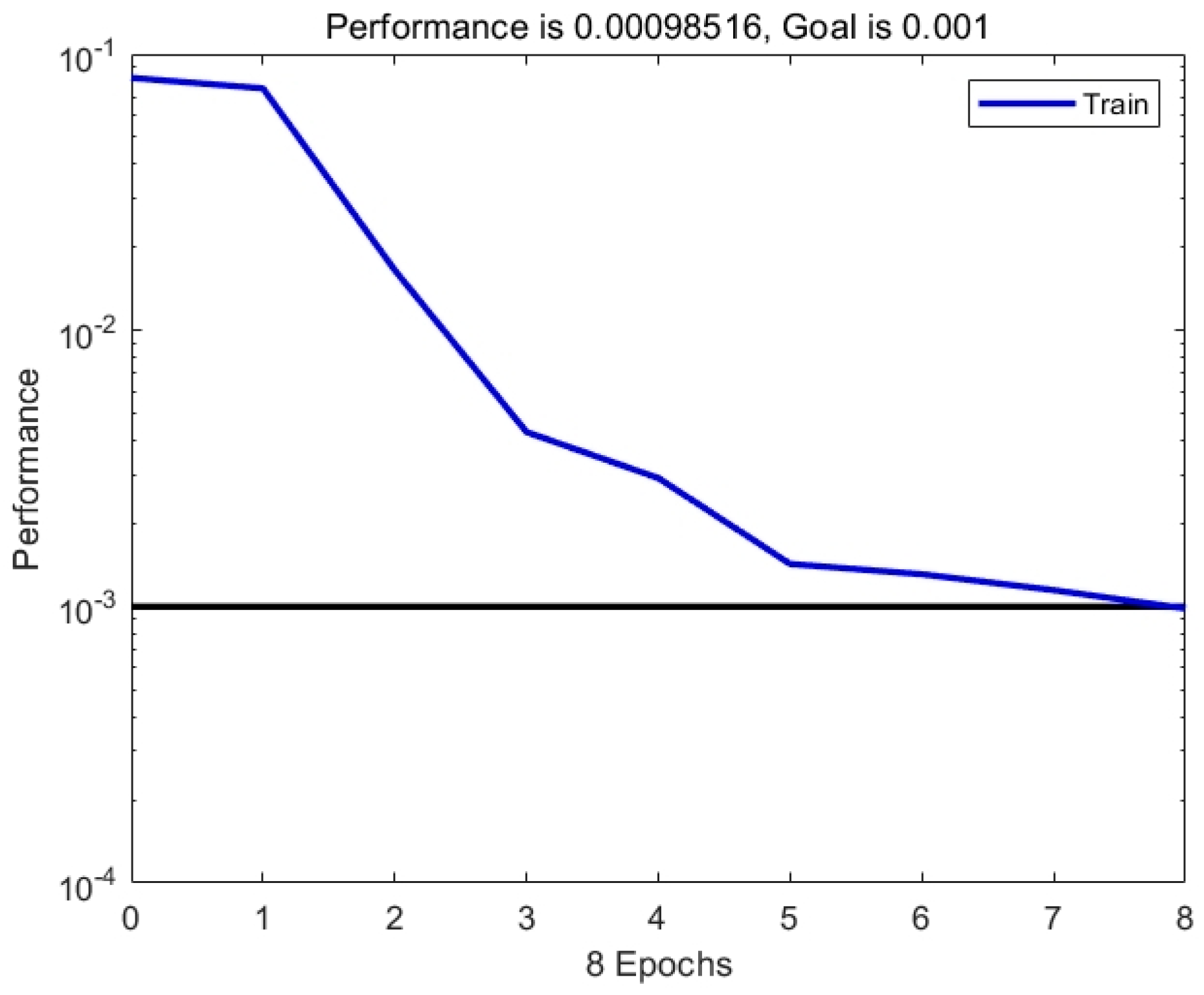
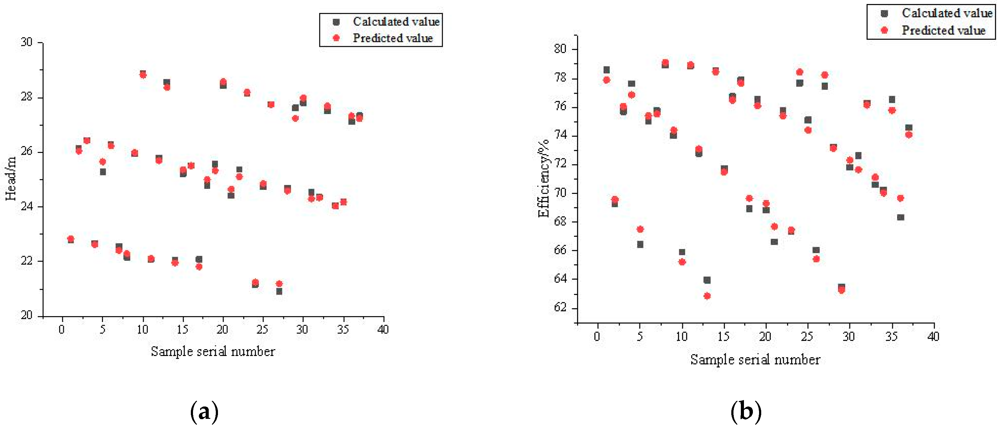
4.2. Hydraulic Performance Prediction Model

The approximate prediction model uses a small amount of sample data to establish an approximate function expression by interpolation or fitting mathematical methods, so as to carry out follow-up work such as prediction or optimization. The use of approximate predictive model methods can reduce the number of trials and improve the efficiency of optimization. Common approximate models include artificial neural networks, response surface methods, and Kriging models, among which artificial neural networks are widely used in various prediction-type problems with complex relationships because of their ability to adapt to complex non-linear relationships [24]. Therefore, in this paper, an artificial neural network is used to establish a hydraulic performance prediction model for submersible well pumps. As the research progresses, more than forty types of neural network models have been developed, among which BP neural networks and RBF neural networks are widely welcomed by researchers in various fields.

BP neural networks are relatively simple in structure, but they can easily be affected by local optimal solutions, and the learning efficiency of the network is fixed, which leads to a large amount of time required to reach convergence criteria. RBF neural networks have a strong generalization capability, good global approximation capability, are relatively unaffected by local optimal solutions, and have an efficient and simple structural form as well as the best approximation performance, so the training speed is faster [25]. Considering the above analysis, the RBF neural network is therefore used to create the prediction model.

In this paper, a three-factor, 37-level uniform experimental design was used [26]. Based on ANSYS CFX, 37 groups of models were simulated, and the results were used as training samples. According to the uniform test design table and its use table, the corresponding structural parameters are calculated according to the value range of the outlet placement angle β₂, the outlet width b₂, and the blade wrap angle φ, and then the corresponding head and efficiency are calculated based on the corresponding structural parameters. The results are shown in

Table 7. Numerical simulation results of external characteristics.

Sample Serial Number	Exit Placement Angle β2	Outlet Width b2	Blade Wrap Angle φ	Lift	Efficiency
1	17	9.8	102	22.8017	78.5818
2	17.5	12	74	26.1444	69.28
3	18	14.2	120	26.4369	75.7106
4	18.5	9	92	22.6546	77.6523
5	19	11.2	64	25.2747	66.4328
6	19.5	13.4	110	26.2874	75.0112
7	20	8.2	82	22.5566	75.7508
8	20.5	10.4	128	22.1592	78.9182
9	21	12.6	100	25.939	74.0439
10	21.5	14.8	72	28.869	65.9174
11	22	9.6	118	22.0847	78.8892
12	22.5	11.8	90	25.7813	72.795
13	23	14	62	28.5728	63.9778
14	23.5	8.8	108	22.055	78.5192
15	24	11	80	25.2196	71.7224
16	24.5	13.2	126	25.5187	76.7383
17	25	8	98	22.0859	77.8786
18	25.5	10.2	70	24.7811	68.9254
19	26	12.4	116	25.5758	76.5512
20	26.5	14.6	88	28.426	68.8344
21	27	9.4	60	24.4149	66.6407
22	27.5	11.6	106	25.3771	75.8033
23	28	13.8	78	28.1632	67.3917
24	28.5	8.6	124	21.1633	77.6949
25	29	10.8	96	24.7257	75.1141
26	29.5	13	68	27.7594	66.0542
27	30	7.8	114	20.9093	77.4695
28	30.5	10	86	24.6849	73.2271
29	31	12.2	58	27.6284	63.4781
30	31.5	14.4	104	27.8102	71.8061
31	32	9.2	76	24.5471	72.6405
32	32.5	11.4	122	24.3591	76.2711
33	33	13.6	94	27.5183	70.6124
34	33.5	8.4	66	24.0505	70.2596
35	34	10.6	112	24.1895	76.5615
36	34.5	12.8	84	27.1259	68.3395
37	35	15	130	27.3392	74.5881

.

In this study, MATLAB2018b software was used to write and simulate the RBF neural network program, using the newrb function to establish the network topology in the form shown in the following equation:

$$net=newrb(P,T,GOAL,SPREAD,MN,DF)$$

(13)

where P is the input matrix of order R × Q; T is the output matrix of order S × Q; GOAL is the mean square error target (default = 0); SPREAD is the expansion rate of the radial basis function (default = 1.0); MN is the maximum number of neurons (default Q); and DF is the number of neurons added between adjacent displays (default = 25). In this paper, GOAL is set to 0.001, SPREAD is set to 2, and all other default values are used. The training iteration process is shown in Figure 7. From the diagram, it can be seen that after the iteration to the eighth step, the error of 0.001 has been met and the training is complete.

To test the accuracy of the RBF neural network predictions, the sample data was re-entered into the network as test data for prediction, and the corresponding predicted head and predicted efficiency were obtained as shown in Figure 8. As can be seen from the graph, the difference between the CFX calculated values and the RBF neural network predictions is small, with a maximum error of 1.5% for the pump head and 1.9% for efficiency.

Three sets of structural parameters are randomly generated to predict and model simulation calculations, respectively, and then error analysis is carried out. The results are shown in

Table 8. Error analysis of numerical calculation results and prediction model results.

Serial Number	Exit Placement Angle β2	Outlet Width b2	Blade Wrap Angle φ	Lift		Error	Efficiency		Error
				Calculated Value	Predicted Value		Calculated Value	Predicted Value
1	17	10	102	23.3586	23.0377	−1.38%	76.9654	77.7294	0.99%
2	27.5	12.2	72	26.6137	26.8979	1.07%	66.8634	67.6188	1.13%
3	23	11	98	24.7361	24.601	−0.55%	74.3373	75.3969	1.43%

. The maximum error for the pump head is 1.38%, and the maximum error for efficiency is 1.43%, which is within the permissible range of engineering, so the RBF neural network prediction model can be considered feasible and can be used as an adaptation function model for the next multi-objective particle swarm optimization.

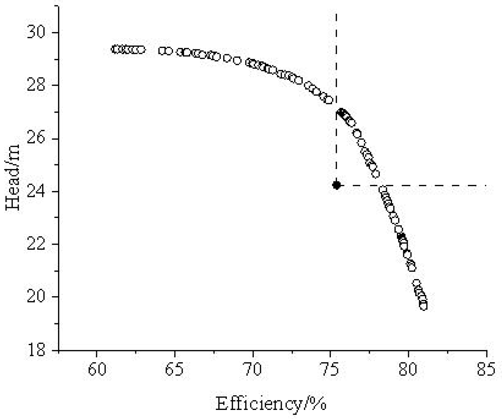
4.3. Multi-Objective Particle Swarm Optimization Algorithm Optimization

The particle swarm optimization continuously adjusts the particles’ own velocity towards the extreme value during the computational solution process without setting empirical parameters as in the genetic algorithm, and the better particle positions in the swarm algorithm are recorded. Compared with genetic algorithms, particle swarm optimization can converge faster in most cases [27]. Therefore, particle swarm optimization is chosen to solve the neural network prediction fitness function model in this paper.

The particle swarm optimization has two core formulas: the velocity formula and the position formula, as shown in the following equation:

$$V_i^d=\omega v_i^d+c_1{r}_1(p_i^d{x}_i^d)+c_2{r}_2(p_g^d-x_i^d)$$

(14)

$$X_i^d=x_i^d+v_i^d$$

(15)

where X_i = ($x_i^1$,$x_i^2$,…,$x_i^D$) is a solution in D-dimensional space; P_i = ($p_i^1$,$p_i^2$,…,$p_i^D$) is the position nearest to the optimum among all positions; P_g = ($p_g^1$,$p_g^2$,…,$p_g^D$) is the position nearest to the optimum among all positions through which all particles pass; V_i = ($v_i^1$,$v_i^2$,…,$v_i^D$) is the velocity of the particle; ω is the inertia weight; c₁, c₂ is the learning factor; and r₁, r₂ is any random number between 0 and 1.

In this paper, the multi-objective particle swarm optimization is used, based on the MATLAB software platform for programming simulation, and the sample results of the RBF neural network training are used as the fitness model for this optimization, with parameters set as follows: the number of particles is 100, the number of particle reserves is 100, the inertia weight is 0.7298, and both learning factors are 1.49445. After 500 iteration steps, the results are shown in Figure 9. It can be seen from the figure that the horizontal coordinate efficiency and the vertical coordinate lift have a mutually exclusive relationship, and the 100 Pareto optimal solutions obtained constitute a relatively smooth curve. The optimal solutions are also more evenly distributed, so the solution can be considered correct and reliable.

The edge points on both sides of the Pareto front are defined as the head optimum and the efficiency optimum resulting from the solution. The initial model is simulated by the CFD method. The optimal head individual is the model at the optimal head point predicted by the MOPSO algorithm. The optimal efficiency individual is the model at the optimum efficiency point as predicted by the MOPSO algorithm.

Table 9. Comparison of external characteristics before and after optimization.

Models	Lift (m)	Efficiency (%)
Initial model	24.2396	75.3835
Individuals with optimum head	29.3740	61.1736
Optimal efficiency individual	19.6603	80.9638

shows the comparison of the hydraulic performance of the submersible well pump before and after optimization. It can be seen from Table 9 that the head of the optimal individual is 5.1344 m higher than the initial model, but the efficiency is reduced by 14.2099 percentage points. The efficiency of the optimal individual is 4.5793 m lower than the initial model, but the efficiency is increased by 5.5803 percentage points.

If the head optimum and the efficiency optimum are chosen as the final optimization results, although there is an increase in the pump head and efficiency, there is also a significant decrease in efficiency and head. Therefore, two solutions are to be found on the Pareto front, denoted as head-optimal and efficiency-optimal, such that they each satisfy: (1) Under the condition that the efficiency is not reduced, the head is improved to the greatest extent; (2) The efficiency is improved to the greatest extent without reducing the head. It is easy to see that the two points are the horizontal and vertical coordinates of the initial model as indicators, and the intersection of these two lines with the Pareto front curve is the intersection of the vertical and horizontal lines, respectively. This is shown in Figure 10 below.

The Pareto solution at the boundary point within the right-angle intersection is defined as the better point. The higher-head individual is modeled by the structural parameters at the optimal head point and calculated by the CFD method of simulation. This individual is the model with the best head point predicted by the MOPSO algorithm. The higher-efficiency individual is modeled by the structural parameters at the optimal efficiency point and simulated by the CFD method. This individual is the model with the best efficiency point predicted by the MOPSO algorithm.

The structural parameters corresponding to the higher head and higher efficiency are modeled and simulated by CFD calculations according to the obtained higher head and higher efficiency, and the structural parameters are shown in

Table 10. Comparison of structural parameters before and after optimization.

Structural Parameters	Exit Placement Angle β2	Outlet Width b2	Blade Wrap Angle φ
Initial model	27	10	97
Individuals with better head	17	15	122
Individuals with better efficiency	17	13	130

. From the table, it can be seen that whether it is to increase the head or improve the efficiency, it is necessary to reduce the outlet angle and increase the outlet width and blade wrap angle.

The individuals with the best head or best efficiency were compared with the head and efficiency of the initial model, as shown in

Table 11. Comparison of external characteristics before and after optimization.

Models	Lift (m)	Efficiency (%)
Initial model	24.2396	75.3835
Individuals with better head	26.8926	74.7845
Individuals with better efficiency	24.8755	77.6431

. From the table, it can be seen that the selected individuals with the best head or best efficiency satisfy the maximum increase in head without a decrease in efficiency and the maximum increase in efficiency without a decrease in head, respectively. The individual with the best head has an increase of 2.653 m compared to the initial model head and a decrease of about 0.6 percentage points in efficiency, which is a small and acceptable decrease in efficiency. The individual with the best efficiency has an increase of about 0.6 m compared to the initial model head and an increase of about 2.3 percentage points in efficiency.

5. Analysis of Results

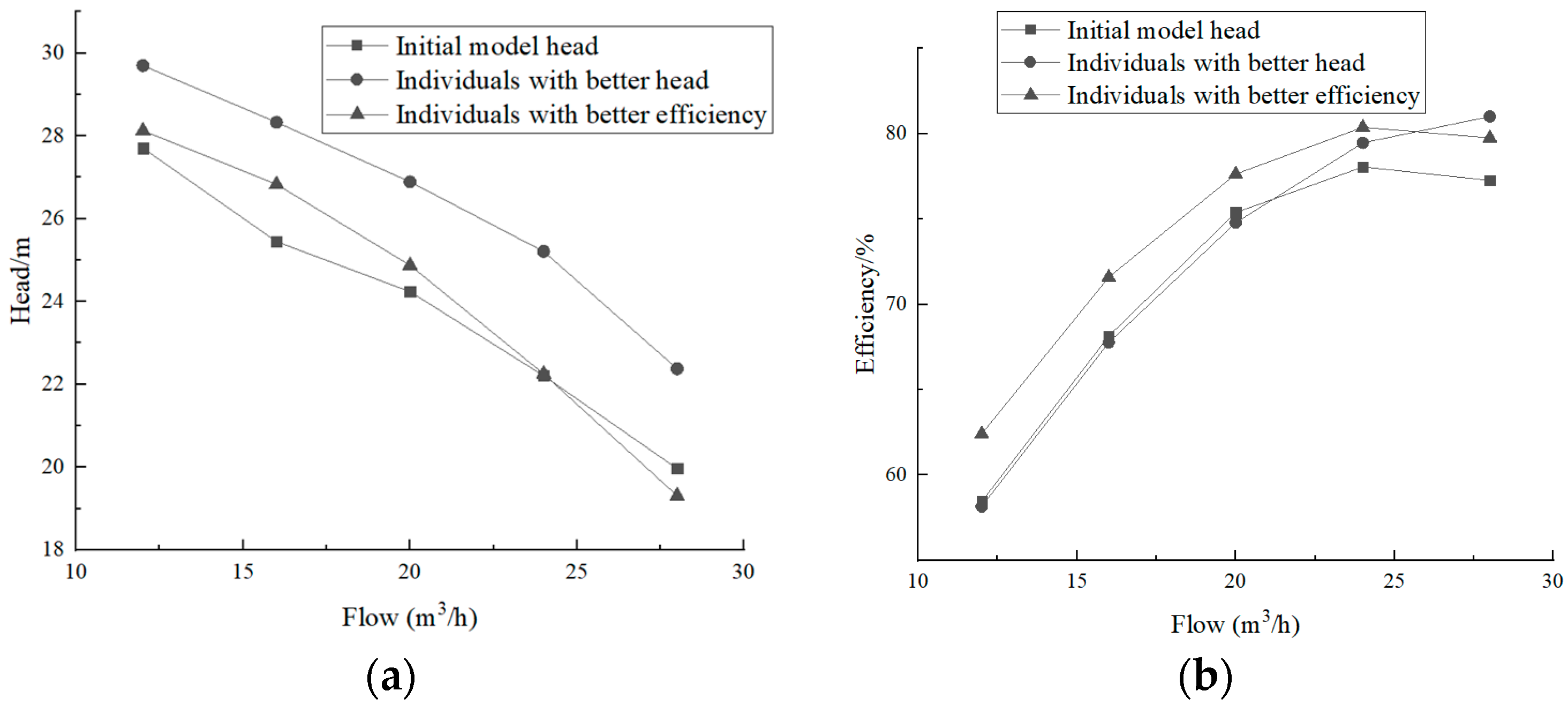
5.1. External Characterization

The five working conditions of the initial model, the individual with a better head and the individual with better efficiency from 0.6 times to 1.4 times of the standard condition, are simulated, respectively, and the external characteristics before and after optimization are shown in Figure 11. It can be seen from the diagram that under standard working conditions, the head of the individual with a better head reaches about 26.9 m. At low flow rates or at standard flow rates, the heads of the higher-efficiency individuals are higher than those of the initial model, but at 1.2 times the standard operating conditions, the heads of the higher-efficiency individuals are similar to those of the initial model. The efficiency of the better individual was improved at the low flow rate, the standard operating conditions, and the 1.2 times standard operating conditions, and only at the 1.4 times standard operating conditions was the efficiency of the better individual slightly lower than the efficiency of the higher-head individual, and at the standard operating conditions, the efficiency of the better individual reached 77.64%. The efficiency of the higher-head individual was comparable to the initial model at both low flow and standard conditions but was higher than the initial model at high flow conditions. In order to further investigate the internal causes of the external characteristics, a pressure and velocity flowline analysis is carried out using the secondary impeller at standard operating conditions and the secondary space guide vane as an example.

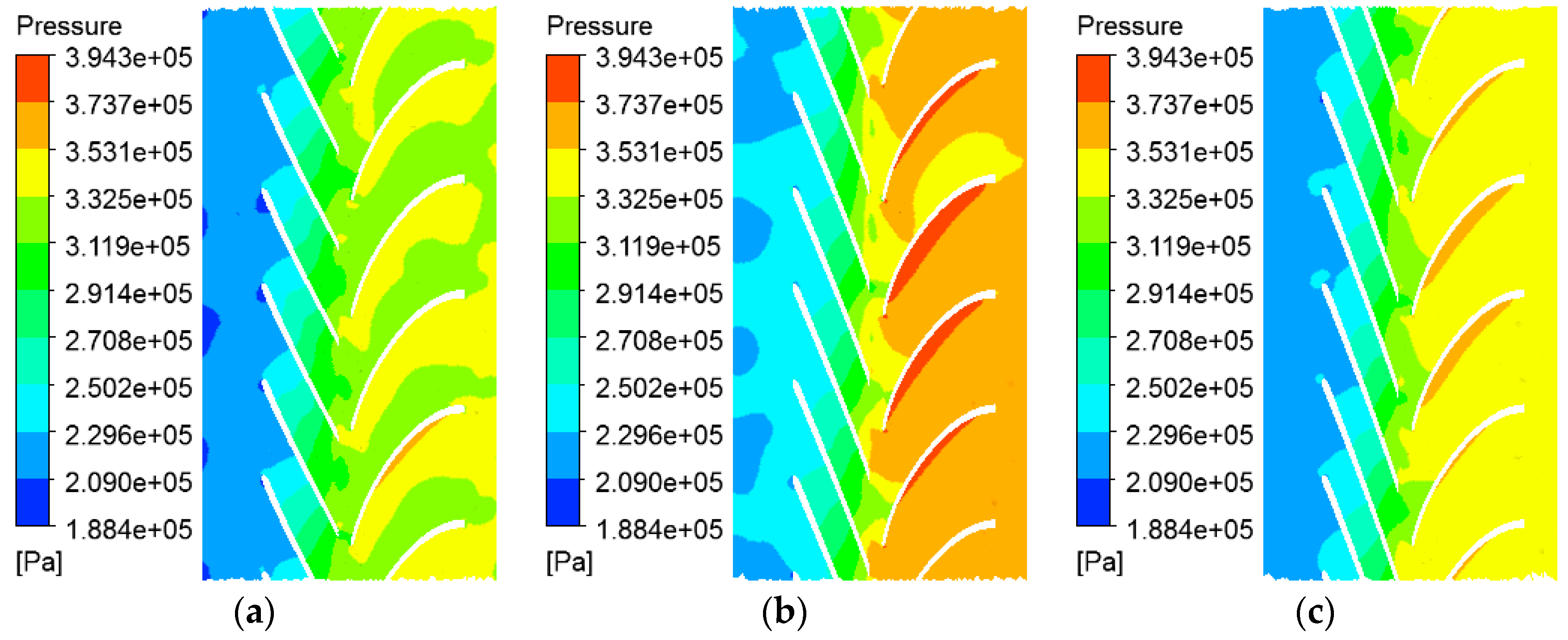
5.2. Pressure Distribution Analysis

Figure 12 shows the pressure expansion distribution cloud diagram of the middle section of the secondary impeller and the secondary space guide vane before and after optimization. The pressure in the impeller inlet area is the lowest, with a minimum static pressure of 188.4 KPa, and the pressure in the impeller flow path to the impeller outlet area gradually increases due to the work performed by the impeller rotation and flows through the space guide vane to reach a maximum static pressure of 394.3 KPa. In the impeller inlet area, the low pressure area of the higher-head individual is reduced compared to that of the initial model and is only distributed in a block shape near the blade inlet. The impeller inlet area of the more efficient individual has a more uniform low-pressure area than the initial model. Compared to the initial model, the impeller work capacity of the higher-head and higher-efficiency individuals is significantly increased, and the pressure gradient in the impeller flow path is more obvious, with the most obvious pressure gradient distribution for the higher-head individual and the second most obvious for the higher-efficiency individual. In the area of the spatial guide vane, the working surface of the guide vane is facing the incoming media conveyed by the impeller, and the impulse causes a strip of high pressure to be generated close to the working surface. The pressure distribution in the spatial guide vane area is more uniform for the higher-head and higher-efficiency individuals than in the initial model, and the pressure values in the spatial guide vane area are highest for the higher-head individual. The yellow area of the spatial guide vane of the more efficient individual is significantly larger than the yellow area of the spatial guide vane of the initial model, which is one of the fundamental reasons why the head of the more efficient individual does not decrease. The yellow area of the spatial guide vane of the more efficient individual is significantly more uniform than the yellow area of the spatial guide vane of the initial model, which is also one of the fundamental reasons for the increased efficiency of the more efficient individual.

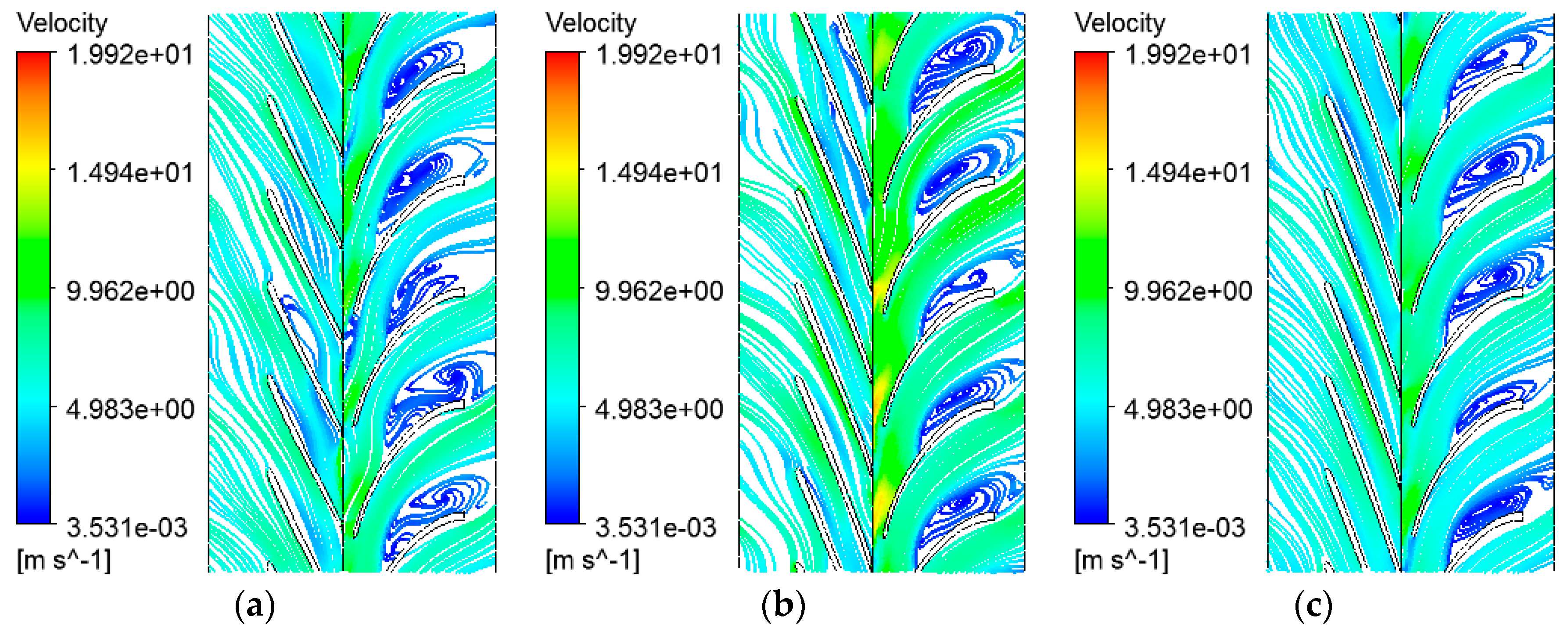
5.3. Velocity Flow Line Analysis

Figure 13 is the distribution map of the middle section velocity streamline of the secondary impeller and the secondary space guide vane before and after optimization. In the impeller inlet area, the initial model, the higher-head individual, and the higher-efficiency individual all show varying degrees of divergence, with the higher-head individual showing the most severe divergence, followed by the initial model, and the higher-efficiency individual showing a more uniform and smooth flow line. Each impeller blade has a small part of the low speed zone close to the working surface, which results in a pressure difference between the impeller blade and the working surface at the corresponding position. In the spatial guide vane area, the guide vane working surface diverts the impeller conveying medium, the flow line is uniform, and the direction is consistent with the direction of the guide vane blade. Due to the media off-flow, the back of the guide vane blade forms a vortex area to varying degrees. Compared to the initial model, the vortex area of the individual with the better head and the individual with the better efficiency is relatively small, and the vortex area flow line is relatively more regular.

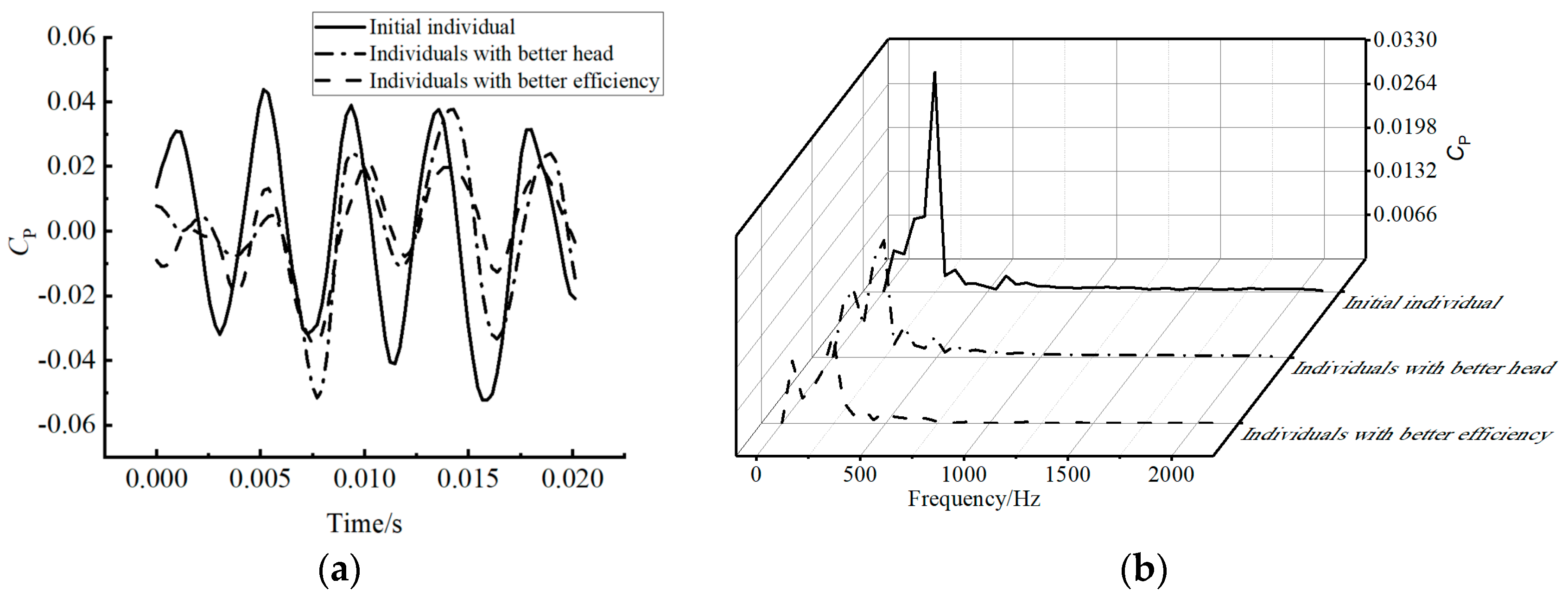
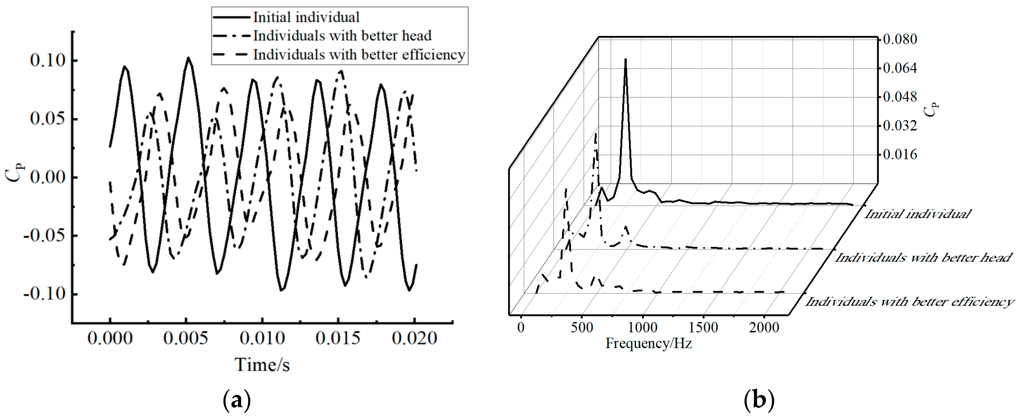
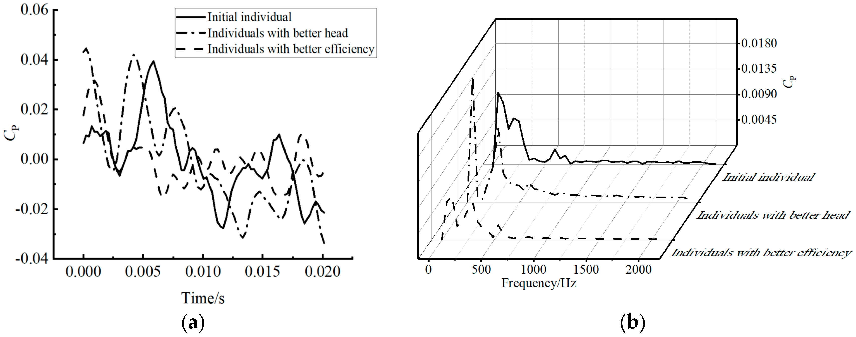
5.4. Pressure Pulsation Analysis

Figure 14 shows the pressure pulsation characteristics at the Y1 monitoring point set at the secondary impeller inlet for the three models before and after optimization. Figure 14a shows the time domain distribution of the pressure pulsation at point Y1. Due to the strong dynamic and static interference effects, five wave peaks appear in one cycle, which are equal to the number of guide vanes. The peaks and troughs of the time domain characteristics of the pressure pulsation for the three models before and after optimization correspond to each other, which indicates that the optimization has not affected the phase values of the pressure pulsation.

Figure 14b shows the frequency domain distribution of pressure pulsation at the Y1 monitoring point. The dominant frequency of pressure pulsation before and after optimization is around the doubled guide vane frequency, so the dynamic interference effect is dominant. After optimization, the magnitude of pressure pulsation at the inlet of the secondary impeller is significantly lower for the individual with the better head and the individual with the better efficiency. The pressure pulsation of the individual with the better head was reduced by 46.7% compared to the initial individual, and the pressure pulsation of the individual with the better efficiency was reduced by 59.9% compared to the initial individual.

Figure 15 shows the pressure pulsation characteristics at the Y2 monitoring point at the outlet of the secondary impeller for the initial individual model before optimization, the individual model with the better head after optimization, and the individual model with the better efficiency after optimization. Compared with Figure 14a, there are still five peaks in the individual models before and after optimization. The difference is that the fluctuation of the pressure pulsation coefficient in Figure 15a is significantly larger, which is the result of the work performed by the impeller rotation. The peak position of the more efficient individual corresponds to the trough position of the initial individual, while the phase of the higher-head individual is in between, which indicates that the phase value of the pressure pulsation at the outlet of the secondary impeller has changed after optimization.

As can be seen from the frequency domain characteristics plot in Figure 15b, the dominant frequency of pressure pulsation before and after optimization is still around the doubled guide vane frequency, which indicates that dynamic interference is still the dominant influencing factor. After optimization, the pressure pulsation amplitude of the individual with the better head is reduced by 21.3% compared to the initial individual, and the pressure pulsation amplitude of the individual with the better efficiency is reduced by 29% compared to the initial individual.

Figure 16 shows the pressure pulsation characteristics at monitoring point Y3 at the inlet of the secondary space guide vane for the initial individual model before optimization, the individual model with the better head after optimization, and the individual model with the better efficiency after optimization. As can be seen in Figure 16a, the number of pressure fluctuations at this point becomes six before and after optimization, the same as the number of impeller blades, again due to strong dynamic interference effects. The peak and trough positions of the more efficient individual correspond essentially to those of the initial individual, with the phase of the higher-head individual remaining in between. This indicates that the optimization has changed the phase value of the pressure pulsation at the inlet of the secondary space guide vane.

As can be seen in Figure 16b, the dominant frequency of pressure pulsation before and after optimization is around the doubled impeller blade frequency. The optimized individual with the better head has a 20.2% reduction in pressure pulsation amplitude compared to the initial individual, and the individual with the better efficiency has a 30.2% reduction in pressure pulsation amplitude compared to the initial individual.

Figure 17 shows the pressure pulsation characteristics at monitoring point Y4 at the outlet of the secondary spatial guide vane for the three models before and after optimization. In Figure 17a, the pressure pulsation amplitude at this monitoring point is significantly reduced compared to the pressure pulsation amplitude at the inlet of the space guide vane, which is due to the weakening of the pressure pulsation amplitude after the fluid is guided through the space guide vane. The regularity of the pressure pulsation at this point is significantly reduced by the effect of multiple dynamic interference couplings.

As can be seen in Figure 17b, the pressure pulsation amplitude reaches a maximum around doubling the shaft frequency, which is due to the fact that at the guide vane outlet, the effect of dynamic interference is weaker and the influence of the shaft frequency dominates. The pressure pulsation amplitude of the optimized individual with the better head increased by 75.9% compared to the initial individual, while the pressure pulsation amplitude of the individual with the better efficiency decreased by 46.5% compared to the initial individual. The increase in pressure pulsation for the higher-head individual compared to the pre-optimized individual is probably due to the influence of multiple dynamic and static interference couplings at the guide vane outlet and the higher static pressure energy at the guide vane outlet for the higher-head individual, which is more strongly influenced by the dynamic and static interference coupling. The pressure pulsation coefficient for the higher-head individual is approximately 0.02, which is still relatively small compared to the other locations and is within acceptable limits.

6. Conclusions

(1)

Based on the Plackett-Burman experimental design in the professional experimental design software Design Expert 12.0, it was determined that the impeller outlet settling angle, outlet width, and blade wrap angle were significant influencing factors. The difference between the predicted value of the RBF neural network and the calculated value of the CFX was small, and the maximum error of its head was 1.5% and the maximum error of its efficiency was 1.9%, i.e., the RBF neural network prediction model is accurate and reliable.

(2)

In this study, the pump performance prediction model of the RBF neural network and the optimization design method of the multi-objective particle swarm optimization algorithm are adopted. These improvements enable the research to better fit complex pump performance models and perform design optimizations considering multiple optimization objectives. In the optimization process, the search strategy is adjusted in time to avoid being affected by the local optimal solution. The algorithm can better explore the design space and find the global optimal solution, thereby improving the stability and accuracy of the optimization results. Finally, the optimal outlet angle, outlet width, and blade wrap angle of the individuals with better head and efficiency were determined to be 17°, 15 mm, 122°, and 17°, 13 mm, 130°, respectively.

(3)

The optimized head has increased by approximately 2.65 meters compared to the head of the superior individual, and the efficiency has increased by approximately 2.3 percentage points compared to the efficiency of the superior individual. The pressure gradient in the impeller flow path is more pronounced after optimization, the work capacity is significantly improved, the spatial guide vortex area is smaller, and the flow line is more regular. Compared to the initial individual model, the pressure pulsation in the impeller inlet and outlet and the spatial guide vane inlet of the higher-head individual is reduced by 46.7%, 21.3%, and 20.2%, respectively, while the pressure pulsation in the spatial guide vane outlet increases by 75.9%, but the pressure pulsation coefficient after the increase is still small and within the acceptable range. The higher-efficiency individual had a 59.9%, 29%, 30.2%, and 46.5% reduction in pressure pulsation amplitude at the impeller inlet and outlet as well as at the space guide vane inlet and outlet, respectively.

References

1. Zhang, X.Y.; Jiang, C.X.; Lv, S.; Wang, X.; Li, W.-Y. Clocking effect of outlet RGVs on hydrodynamic characteristics in a centrifugal pump with an inlet inducer by CFD method. Eng. Appl. Comput. Fluid Mech. 2021, 15, 222–235. [Google Scholar] [CrossRef]
2. Lai, F.; Zhu, X.; Duan, Y.; Li, G. Clocking effect in a centrifugal pump with a vaned diffuser. Mod. Phys. Lett. B 2020, 34, 205–286. [Google Scholar] [CrossRef]
3. Tan, M.; Lian, Y.; Wu, X.; Liu, H. Numerical investigation of clocking effect of impellerson a multistage pump. Eng. Comput. 2019, 10, 150–158. [Google Scholar]
4. Gu, Y.; Pei, J.; Yuan, S.; Wang, W.; Zhang, F.; Wang, P.; Appiah, D.; Liu, Y. Clocking effect of vaned diffuser on hydraulic performance of high-power pump by using the numerical flow loss visualization method. Energy 2019, 170, 986–997. [Google Scholar] [CrossRef]
5. Yuan, S.Q.; Wang, W.J.; Pei, J.; Zhang, J.F.; Mao, J.Y. Multi-objective optimization of low-specific-speed centrifugal pump. J. Agric. Eng. 2015, 31, 46–52. [Google Scholar]
6. Li, M.C. Research on Automatic Optimization Design of Mixed-Flow Pump Impeller Based on Multi-Objective; Xihua University: Chengdu, China, 2015. [Google Scholar]
7. Wang, C.L.; Ye, J.; Zeng, C.; Xia, Y.; Luo, B. Multi-objective optimum design of high specific speed mixed-flow pump based on NSGA-IIgenetic algorithm. J. Agric. Eng. 2015, 31, 100–106. [Google Scholar]
8. Zhao, W.G.; Sheng, J.P.; Yang, J.H.; Song, Q.C. Optimization design and experiment of centrifugal pump based on CFD. J. Agric. Eng. 2015, 31, 125–131. [Google Scholar]
9. Liao, F.; Zhang, H. Optimization design of lower speed pump based on genetic algorithm. China Agric. Chem. News 2016, 37, 233–236. [Google Scholar]
10. Jiang, W.Z.; Duan, S.Q.; Yang, C.M.; Wang, G.C. Optimal design of centrifugal pump impeller based on CFD simulations and BP neural network. Mach. Tool Hydraul. 2016, 44, 67–70. [Google Scholar]
11. Wang, C.L.; Feng, Y.M.; Ye, J.; Luo, B.; Liu, K.K. Multi-objective parameters optimization of centrifugal slurry pump based on RBF neural network and NSGA-IIgenetic algorithm. J. Agric. Eng. 2017, 33, 109–115. [Google Scholar]
12. Tao, R.; Xiao, R.F.; Yang, W. Optimization design for axial fiow pump based on genetic algorithm. J. Irrig. Drain. Mach. Eng. 2018, 36, 573–579. [Google Scholar]
13. Li, Q.M.; Jiang, J.X.; Li, Y. Fuel pump impeller optimization design based on multi-object genetic algorithm. Mod. Manuf. Eng. 2018, 7, 121–126. [Google Scholar]
14. Wang, C.L.; Hu, B.B.; Feng, Y.M.; Li, K.K. Multi-objective optimization of double vane pum-p based on radial basis neural network and particle swarm. J. Agric. Eng. 2019, 35, 25–32. [Google Scholar]
15. Dong, M.; Yang, H.; Chen, T.Z. Multi-objective optimization design and numerical simulate-on of centrifugal pumps. China Rural. Water Hydropower 2019, 4, 154–157+161. [Google Scholar]
16. Ye, X.D.; Li, H.; Ma, Q.Y.; Han, Q.B.; Sun, X.L. Optimal Design of Vortex Pump Using Approximate Model and the Non-dominated Sorting Genetic Algorithm. J. Irrig. Drain. 2019, 38, 76–83. [Google Scholar]
17. Tong, Z.M.; Chen, Y.; Tong, S.G.; Yu, Y.; Li, J.F.; Hao, G.S. Multi-objective optimization design of low specific speed centrifugal pumps based on NSGA-III algorithm. China Mech. Eng. 2020, 31, 2239–2246. [Google Scholar]
18. Jiang, B.X.; Yang, J.H.; Bai, X.B.; Wang, X.H. Optimization of centrifugal pump blade based on high-dimensional hybrid model and genetic algorithm. J. Huazhong Univ. Sci. Technol. (Nat. Sci. Ed.) 2020, 48, 128–132. [Google Scholar]
19. Hao, Z.R.; Li, C.; Ren, W.L.; Wang, Y.; Hua, Z.L.; Liu, G. Optimization design of water jet pro-pulsion pump blade based on improved PSO algorithm. J. Irrig. Drain. Mach. Eng. 2020, 38, 566–570. [Google Scholar]
20. Wang, M.C.; Yuan, J.P.; Li, Y.J.; Zheng, Y.H. Multi-objective optimization of mixed-flow pu-mp impeller based on 3-D inverse design. J. Harbin Eng. Univ. 2020, 41, 1854–1860. [Google Scholar]
21. Siddique, M.H.; Afzal, A.; Samad, A. Design optimization of the centrifugal pumps via low fidelity models. Math. Probl. Eng. 2018, 2018, 3987594. [Google Scholar] [CrossRef]
22. Alawadhi, K.; Alzuwayer, B.; Mohammad, T.A.; Buhemdi, M.H. Design and optimization of a centrifugal pump for slurry transport using the response surface method. Machines 2021, 9, 60. [Google Scholar] [CrossRef]
23. Kim, J.H.; Oh, K.T.; Pyun, K.B.; Kim, C.K.; Choi, Y.S.; Yoon, J.Y. Design optimization of a centrifugal pump impeller and volute using computational fluid dynamics. IOP Conf. Ser. Earth Environ. Sci. 2012, 15, 032025. [Google Scholar] [CrossRef]
24. Pei, J.; Wang, W.J.; Yuan, S.Q. Advanced Optimization Theory and Technology for Vane Pu-Mps; Science Press: Beijing, China, 2019. [Google Scholar]
25. Ye, J.; Ge, L.D.; Wu, Y.X. An optimized RBF neural network for modulation recognition. J. Autom. 2007, 48, 652–654. [Google Scholar]
26. Fang, K.T. A method for determining the dominance of factors in orthogonal tests with varying numbers of levels. Math. Pract. Aware. 1978, 01, 33–36. [Google Scholar]
27. Wang, F.; Wang, X.J.; Sun, S.L. A reinforcement learning level-based particle swarm optimization algorithm for large-scale optimization. Inf. Sci. 2022, 602, 298–312. [Google Scholar] [CrossRef]
Figure 1. Computational domain assembly model.
Applsci 13 08772 g001
Figure 2. Meshing of the whole model.
Applsci 13 08772 g002
Figure 3. Boundary layer mesh refinement.
Applsci 13 08772 g003
Figure 4. Layout of monitoring points. (a) Impeller; (b) space guide leaf.
Applsci 13 08772 g004
Figure 5. Pump performance test schematic diagram.
Applsci 13 08772 g005
Figure 6. Comparison of pump performance test results with numerical simulation results.
Applsci 13 08772 g006
Figure 7. Iterative diagram of neural network training.
Applsci 13 08772 g007
Figure 8. External characteristic prediction error. (a) Lift; (b) efficiency.
Applsci 13 08772 g008
Figure 9. Pareto frontier distribution.
Applsci 13 08772 g009
Figure 10. Pareto frontier distribution truncation.
Applsci 13 08772 g010
Figure 11. Comparison of external characteristics before and after optimization. (a) Head; (b) efficiency.
Applsci 13 08772 g011
Figure 12. Cloud diagram of pressure expansion distribution in the middle section of the secondary impeller and secondary space guide vane before and after optimization. (a) Initial model; (b) individuals with better heads; (c) more efficient individuals.
Applsci 13 08772 g012
Figure 13. Unfold diagram of the velocity streamline in the middle section of the secondary impeller and secondary space guide vane before and after optimization. (a) Initial model; (b) individuals with better heads; (c) more efficient individuals.
Applsci 13 08772 g013
Figure 14. Pressure fluctuation characteristic diagram of the Y1 monitoring point before and after optimization. (a) Time domain; (b) frequency domain.
Applsci 13 08772 g014
Figure 15. Pressure fluctuation characteristic diagram of the Y2 monitoring point before and after optimization. (a) Time domain; (b) frequency domain.
Applsci 13 08772 g015
Figure 16. Pressure fluctuation characteristic diagram of the Y3 monitoring point before and after optimization. (a) Time domain; (b) frequency domain.
Applsci 13 08772 g016
Figure 17. Pressure fluctuation characteristic diagram of the Y4 monitoring point before and after optimization. (a) Time domain; (b) frequency domain.
Applsci 13 08772 g017