
Research on Process Quality Prediction and Control of Spindle Housings in Flexible Production Lines

Abstract
:1. Introduction
- (1)
- A fuzzy hierarchical analysis model is established for spindle housing. The index value of each scheme is analyzed and calculated, and a comprehensive analysis of various factors affecting the production line is conducted to determine the most excellent scheme for quality control.
- (2)
- A dynamic prediction model through the GM(1,1) principle is established to obtain sample prediction values, to train the residuals of the prediction values through a BP neural network for the network model, and to verify the validity and feasibility of the combined prediction scheme by analyzing and comparing the prediction value errors of the process quality data.
- (3)
- SPC control of the critical processes of a spindle box is used to achieve quality prediction and monitoring of each process in the production line, to complete the process quality prediction and control scheme for the flexible production line of a spindle box.
2. Flexible Production Line for Spindle Housing
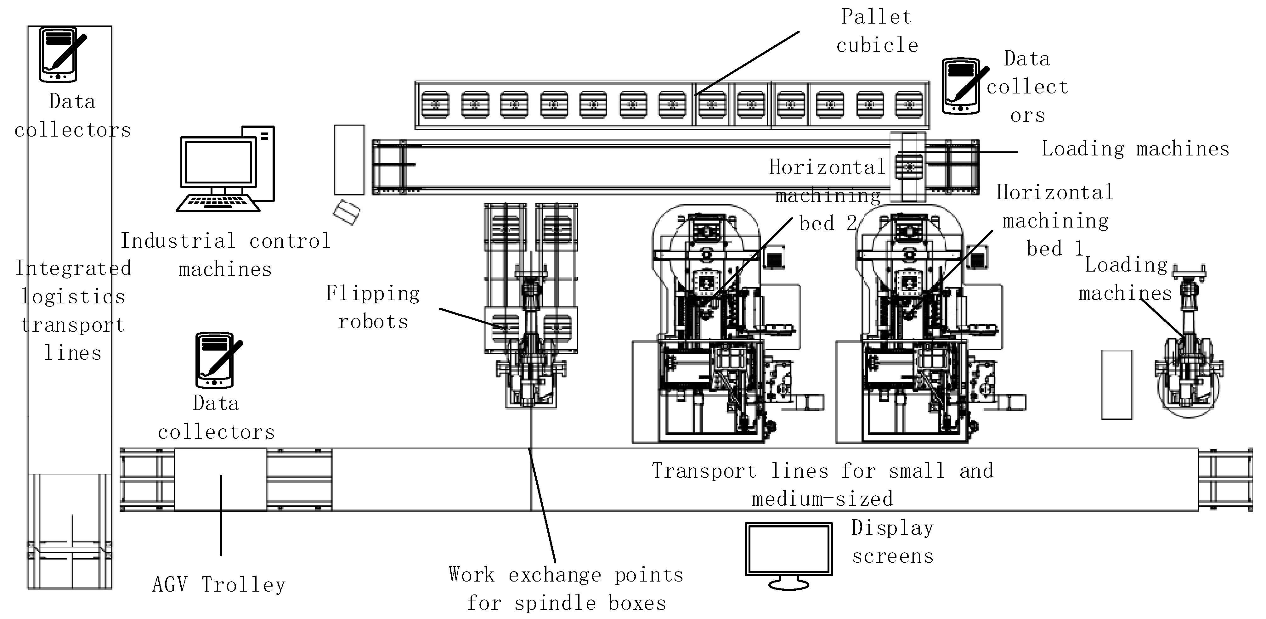
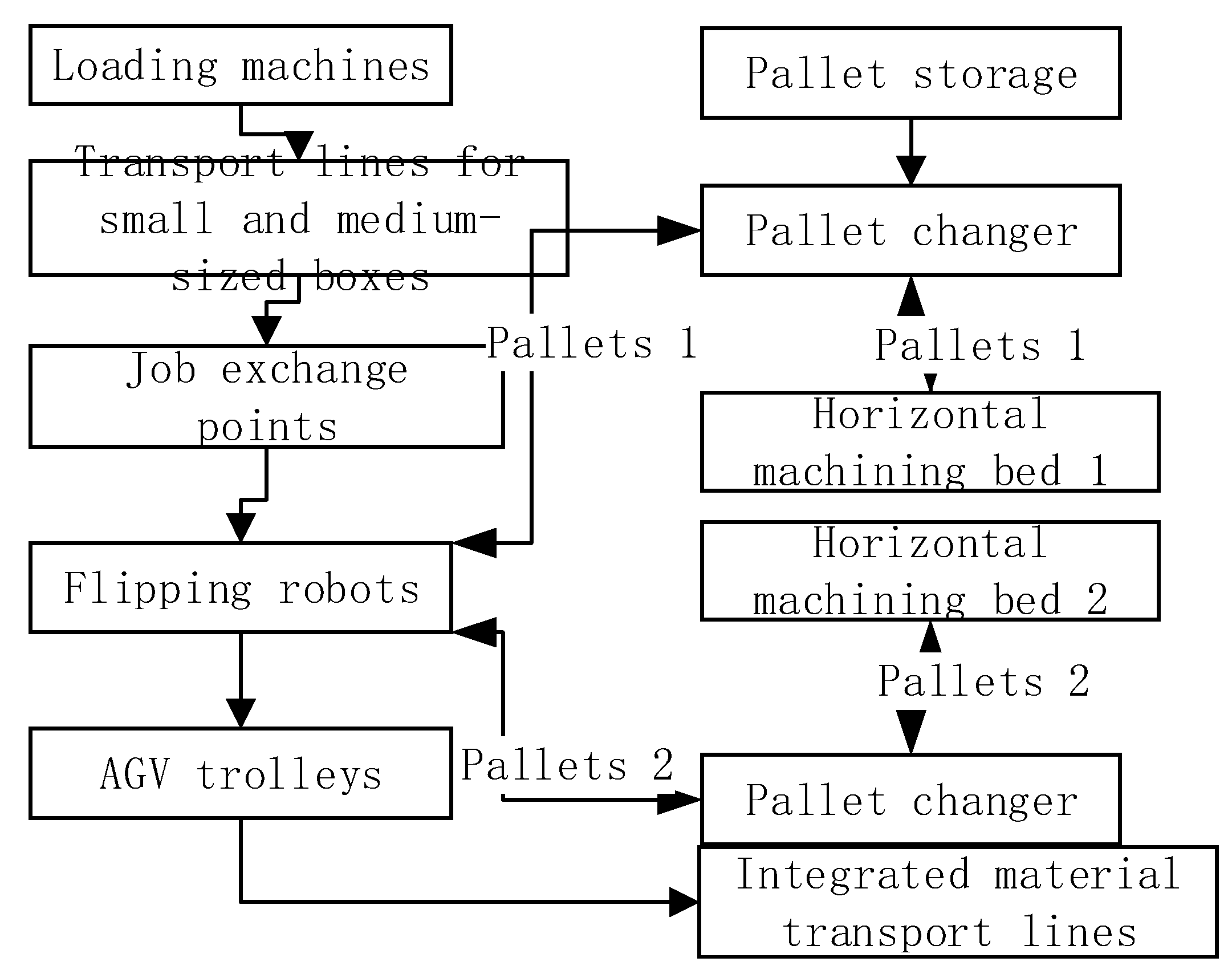
2.1. Introduction of the Spindle Box Flexible Production Line
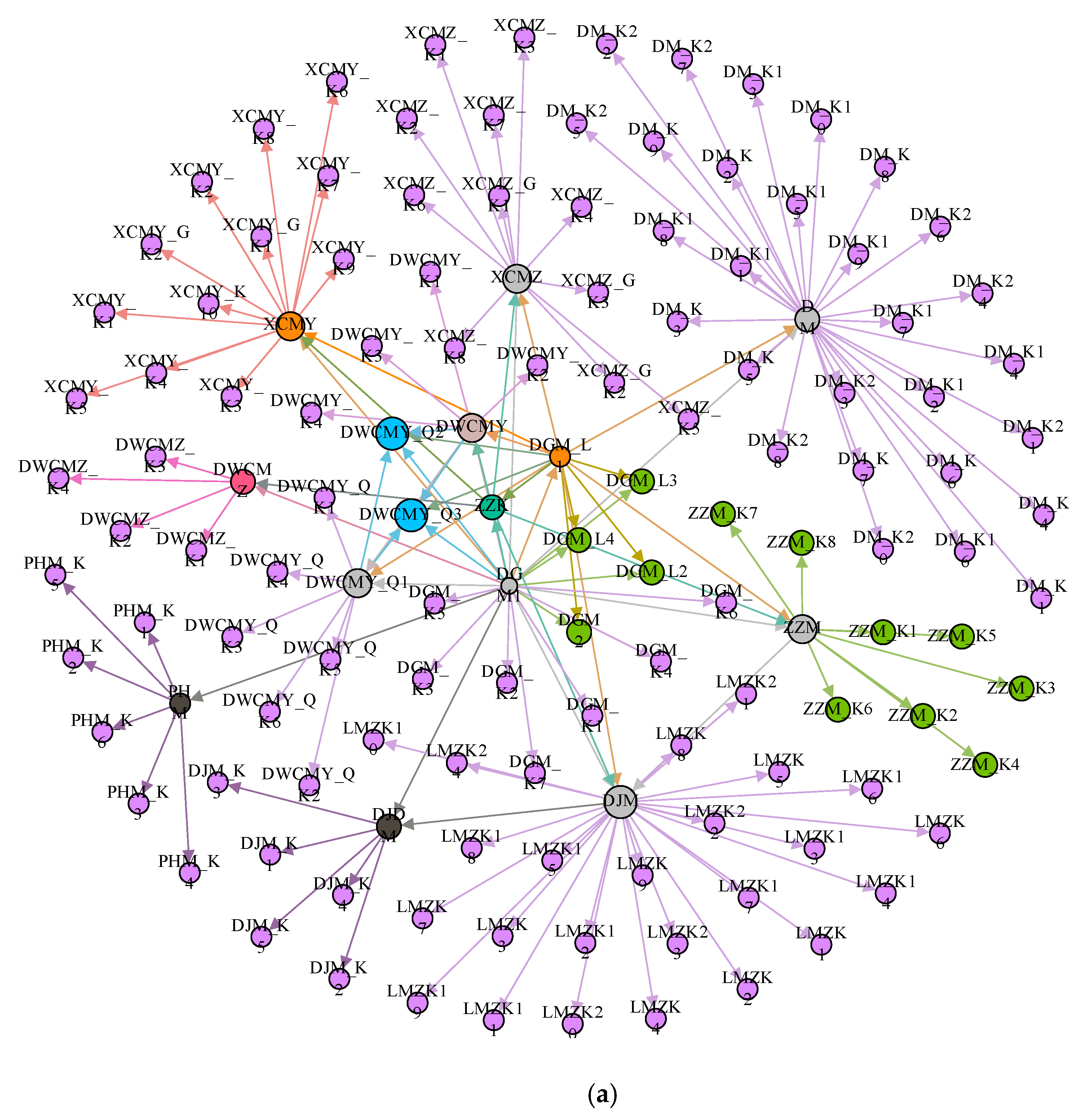
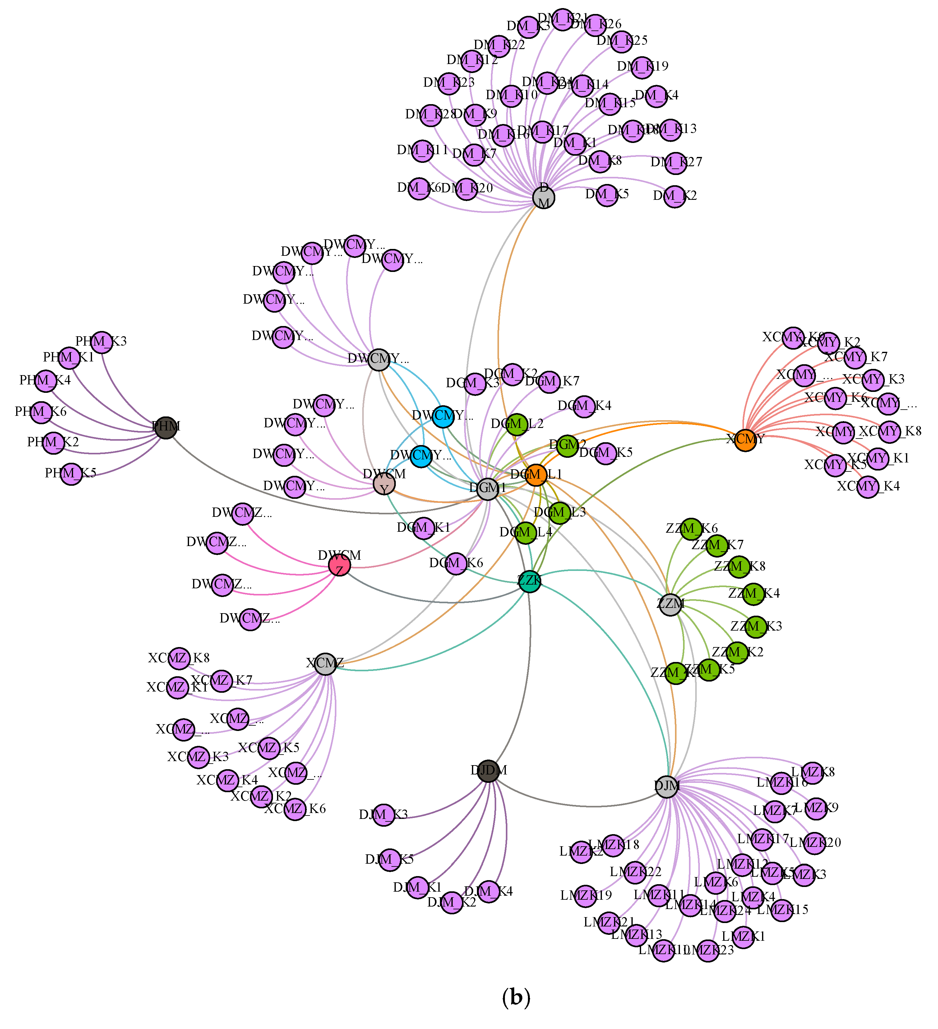
2.2. Spindle Housing Critical Process Machining Features Model
3. Influence Factor Analysis Model Based on Fuzzy Hierarchy Analysis
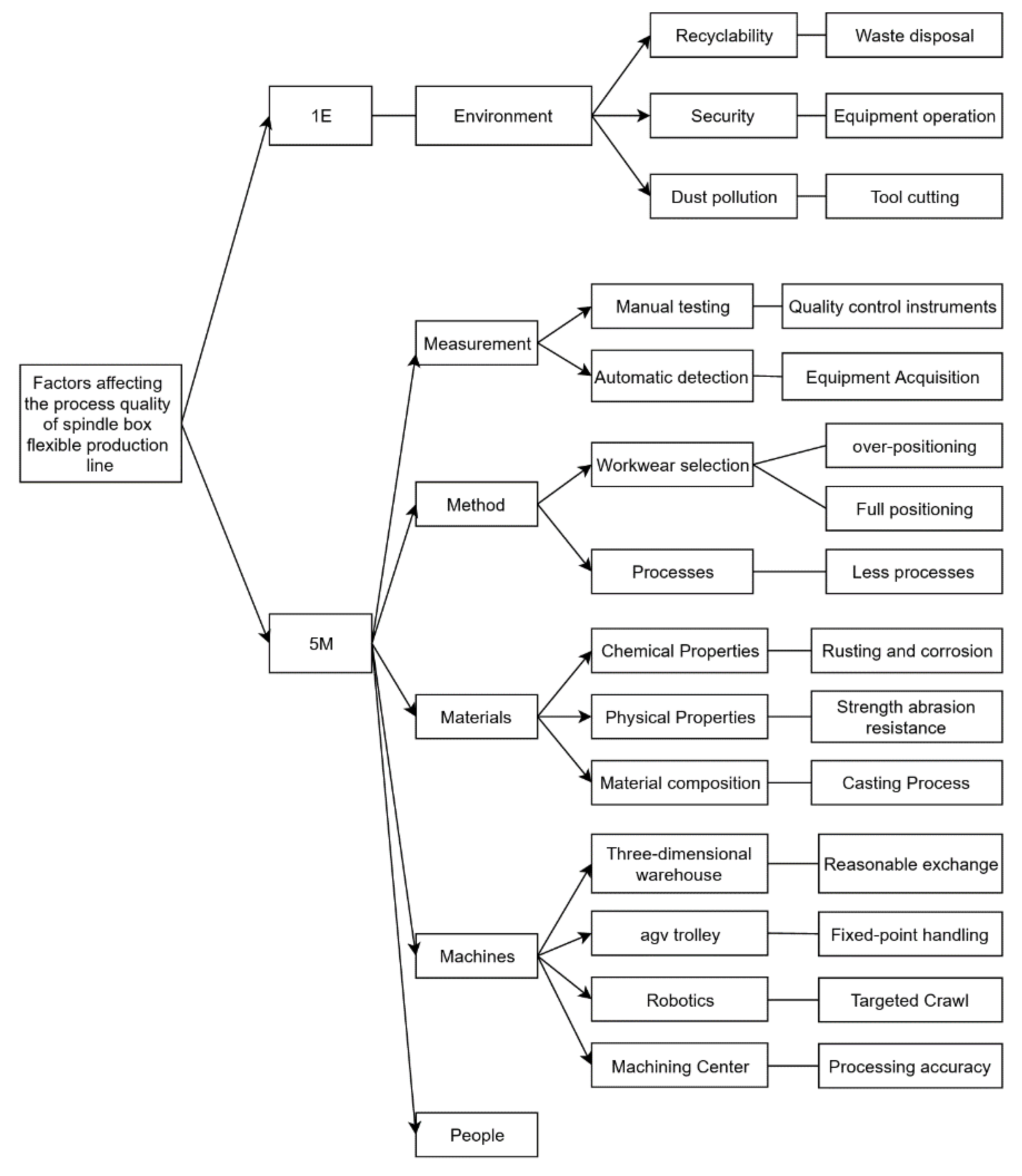
3.1. Analysis of Process Quality Influence Factors Based on 5M1E
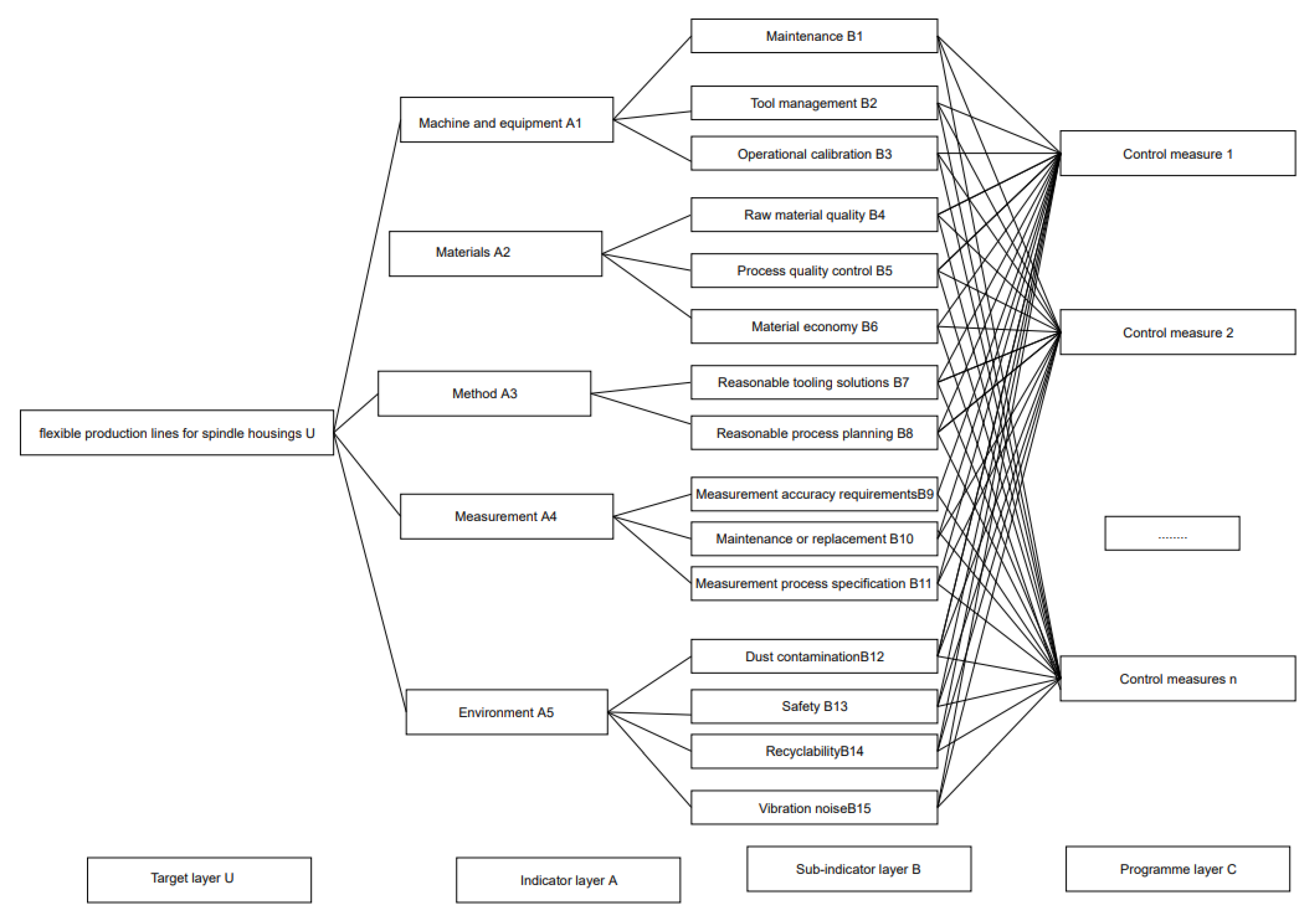
3.2. Process Quality Impact Factor Analysis Model
- (1)
- Establishment of the index optimization system
- (2)
- Establishment of the fuzzy complementary judgment matrix
3.3. Decision Analysis of Process Quality Influencing Factors
3.3.1. Index Layer Weights
3.3.2. Determination of Subindex Layer Weights
3.3.3. Hierarchical Total Ranking
3.3.4. Process Quality Control Scheme
4. Optimization of Critical Process Quality Prediction Control Based on GM(1,1)-BP
4.1. Process Quality Eigenvalue Prediction Model
4.1.1. Improved Dynamic GM(1,1) Prediction Model
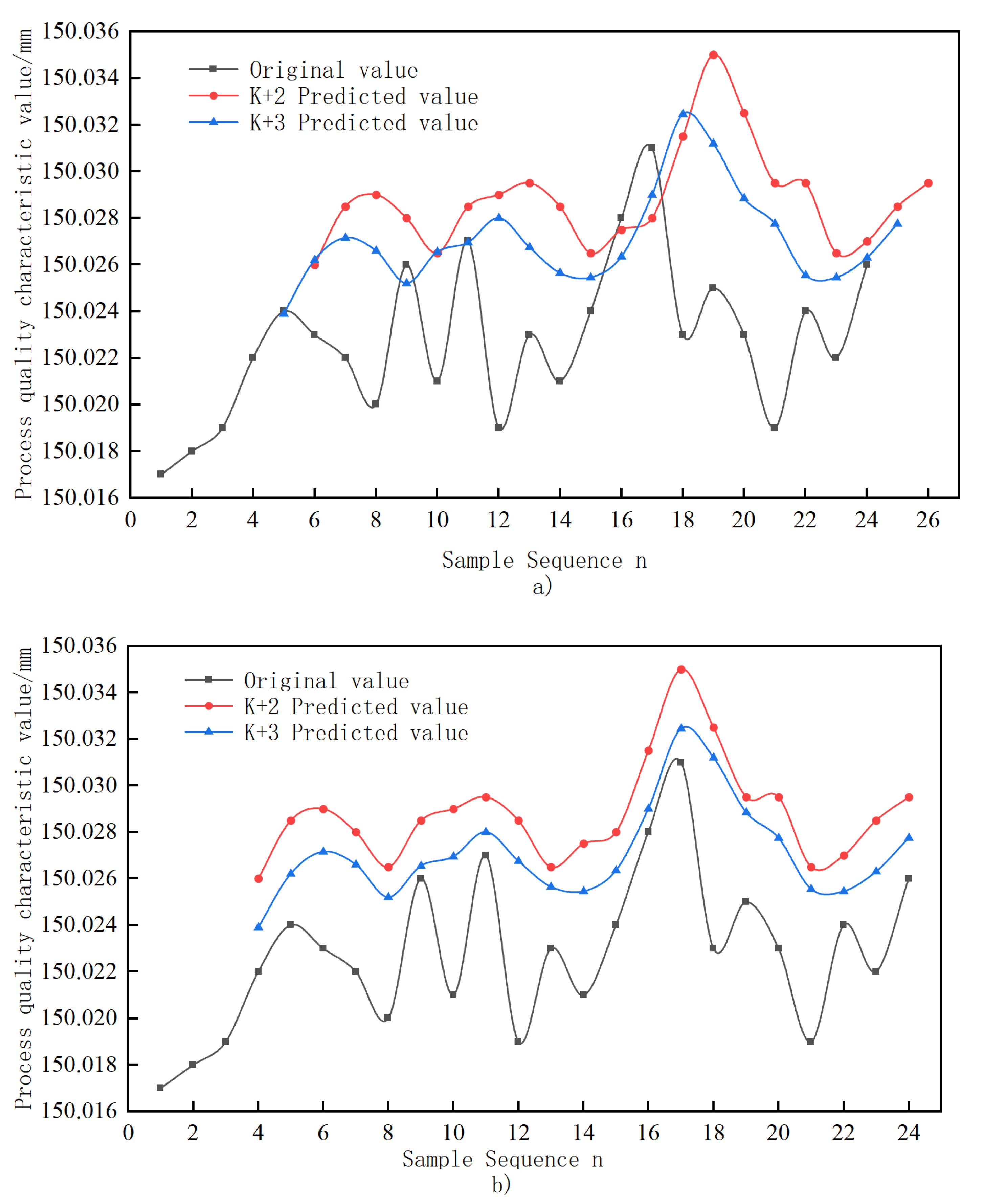
4.1.2. Verification of Dynamic Prediction of Work Process Quality Feature Values
4.2. Principle of Optimization of Neural Network Prediction Algorithm
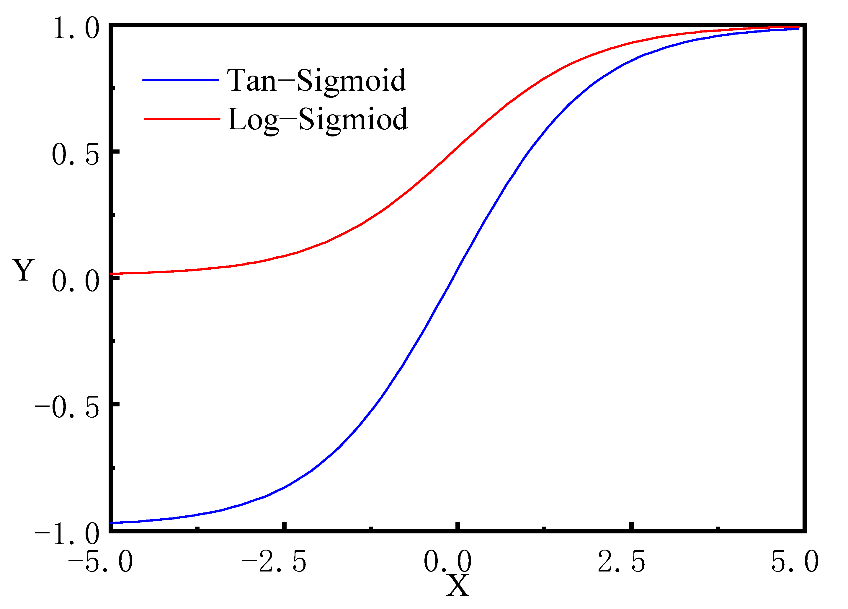
4.2.1. Selection of Transfer Functions
4.2.2. Pre-Feedback Propagation of the BP Neural Network
4.3. GM(1,1)-BP Combined Prediction Optimization
4.3.1. Residual Data Processing and Selection
4.3.2. Selection of Residual Values to Predict Model Parameters
- (1)
- Network initial parameters and the expected error value
- (2)
- Transfer function and training algorithm
- (3)
- Learning rate and determination of hidden layer nodes
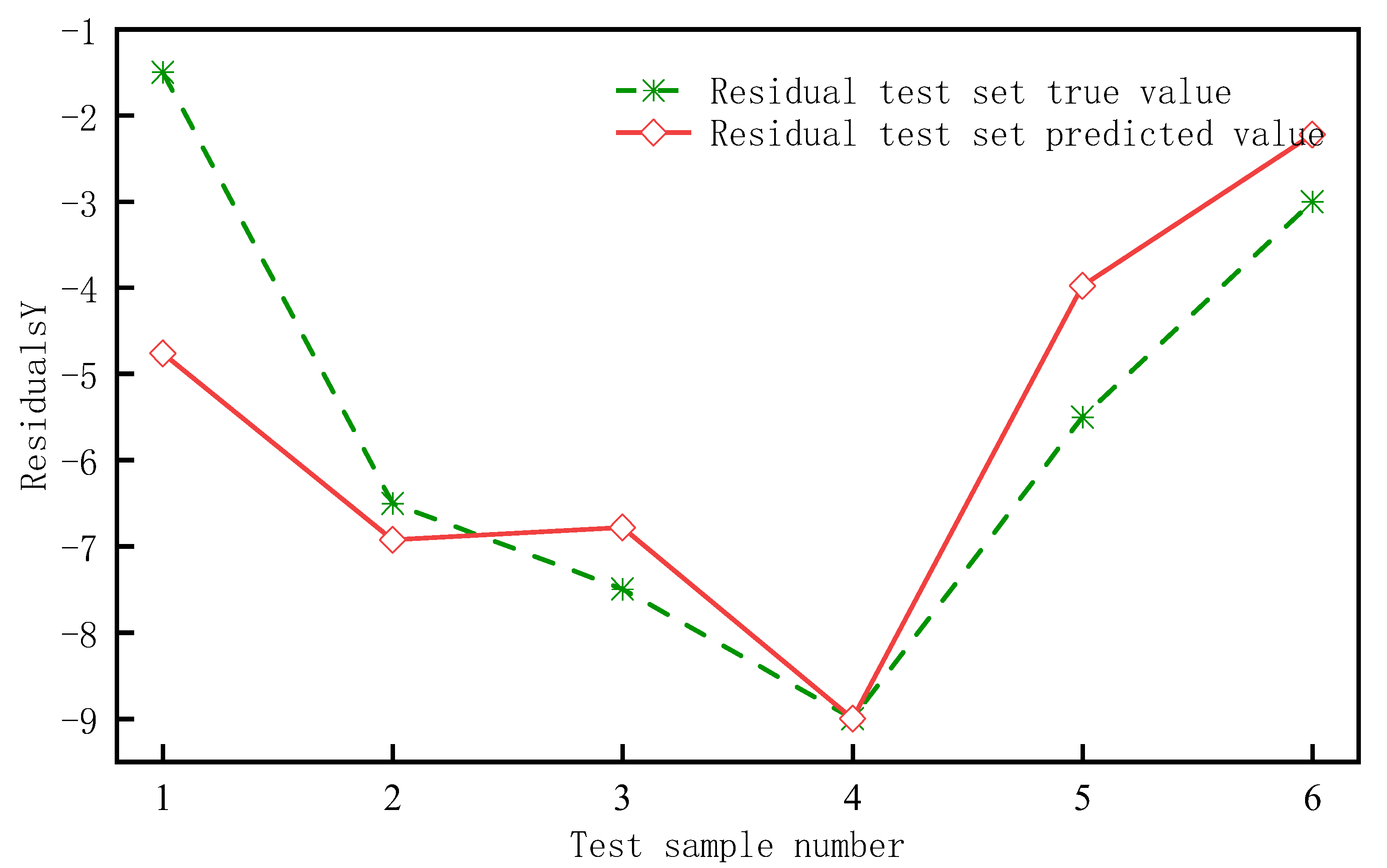
4.4. Example Illustration of Residual Value Prediction
- (1)
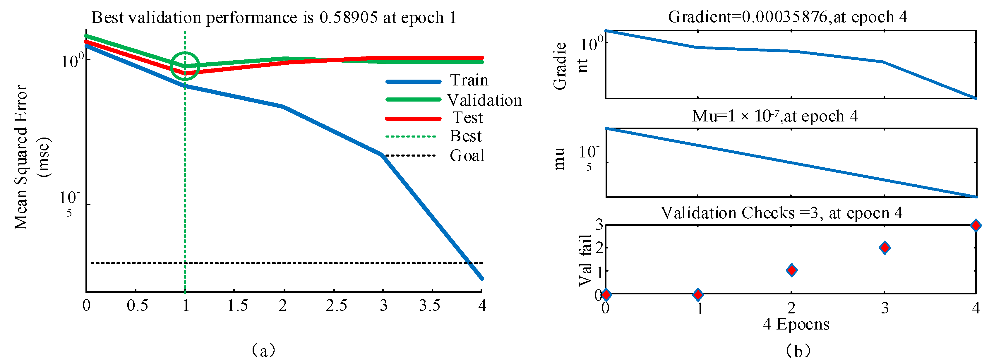
- Training and capability verification of the BP neural network model
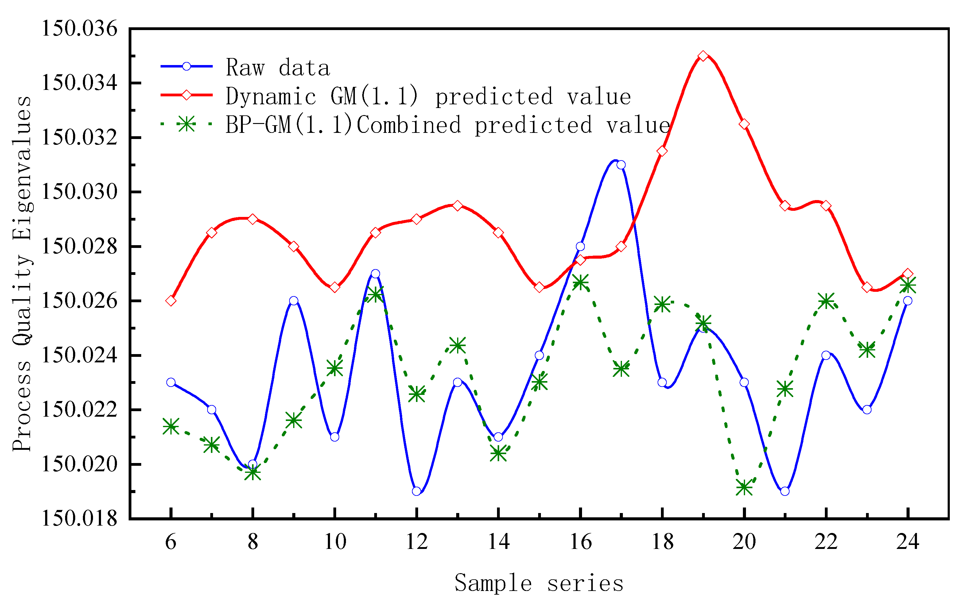
4.5. Combined Prediction Validation of BP-GM(1,1)
5. Process Quality Monitoring and Evaluation of Flexible Production Line for Spindle Housing
5.1. Joint Control Based on EWMA
5.2. Spindle Box Process Quality Case Analysis and Verification
6. Conclusions
- (1)
- A decision analysis model of process quality influencing factors of a spindle box flexible production line is established, and process quality control decisions are formulated. Through a comprehensive analysis of the process quality influencing factors, a hierarchical model of the spindle box process quality influencing factors is established, combined with the “5M1E” analysis method and fuzzy hierarchical analysis method, to analyze and make decisions on the influence of multiple factors. The fuzzy weight ranking value of each influencing factor is used to improve the process quality control decision of the spindle box flexible production line.
- (2)
- A combined prediction model of process quality characteristic values is established. The dynamic GM(1,1) predicts the fundamental process quality characteristic values and obtains the potential change trend of process quality. In order to avoid prediction failure due to large residual values, a BP neural network is used to correct the residuals of the predicted values. A model is obtained with predicted data close to the actual data variation. The average relative error is improved by 61% compared with dynamic GM(1,1), effectively reflecting the trend change of process quality characteristic values.
- (3)
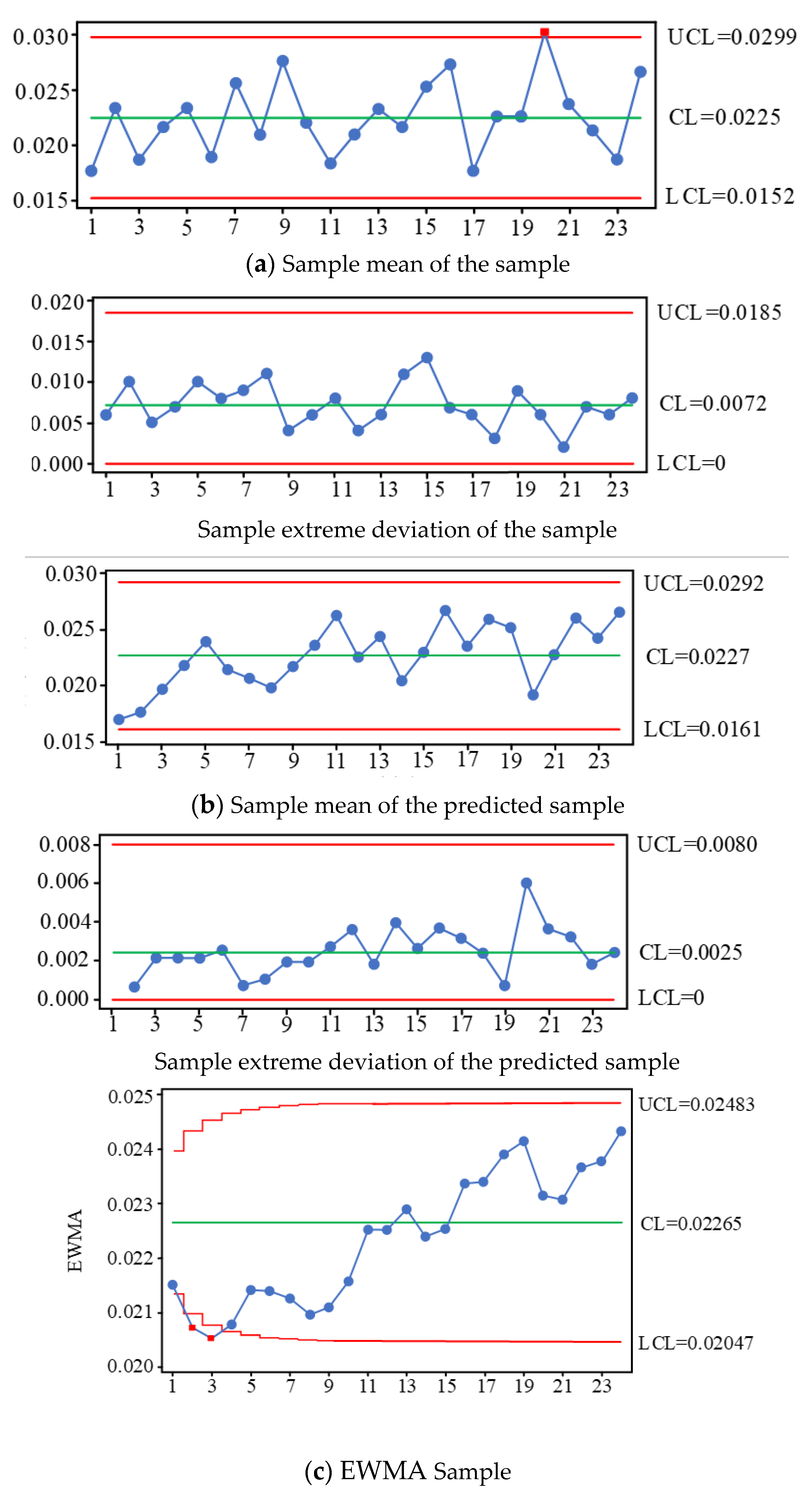
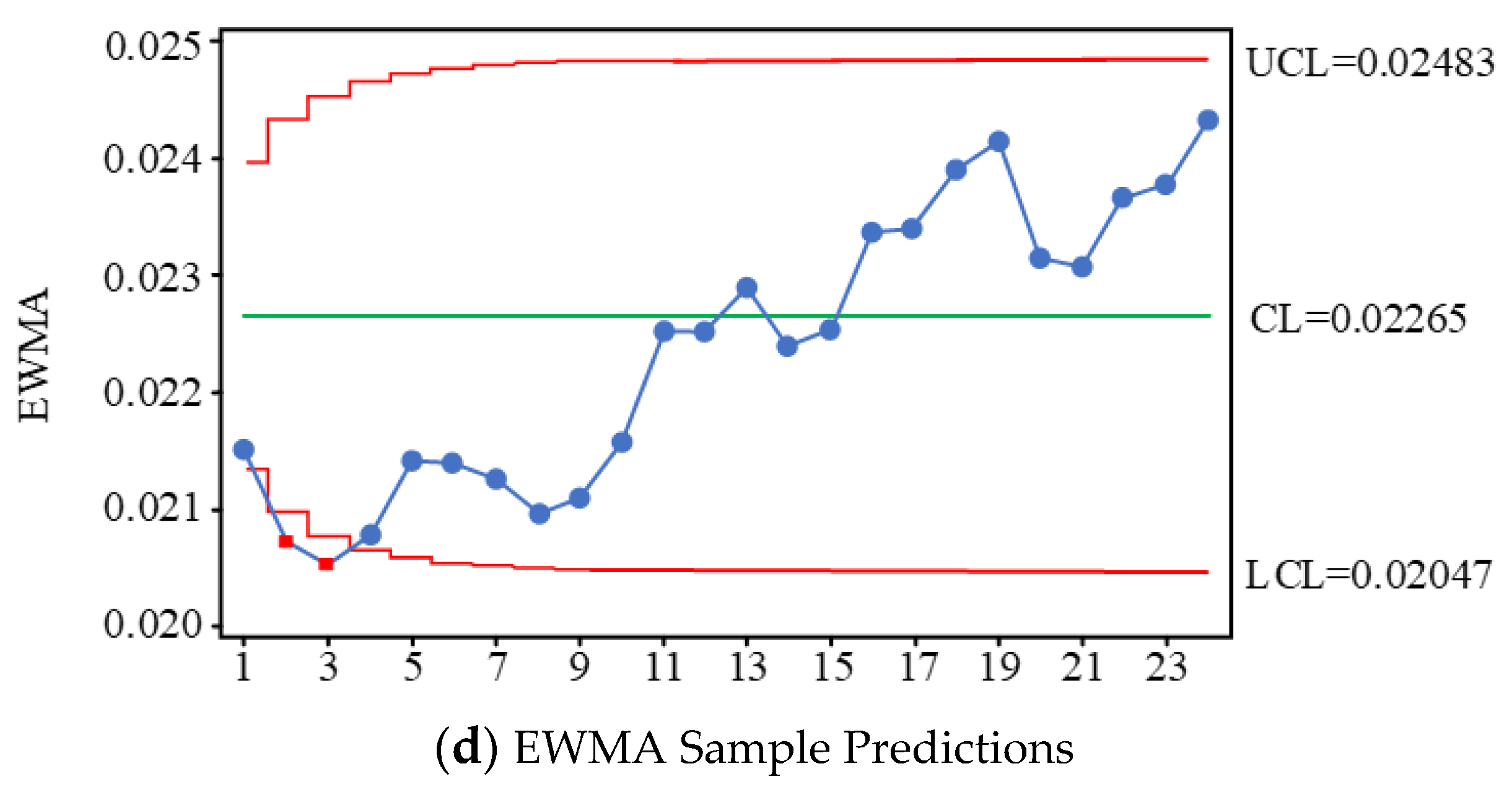
- A process quality monitoring and process capability assessment model is established for a spindle box flexible production line of spindle cases. Using the principle of statistical process control (SPC), the process quality control process of a spindle box flexible production line is developed, and multiple control charts are used to jointly determine whether there is an uncontrolled state or trend in process quality. The actual and predicted values of the process quality characteristics are analyzed by combining multiple control charts. Based on the actual data and predicted changes in quality characteristics, we use time weighted EWAM control charts in conjunction with average and extreme difference control charts to determine the production line’s current process quality status and to analyze the production line’s quality problems. The process quality is again monitored for potential out-of-control trends based on predicted data using multiple control charts jointly.
Author Contributions
Funding
Institutional Review Board Statement
Informed Consent Statement
Data Availability Statement
Conflicts of Interest
References
- Zhao, J.; Wei, T.; Song, L. ANSYS-based optimization of machine tool spindle box structure design. Mechatron. Prod. Dev. Innov. 2010, 23, 140–142. [Google Scholar] [CrossRef]
- Chen, A.; Wang, S.; Li, X. Mechanical Manufacturing Technology; Beijing Polytechnic University Press: Beijing, China, 2010. [Google Scholar]
- Zhu, Y.; Hu, K.; Song, X. Development and application of an online quality control system for precision copper tube production lines. Mech. Eng. Autom. 2016, 5, 150–151+155. [Google Scholar] [CrossRef]
- Guo, W.; Banerjee, A.G. Identification of key features using topological data analysis for accurate prediction of manufacturing system outputs. J. Manuf. Syst. 2017, 43, 225–234. [Google Scholar] [CrossRef]
- Li, A.D.; He, Z. Multiobjective feature selection for key quality characteristic identification in production processes using a nondominated-sorting-based whale optimization algorithm. Comput. Ind. Eng. 2020, 149, 106852. [Google Scholar] [CrossRef]
- Song, W.; Cao, W.; Hu, W.; Wu, M. Identification of multiple operating modes based on fused features for continuous annealing processes. Inf. Sci. 2020, 534, 85–96. [Google Scholar] [CrossRef]
- Liu, T.; Liu, R.; Duan, G. A principle-empirical model based on Bayesian network for quality improvement in mechanical products development. Comput. Ind. Eng. 2020, 149, 106807. [Google Scholar] [CrossRef]
- Xu, W.; Guo, C.; Guo, S.; Wang, L.; Li, X. A novel quality comprehensive evaluation method based on product gene for solving the manufacturing quality tracking problem of large equipment. Comput. Ind. Eng. 2021, 152, 107032. [Google Scholar] [CrossRef]
- Colledani, M.; Tolio, T.; Fischer, A.; Lung, B.; Lanza, G.; Schmitt, R.; Váncza, J. Design and management of manufacturing systems for production quality. CIRP Ann. 2014, 63, 773–796. [Google Scholar] [CrossRef]
- Liu, J.; Cao, X.; Zhou, H.; Li, L.; Liu, X.; Zhao, P.; Dong, J. A digital twin-driven approach towards traceability and dynamic control for processing quality. Adv. Eng. Inform. 2021, 50, 101395. [Google Scholar] [CrossRef]
- Pang, J.; Zhang, N.; Xiao, Q.; Qi, F.; Xue, X. A new intelligent and data-driven product quality control system of industrial valve manufacturing process in CPS. Comput. Commun. 2021, 175, 25–34. [Google Scholar] [CrossRef]
- Sikder, S.; Mukherjee, I.; Panja, S.C. A synergistic Mahalanobis–Taguchi system and support vector regression based predictive multivariate manufacturing process quality control approach. J. Manuf. Syst. 2020, 57, 323–337. [Google Scholar] [CrossRef]
- Radcliffe, A.J.; Reklaitis, G.V. Bayesian hierarchical modeling for online process monitoring and quality control, with application to real time image data. Comput. Chem. Eng. 2021, 154, 107446. [Google Scholar] [CrossRef]
- Li, M.; Huang, G.Q. Production-intralogistics synchronization of industry 4.0 flexible assembly lines under graduation intelligent manufacturing system. Int. J. Prod. Econ. 2021, 241, 108272. [Google Scholar] [CrossRef]
- Frye, M.; Gyulai, D.; Bergmann, J.; Schmitt, R.H. Production rescheduling through product quality prediction. Procedia Manuf. 2021, 54, 142–147. [Google Scholar] [CrossRef]
- Xu, H.; Lan, K.; Ma, Y. Accuracy-oriented identification method and application of key processes in segmented workshops. Mar. Eng. 2020, 42, 141–146. [Google Scholar] [CrossRef]
- Wei, Y.; Chen, Y.; Suo, S. A method for evaluating complex product architectures based on modularity and equilibrium. J. Eng. Des. 2021, 28, 527–538. [Google Scholar] [CrossRef]
- Zhang, F.; He, J.; Su, J. Modeling and analysis of part machining feature evolution ab initio networks based on multi-process manufacturing processes. J. Beijing Univ. Technol. 2017, 43, 833–839. [Google Scholar] [CrossRef]
- Yang, W.; Xie, Y.; Kun, Y. Prediction of hydrate generation in compressed cooling storage systems based on grey correlation BP neural networks. Chem. Prog. 2021, 40, 664–670. [Google Scholar]
- Ying, G. Research on Quality Control and Prediction Technology for Flexible Production Line Processes. Master’s Thesis, Chongqing University, Chongqing, China, 2018. [Google Scholar] [CrossRef]
- Yang, X.; Xiao, F. An improved gravity model to identify influential nodes in complex networks based on k-shell method. Knowl.-Based Syst. 2021, 227, 107198. [Google Scholar] [CrossRef]
- Ma, Y.; Li, L.; Yin, Z.; Chai, A.; Li, M.; Bi, Z. Research and application of network status prediction based on BP neural network for intelligent production line. Procedia Comput. Sci. 2021, 183, 189–196. [Google Scholar] [CrossRef]


| Feature Code | Code Meaning | Number of Features |
|---|---|---|
| XCMZ | The left side of the box | 1 |
| XCMY | The right side of the box | 1 |
| DWCMZ | The left side of the left rail | 1 |
| DWCMY | Right rail outer side | 1 |
| DWCMY_Q | The Notch on the outside of the right rail | 3 |
| XCMZ_K | Bottom hole on the left side of the box | 8 |
| XCMY_K | Bottom hole of the right side of the box | 10 |
| DWCMZ_K | Bottom hole of the outer side of the left rail | 4 |
| DWCMY_K | Bottom hole of the outer side of the right rail | 4 |
| DWCMY_QK | Bottom hole of the outer rail outer side notch | 6 |
| XCMY_GK | The right side of the box processes positioning holes | 2 |
| XCMZ_GK | Process positioning holes on the left side of the box | 3 |
| DM | Box top surface | 1 |
| ZZM | Spindle mounting surface | 1 |
| DGM | Guide rail mounting end face | 2 |
| DGM_L | Guide rail mounting elevation | 4 |
| DJDM | Motor base bottom surface | 1 |
| PHM | Balancing cylinder mounting end face | 1 |
| PHM_K | Balancing cylinder mounting end face bottom hole | 6 |
| DJM | The motor mount end face | 1 |
| DM_K | Bottom hole of the top surface of the box | 28 |
| ZZM_K | Bottom hole of the spindle mounting end | 8 |
| DGM_K | Bottom hole of mounting end of the guide rail | 7 |
| PHM_K | Bottom hole of the balancing cylinder mounting end | 6 |
| DJM_K | Bottom hole of the motor mounting end | 5 |
| ZZK | Spindle hole | 1 |
| LMZK | Motor mount hole | 24 |
| Serial Number | Feature ID | Nodality | Number of Nodes | Centrality Mean | The Average Value of Each Index |
|---|---|---|---|---|---|
| 1 | DGM | 12.62 | 15.03 | 32.05 | 20.15 |
| 2 | ZZK | 15.23 | 14.38 | 24.36 | 18.32 |
| 3 | DGM_L | 12.65 | 17.12 | 16.32 | 15.26 |
| 4 | DJM | 12.64 | 9.88 | 8.32 | 10.12 |
| 5 | ZZM | 7.36 | 7.65 | 10.32 | 8.63 |
| 6 | DM | 2.21 | 2.26 | 2.86 | 2.52 |
| 7 | XCMY | 2.21 | 1.18 | 2.07 | 1.66 |
| 8 | XCMZ | 1.82 | 0.98 | 1.16 | 1.28 |
| 9 | HKM | 0.56 | 0.92 | 0.96 | 0.88 |
| 10 | LMDM | 0.56 | 0.92 | 0.96 | 0.88 |
| 11 | PHM | 0.46 | 0.88 | 0.81 | 0.78 |
| 12 | LMM | 0.46 | 0.88 | 0.81 | 0.78 |
| 13 | LMZK | 0.46 | 0.88 | 0.81 | 0.78 |
| 14 | DWCMY_K | 0.21 | 0.31 | 0.22 | 0.26 |
| 15 | DWCMY_QK | 0.18 | 0.24 | 0.30 | 0.24 |
| 16 | XCMY_GK | 0.18 | 0.24 | 0.30 | 0.24 |
| 17 | LMZK | 0.12 | 0.22 | 0.26 | 0.20 |
| 18 | DM_K | 0.16 | 0.16 | 0.16 | 0.16 |
| 19 | ZZM_K | 0.12 | 0.12 | 0.12 | 0.12 |
| 20 | HKM_K | 0.09 | 0.09 | 0.09 | 0.09 |
| 21 | PHM_K | 0.09 | 0.09 | 0.09 | 0.09 |
| 22 | LMM_K | 0.07 | 0.07 | 0.07 | 0.07 |
| 23 | ZZK | 0.04 | 0.04 | 0.04 | 0.04 |
| 24 | LMZK | 0.04 | 0.04 | 0.04 | 0.04 |
| U | A1 | A2 | … | An |
|---|---|---|---|---|
| A1 | a11 | a12 | … | a1n |
| A2 | a21 | a22 | … | a2n |
| ⋮ | ⋮ | ⋮ | ⋮ | ⋮ |
| An | an1 | an2 | … | ann |
| Scale | Definition | Meaning |
|---|---|---|
| 0.1 | Indicator i compared to indicator j | j is more important than i in the extreme |
| 0.2 | Indicator i compared to indicator j | j is more strongly important than i |
| 0.3 | Indicator i compared to indicator j | j is significantly more important than i |
| 0.4 | Indicator i compared to indicator j | j is slightly more important than i |
| 0.5 | Indicator i compared to indicator j | j is as important as i |
| 0.6 | Indicator i compared to indicator j | j is slightly more important than i |
| 0.7 | Indicator i compared to indicator j | j is significantly more important than i |
| 0.8 | Indicator i compared to indicator j | j is more strongly important than i |
| 0.9 | Indicator i compared to indicator j | j is more extremely important than i |
| U | A1 | A2 | A3 | A4 | A5 |
|---|---|---|---|---|---|
| A1 | 0.5 | 0.7 | 0.7 | 0.6 | 0.8 |
| A2 | 0.3 | 0.5 | 0.4 | 0.3 | 0.4 |
| A3 | 0.3 | 0.6 | 0.5 | 0.6 | 0.6 |
| A4 | 0.4 | 0.7 | 0.4 | 0.5 | 0.6 |
| A5 | 0.2 | 0.6 | 0.4 | 0.4 | 0.5 |
| A1 | B1 | B2 | B3 | |
|---|---|---|---|---|
| B1 | 0.5 | 0.6 | 0.4 | |
| B2 | 0.4 | 0.5 | 0.3 | |
| B3 | 0.6 | 0.7 | 0.5 | |
| A2 | B4 | B5 | B6 | |
| B4 | 0.5 | 0.6 | 0.7 | |
| B5 | 0.4 | 0.5 | 0.6 | |
| B6 | 0.3 | 0.4 | 0.5 | |
| A3 | B7 | B8 | ||
| B7 | 0.5 | 0.4 | ||
| B8 | 0.6 | 0.5 | ||
| A4 | B9 | B10 | B11 | |
| B9 | 0.5 | 0.4 | 0.3 | |
| B10 | 0.6 | 0.5 | 0.4 | |
| B11 | 0.7 | 0.6 | 0.5 | |
| A5 | B12 | B13 | B14 | B15 |
| B12 | 0.5 | 0.4 | 0.6 | 0.7 |
| B13 | 0.6 | 0.5 | 0.6 | 0.8 |
| B14 | 0.4 | 0.4 | 0.5 | 0.6 |
| B15 | 0.3 | 0.2 | 0.4 | 0.5 |
| Indicator Layer A | Indicator Weights | Sub-Indicator Layer B | Sub-Indicator Weights | Total Weights |
|---|---|---|---|---|
| Machinery and Equipment | 0.225 | Maintenance | 0.333 | 0.075 |
| Tool management | 0.296 | 0.067 | ||
| Operation calibration | 0.371 | 0.083 | ||
| Materials | 0.181 | Raw material quality | 0.371 | 0.067 |
| Process inspection | 0.333 | 0.060 | ||
| Material economy | 0.296 | 0.054 | ||
| Methods | 0.203 | Reasonable tooling solutions | 0.450 | 0.091 |
| Reasonable process planning | 0.550 | 0.112 | ||
| Measurement | 0.203 | Measurement accuracy requirements | 0.296 | 0.060 |
| Maintenance or replacement | 0.333 | 0.068 | ||
| Measurement process specification | 0.371 | 0.075 | ||
| Environment | 0.188 | Dust contamination | 0.261 | 0.049 |
| Safety | 0.278 | 0.053 | ||
| Recyclability | 0.244 | 0.046 | ||
| Vibration noise | 0.217 | 0.041 |
| No. | Main Influencing Factors | Control Methods and Measures |
|---|---|---|
| 1 | Reasonable Tooling Solutions | 1. Regularly check whether the horizontal machining center fixture is damaged 2. Check that the fixture is reasonable and correct before machining 3. Check that the jig adjustment top position is in place |
| 2 | Reasonable process planning | 1. Regularly analyze the quality data of the spindle box for process improvement 2. Stop production to repair abnormal process problems 3. Repeatedly determine the process for different specifications of customized spindle cases |
| 3 | Equipment operation verification | 1. Horizontal machining center repair and calibration 2. Calibration of fixed-point positioning of the AGV trolley operation 3. Robot gripping and placement position verification 4. Calibration of the collaboration between the three-dimensional exchange device and the transportation line |
| Serial Number | Raw Date/mm | Serial Number | Raw Date/mm | Serial Number | Raw Date/mm |
|---|---|---|---|---|---|
| 1 | 150.017 | 9 | 150.026 | 17 | 150.031 |
| 2 | 150.018 | 10 | 150.021 | 18 | 150.028 |
| 3 | 150.019 | 11 | 150.027 | 19 | 150.025 |
| 4 | 150.022 | 12 | 150.019 | 20 | 150.023 |
| 5 | 150.024 | 13 | 150.023 | 21 | 150.021 |
| 6 | 150.023 | 14 | 150.021 | 22 | 150.024 |
| 7 | 150.022 | 15 | 150.024 | 23 | 150.022 |
| 8 | 150.020 | 16 | 150.028 | 24 | 150.026 |
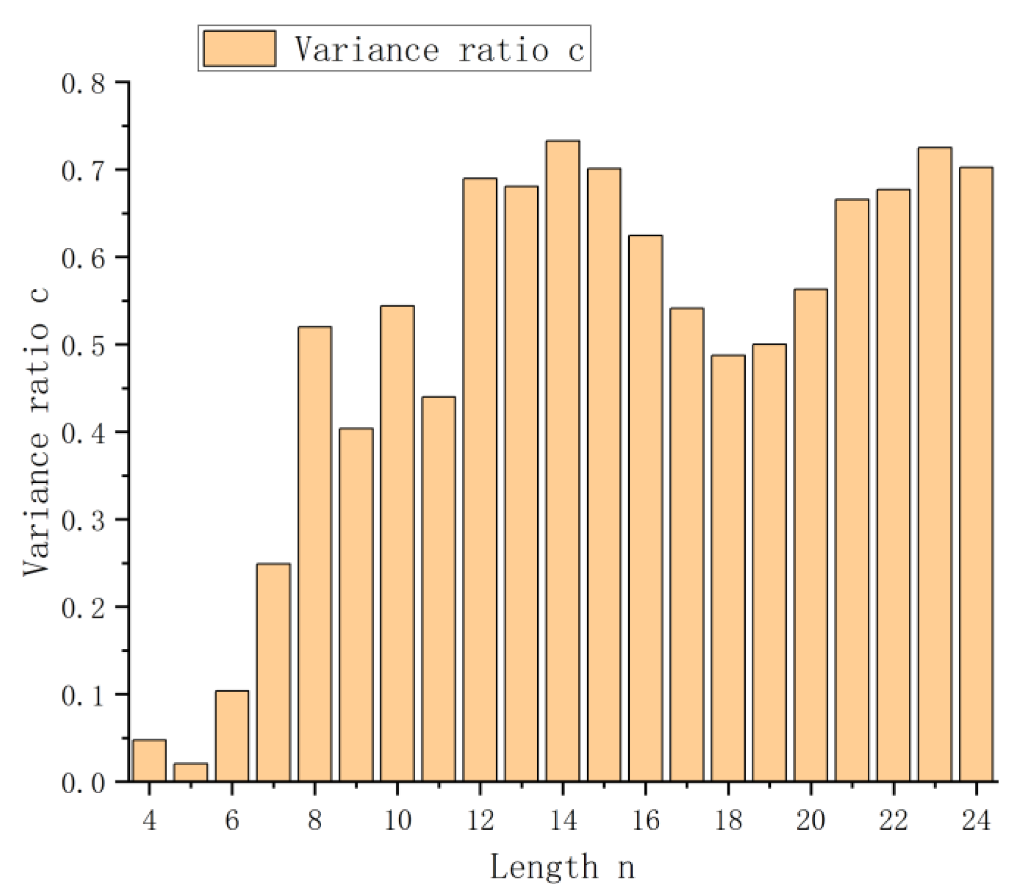
| n | C | n | C | n | C |
|---|---|---|---|---|---|
| 4 | 0.0476 | 11 | 0.4399 | 18 | 0.4874 |
| 5 | 0.0206 | 12 | 0.6895 | 19 | 0.5003 |
| 6 | 0.1036 | 13 | 0.6807 | 20 | 0.5631 |
| 7 | 0.2491 | 14 | 0.7328 | 21 | 0.6655 |
| 8 | 0.5201 | 15 | 0.7012 | 22 | 0.6771 |
| 9 | 0.4036 | 16 | 0.6247 | 23 | 0.7252 |
| 10 | 0.5438 | 17 | 0.5412 | 24 | 0.7022 |
| Group Number | Input Parameter Set | Output Parameter Set | ||||
|---|---|---|---|---|---|---|
| 1 | 0.0 | 0.4 | −0.7 | 0.2 | 0.1 | −3.0 |
| 2 | 0.4 | −0.7 | 0.2 | 0.1 | −3.0 | −6.5 |
| 3 | −0.7 | 0.2 | 0.1 | −3.0 | −6.5 | −9.0 |
| 4 | 0.2 | 0.1 | −3.0 | −6.5 | −9.0 | −2.0 |
| 5 | 0.1 | −3.0 | −6.5 | −9.0 | −2.0 | −5.5 |
| 6 | −3.0 | −6.5 | −9.0 | −2.0 | −5.5 | −1.5 |
| 7 | −6.5 | −9.0 | −2.0 | −5.5 | −1.5 | −10.0 |
| 8 | −9.0 | −2.0 | −5.5 | −1.5 | −10 | −6.5 |
| 9 | −2.0 | −5.5 | −1.5 | −10.0 | −6.5 | −7.5 |
| 10 | −5.5 | −1.5 | −10.0 | −6.5 | −7.5 | −2.5 |
| 11 | −1.5 | −10 | −6.5 | −7.5 | −2.5 | 0.5 |
| 12 | −10.0 | −6.5 | −7.5 | −2.5 | 0.5 | 3.0 |
| 13 | −6.5 | −7.5 | −2.5 | 0.5 | 3.0 | −8.5 |
| 14 | −7.5 | −2.5 | 0.5 | 3.0 | −8.5 | −10.0 |
| 15 | −2.5 | 0.5 | 3.0 | −8.5 | −10.0 | −9.5 |
| 16 | 0.5 | 3.0 | −8.5 | −10.0 | −9.5 | −10.5 |
| 17 | 3.0 | −8.5 | −10.0 | −9.5 | −10.5 | −5.5 |
| 18 | −8.5 | −10 | −9.5 | −10.5 | −5.5 | −4.5 |
| 19 | −10.0 | −9.5 | −10.5 | −5.5 | −4.5 | −1.0 |
| Learning Rate | Number of Implicit Layer Nodes | |||||||
|---|---|---|---|---|---|---|---|---|
| 5 | 6 | 7 | 8 | 9 | 10 | 11 | 12 | |
| 0.001 | 3.609 | 2.686 | 2.689 | 4.391 | 1.872 | 3.390 | 1.020 | 1.970 |
| 0.01 | 5.599 | 1.770 | 6.091 | 3.886 | 2.993 | 3.714 | 2.433 | 3.274 |
| 0.1 | 6.183 | 1.585 | 2.846 | 3.430 | 2.339 | 3.189 | 5.540 | 3.626 |
| 0.2 | 3.563 | 2.079 | 2.551 | 2.381 | 2.459 | 9.471 | 3.7587 | 3.139 |
| 0.5 | 5.054 | 6.004 | 3.377 | 3.120 | 1.477 | 5.903 | 1.714 | 4.540 |
| Number of Groups | Test Set Input Vector | Test Set Output Vector | |||||
|---|---|---|---|---|---|---|---|
| 1 | −3.0 | −6.5 | −9.0 | −2.0 | −5.5 | −3.0 | −1.5 |
| 2 | −9.0 | −2.0 | −5.5 | −1.5 | −10.0 | −9.0 | −6.5 |
| 3 | −2.0 | −5.5 | −1.5 | −10.0 | −6.5 | −2.0 | −7.5 |
| 4 | −0.7 | 0.2 | 0.1 | −3.0 | −6.5 | −0.7 | −9.0 |
| 5 | 3.0 | −8.5 | −10.0 | −9.5 | −10.5 | 3.0 | −5.5 |
| 6 | 0.0 | 0.4 | −0.7 | 0.2 | 0.1 | 0.0 | −3.0 |
| Sample Number | Original Value/mm | Dynamic GM(1,1) Predicted Value/mm | Dynamic GM(1,1) Δ | Combined Predicted Value/mm | Combined Forecast Δ |
|---|---|---|---|---|---|
| 6 | 150.023 | 150.0260 | 0.00200% | 150.0214 | 0.00107% |
| 7 | 150.022 | 150.0285 | 0.00433% | 150.0207 | 0.00086% |
| 8 | 150.020 | 150.0290 | 0.00600% | 150.0197 | 0.00019% |
| 9 | 150.026 | 150.0280 | 0.00133% | 150.0216 | 0.00291% |
| 10 | 150.021 | 150.0265 | 0.00367% | 150.0235 | 0.00169% |
| 11 | 150.027 | 150.0285 | 0.00100% | 150.0262 | 0.00051% |
| 12 | 150.019 | 150.0290 | 0.00667% | 150.0226 | 0.00239% |
| 13 | 150.023 | 150.0295 | 0.00433% | 150.0244 | 0.00091% |
| 14 | 150.021 | 150.0285 | 0.00500% | 150.0204 | 0.00040% |
| 15 | 150.024 | 150.0265 | 0.00167% | 150.0230 | 0.00065% |
| 16 | 150.028 | 150.0275 | 0.00033% | 150.0267 | 0.00088% |
| 17 | 150.031 | 150.0280 | 0.00200% | 150.0235 | 0.00499% |
| 18 | 150.023 | 150.0315 | 0.00567% | 150.0259 | 0.00192% |
| 19 | 150.025 | 150.0350 | 0.00667% | 150.0252 | 0.00012% |
| 20 | 150.023 | 150.0325 | 0.00633% | 150.0190 | 0.00256% |
| 21 | 150.019 | 150.0295 | 0.00700% | 150.0230 | 0.00252% |
| 22 | 150.024 | 150.0295 | 0.00367% | 150.0260 | 0.00133% |
| 23 | 150.022 | 150.0265 | 0.00300% | 150.0240 | 0.00147% |
| 24 | 150.026 | 150.0270 | 0.00067% | 150.0266 | 0.00039% |
| = 0.00396% | = 0.00154% |
| Serial Number | Measured Value/mm | Deviation Conversion Value/mm | Serial Number | Measured Value/mm | Deviation Conversion Value/mm |
|---|---|---|---|---|---|
| 1 | 150.017 150.015 150.021 | 0.017 0.020 0.021 | 13 | 150.021 150.022 150.027 | 0.021 0.022 0.027 |
| 2 | 150.018 150.024 150.028 | 0.018 0.024 0.021 | 14 | 150.027 150.016 150.022 | 0.027 0.016 0.022 |
| 3 | 150.019 150.016 150.021 | 0.019 0.016 0.021 | 15 | 150.019 150.025 150.032 | 0.019 0.025 0.032 |
| 4 | 150.022 150.018 150.025 | 0.022 0.018 0.025 | 16 | 150.023 150.029 150.030 | 0.023 0.029 0.030 |
| 5 | 150.024 150.028 150.018 | 0.024 0.028 0.018 | 17 | 150.021 150.015 150.017 | 0.021 0.015 0.017 |
| 6 | 150.023 150.015 150.019 | 0.023 0.015 0.019 | 18 | 150.024 150.021 150.023 | 0.024 0.021 0.023 |
| 7 | 150.022 150.024 150.031 | 0.022 0.024 0.021 | 19 | 150.028 150.019 150.021 | 0.028 0.019 0.021 |
| 8 | 150.020 150.027 150.016 | 0.020 0.027 0.016 | 20 | 150.031 150.033 150.027 | 0.031 0.033 0.027 |
| 9 | 150.026 150.027 150.030 | 0.026 0.027 0.030 | 21 | 150.023 150.023 150.025 | 0.023 0.023 0.025 |
| 10 | 150.025 150.019 150.022 | 0.025 0.019 0.022 | 22 | 150.024 150.023 150.017 | 0.024 0.023 0.017 |
| 11 | 150.023 150.015 150.017 | 0.023 0.015 0.017 | 23 | 150.022 150.016 150.018 | 0.022 0.016 0.018 |
| 12 | 150.019 150.021 150.023 | 0.019 0.021 0.023 | 24 | 150.026 150.023 150.031 | 0.026 0.023 0.031 |
Disclaimer/Publisher’s Note: The statements, opinions and data contained in all publications are solely those of the individual author(s) and contributor(s) and not of MDPI and/or the editor(s). MDPI and/or the editor(s) disclaim responsibility for any injury to people or property resulting from any ideas, methods, instructions or products referred to in the content. |
© 2023 by the authors. Licensee MDPI, Basel, Switzerland. This article is an open access article distributed under the terms and conditions of the Creative Commons Attribution (CC BY) license (https://creativecommons.org/licenses/by/4.0/).
Share and Cite
Huang, B.; Yan, J.; Liu, X.; Xie, J.; Wang, J.; Liu, K.; Xu, Y.; Peng, G. Research on Process Quality Prediction and Control of Spindle Housings in Flexible Production Lines. Appl. Sci. 2023, 13, 8371. https://doi.org/10.3390/app13148371
Huang B, Yan J, Liu X, Xie J, Wang J, Liu K, Xu Y, Peng G. Research on Process Quality Prediction and Control of Spindle Housings in Flexible Production Lines. Applied Sciences. 2023; 13(14):8371. https://doi.org/10.3390/app13148371
Chicago/Turabian StyleHuang, Bo, Jiawei Yan, Xiang Liu, Jiacheng Xie, Jian Wang, Kang Liu, Yun Xu, and Gongli Peng. 2023. "Research on Process Quality Prediction and Control of Spindle Housings in Flexible Production Lines" Applied Sciences 13, no. 14: 8371. https://doi.org/10.3390/app13148371
APA StyleHuang, B., Yan, J., Liu, X., Xie, J., Wang, J., Liu, K., Xu, Y., & Peng, G. (2023). Research on Process Quality Prediction and Control of Spindle Housings in Flexible Production Lines. Applied Sciences, 13(14), 8371. https://doi.org/10.3390/app13148371