1. Research Background
A large concrete aqueduct with a total length of 1083.6 m is a key structure of a water supply project in eastern China. It has 21 spans with a 51.6 m equal span length. The structural feature of the aqueduct is shown in
Figure 1, and its main load-bearing components are comprised of arch trusses (concrete design strength C50), bent frames (C40) and moment frame supports (C40). The aqueduct was built in 2006, and after 17 years of operation without any safety monitoring measures, the management now plans to install an SHM on it.
The dynamic elastic modulus (
Ed) of concrete is of great interest in hydraulic structures. In the Chinese hydraulic concrete design code, the durability of concrete is evaluated by the reduction of
Ed, which can also provide appropriate dynamic parameters for the seismic analysis [
1,
2]. For high-, normal- and low-strength concrete, the ratios of the dynamic-to-static elastic modulus (
Ed/
Ec) are around 1.2, 1.3 and 1.4, respectively [
1]. According to the dynamic equilibrium equation, the natural vibration frequencies of a concrete structure are directly related to its concrete
Ed, which can be obtained from examining the dynamic responses of the structure on site.
Aqueducts are structurally similar, with bridges. Vibration-based (dynamic) tests have been considered as an effective approach to evaluate the structural health of bridges [
3]. Many previous studies focused on analyzing modal parameters (frequencies and shapes) through numerical models combined with field test results to identify and locate structural damages in bridges [
4,
5,
6,
7,
8]. Analyses of modal parameters were performed to assess significant negative effects on bridges due to structural rehabilitation [
9,
10], and some researchers conducted ambient and vehicle-induced vibration tests for a real bridge subject to various deliberately designed damage conditions [
11]. Besides full-scale applications, vibration tests were also used to evaluate local damages in decks and slab–girder connectors of bridges [
12,
13,
14] and assist in optimizing the boundary constraints of the structural FE models [
15]. In recent years, more researchers have employed machine learning, especially artificial neural networks, in the damage detection of bridges by exploiting in situ experimental and numerical analytical data [
16,
17,
18,
19], and particularly due to its maturity in both theory and performance as well as flexibility in network architecture, BP (back-propagation) neural network has been widely used [
20,
21,
22,
23]. Efforts have also been made in applying convolutional neural networks (CNNs) to visually reveal structural defects in bridge girders [
24,
25].
The purpose of this study was to determine the general concrete
Ed status for the main load-bearing components (arch trusses, bent frames and moment frame supports) of the aqueduct, thus to set an evaluation baseline before the SHM implementation. So with the long-term concrete
Ed data accumulated from the subsequent monitoring, it is possible to track the development of the health status of this old aqueduct. This task is completed by the application of in situ dynamic tests and the BP neural network trained with analytical data from a full-scale numerical model (see
Figure 2), as discussed below.
2. Dynamic Tests of the Real Structure
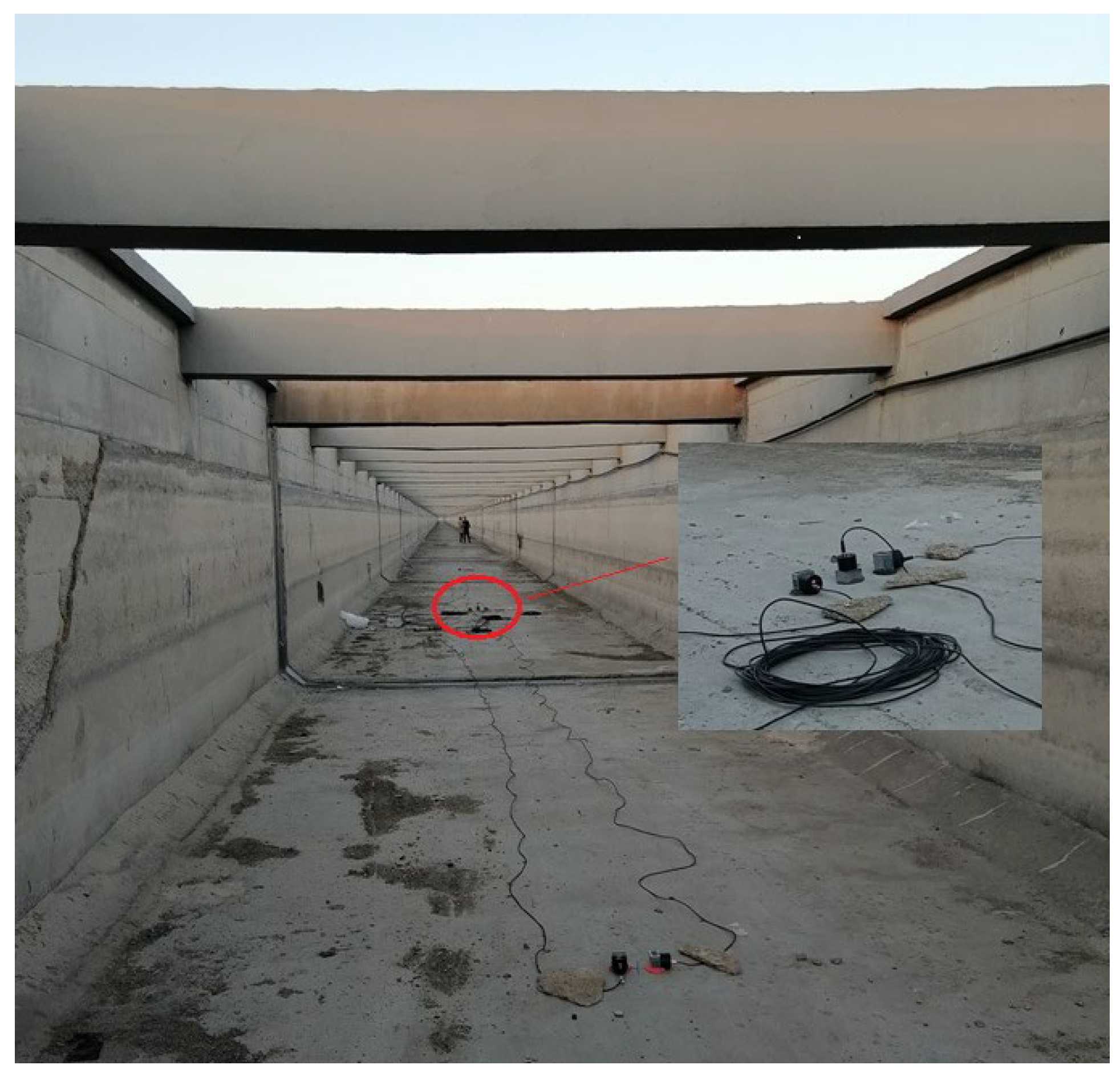
In situ dynamic tests were performed to investigate the structural vibration characteristics of the aqueduct under the natural wind excitation. Velocity transducers were installed on the top surface of the bottom slabs of the U-shaped flumes at locations of 1/4, 1/2 and 3/4 spans for span 6, 8, 10 and 14 (see
Figure 2). A three-directional transducer layout, as shown in
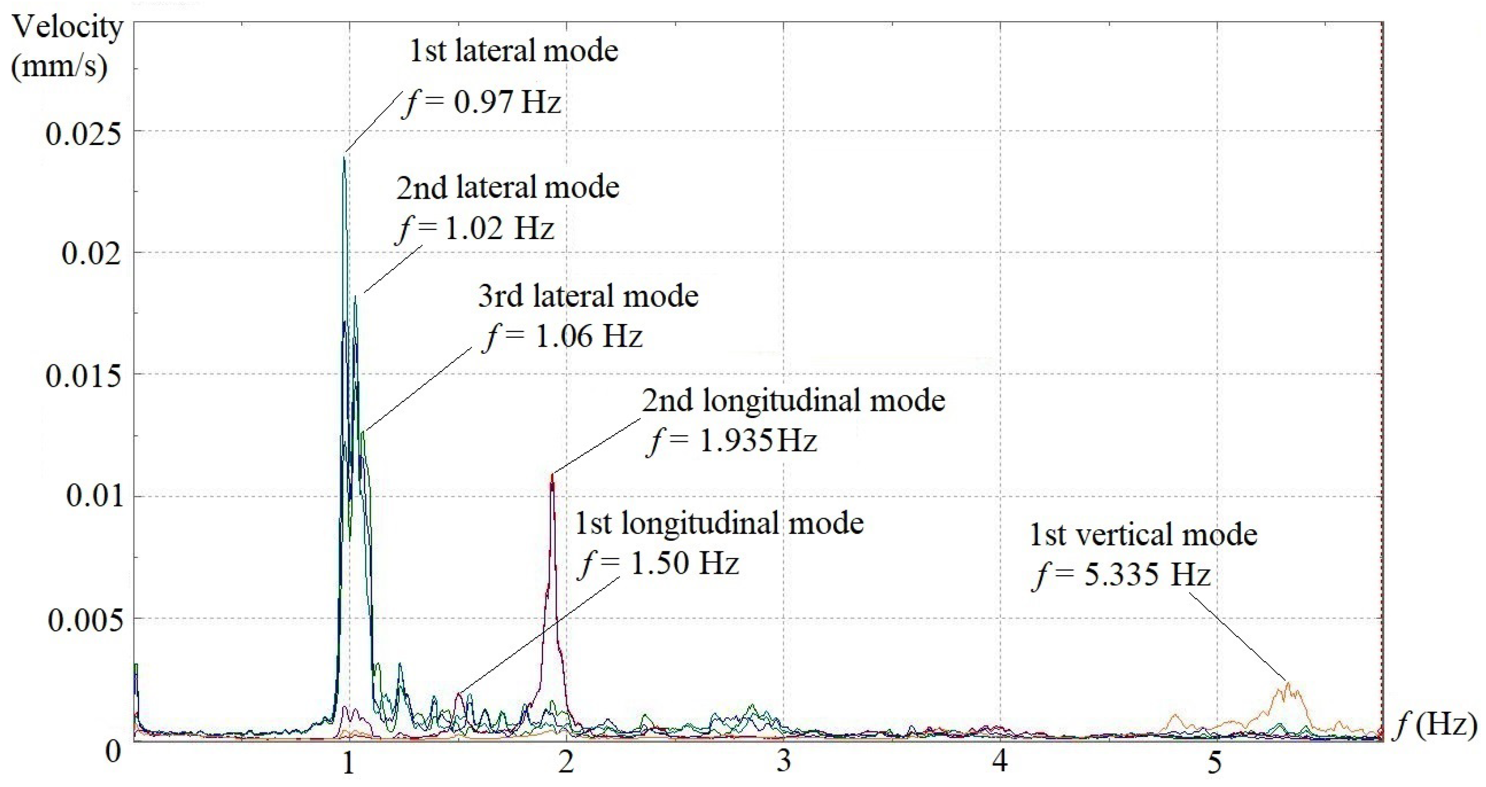
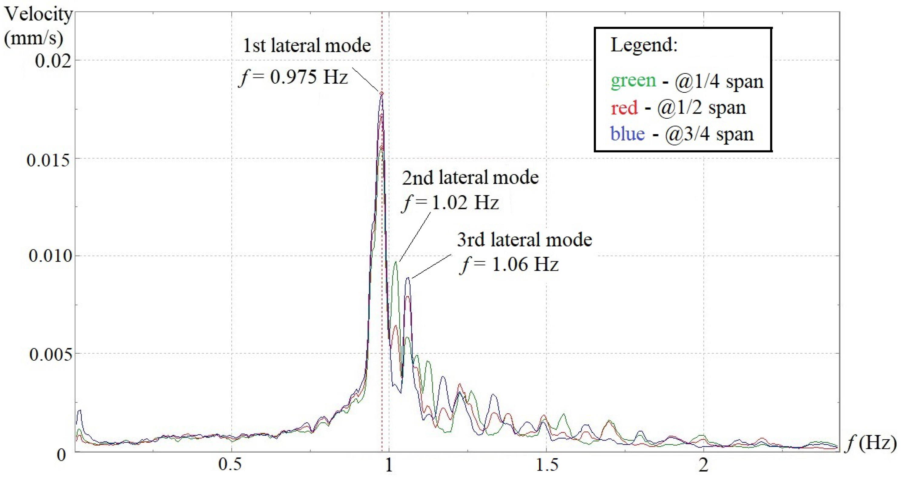
Figure 3, was adopted at the 1/2 span along the lateral, longitudinal and vertical directions, whereas only lateral and longitudinal transducers were placed at 1/4 and 3/4 spans. The 4 spans were tested individually. A sampling frequency of 20 Hz, which corresponds to a sampling interval of 50 ms, was set, and the total sampling time was fixed as 10 min. In the final data processing, an FFT point of 4096, Hanning window and 1/2 data-segment overlap were chosen, which gave rise to a 0.005 Hz resolution in the frequency domain spectra. Under the aforementioned testing setups and analysis parameters, the velocity spectra in the frequency domain for all transducers in three directions of the 4 spans are shown in
Figure 4,
Figure 5,
Figure 6 and
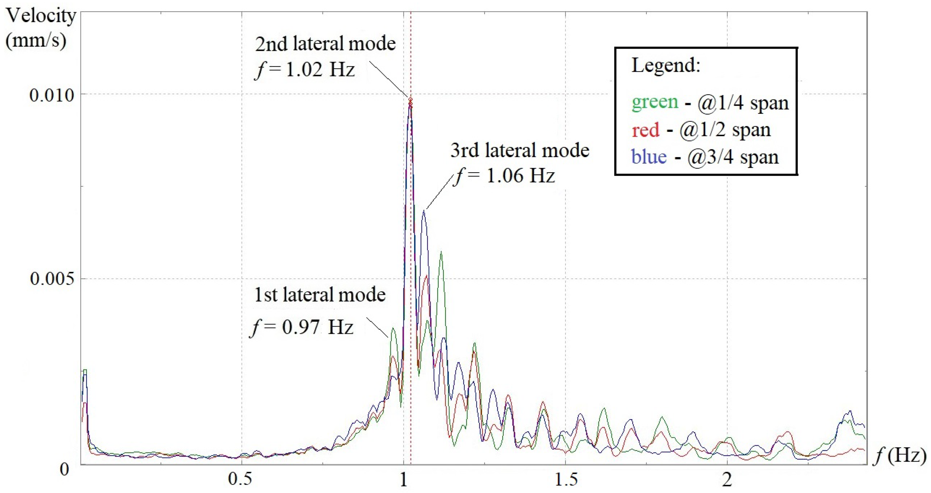
Figure 7. To better show the consistency of test results, two typical spectra obtained from 3 lateral sensors (@ 1/4, 1/2 and 3/4 span) on span #8 and #10 are also provided (see
Figure 8 and
Figure 9). On the velocity spectrum of each span, the peak amplitude frequencies obtained from the data collected by more than 2 transducers in the same direction (lateral or longitudinal) but at different locations well coincide with one another.
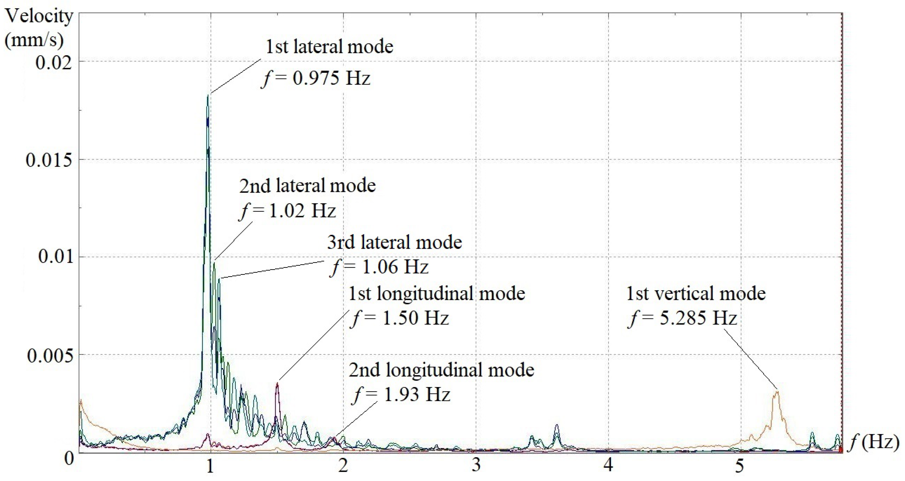
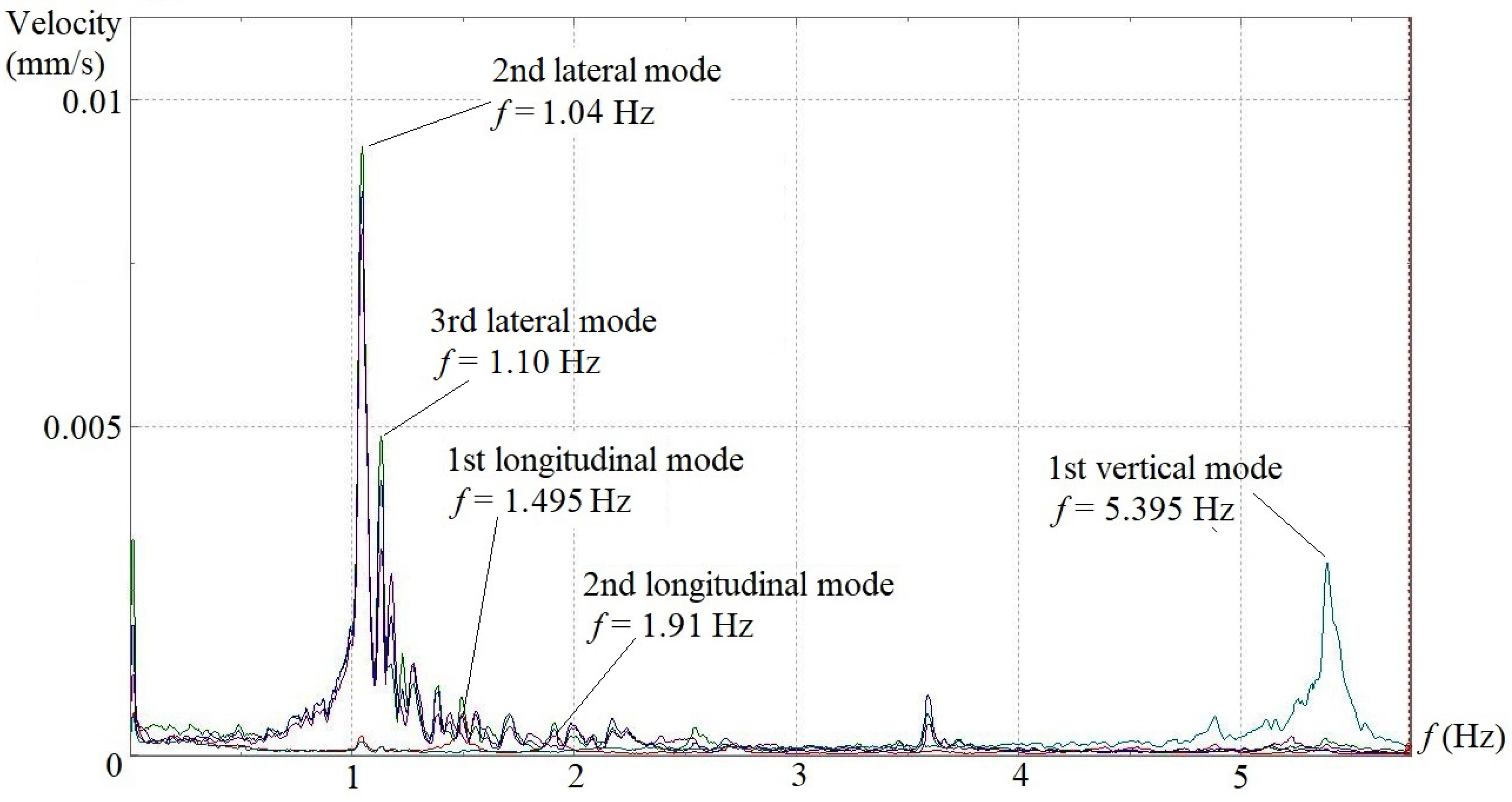
It is obvious that the lateral vibration of the aqueduct is dominant among three directions, with its velocity amplitudes being higher than those along the longitudinal and vertical directions. Span 6 and span 8 essentially demonstrate the same lateral vibration feature in which the frequencies of the first, second and third lateral modes stand at 0.97~0.975 Hz, 1.02 Hz and 1.06 Hz, respectively, and the first mode has much higher velocity amplitude than the other two. Span 10 has the same lateral mode frequencies with span 6 and span 8, but contrary to the two former spans, the velocity amplitude of the first mode is lower than those of the second and third modes. Span 14 does not show the first lateral mode at 0.97 Hz on the velocity spectrum, but two other peak amplitudes appear at 1.04 Hz and 1.10 Hz, which are quite close to the second and third lateral modes of the other three spans. Although the four sets of results cannot be compared with one another directly since dynamic tests were conducted individually for each span, a general trend can still be observed that the lateral velocity amplitudes of span 6 and span 8 are much higher than those corresponding values of span 10 and span 14.
The longitudinal vibration of the aqueduct basically exhibits two main modes on the four velocity spectra. The frequencies of the first longitudinal modes locate consistently at 1.495~1.50 Hz, while the second longitudinal modes fluctuate within a very small range of 1.885~1.935 Hz. Unlike the lateral and longitudinal vibrations, the vertical vibration of the aqueduct only manifests a single peak frequency around 5.285~5.395 Hz on the velocity spectra of all four spans, with the velocity amplitudes maintaining at almost the same magnitude.
From those field test findings, the dynamic characteristics of the whole aqueduct can be summarized in
Table 1.
3. Modal Analysis of the 3D Aqueduct Model
A 3D FE model is established using SAP2000 for the entire aqueduct, as shown in
Figure 2. The arch trusses, transverse bent frames above those trusses, moment frame supports and foundation piles are generated by frame elements, and the water-transferring U-shaped flumes and pile foundation caps are created using shell elements. A 3 cm-wide contraction joint is set between two adjacent U-shaped flume segments. The pot-type fixed rubber bearing of the arch trusses at the upstream end of each span is simulated as a rubber isolator restrained in all translational and rotational DOFs, while the pot-type sliding counterpart at the downstream end of each span is modeled with the same DOF restraints except that the shear stiffness in the longitudinal translation is set to be zero.
The interaction between foundation piles and surrounding soil is simulated with node springs using “m” method. According to the current Chinese code “Technical Code for Building Pile Foundations (JGJ 94-2008) [
26]”, the lateral stiffness of the node spring of a pile can be calculated as follows:
where
K is the lateral stiffness of the node spring (kN/m);
a is the thickness of the foundation soil layer, normally taken as 1~2 m;
b0 is the effective width of the pile (m), and when the pile diameter
d is larger than 1 m,
b0 = 0.9 × (
d + 1); Z is the depth of the foundation soil layer (m); and
m represents the proportional coefficient of horizontal resistance of foundation soil (kN/m
4), and for cast-in-place concrete piles can be taken as shown in
Table 2 for different foundation soils (in this case, it can be taken as 100~300 MN/m
4).
In the real structure, the prefabricated U-shaped concrete flume segments are laid directly on the top beams of transverse bent frames erected on the arch trusses, but the bearings only adopt two layers of thin (about 1 mm thickness) asphaltic felts instead of commonly used plate rubber supports. In the 3D model, this makeshift asphaltic bearing is simulated by an elastic link element restrained in vertical translation and rotation about the vertical axis while free in the other two rotational DOFs, but the shear stiffnesses in the transverse and longitudinal directions need to be defined, which can be assumed to be equal based on the empirical equation:
where
K is the bearing shear stiffness,
G is the shear modulus of the bearing material,
A is the plane area of the bearing, and
t is the bearing thickness.
The influence of the “m” value variation of foundation soil on the dynamic characteristics of the aqueduct was investigated. In this case, certain dynamic elastic moduli are assumed for arch trusses (40 GPa), bent frames (37.5 GPa), moment frame supports (37.5 GPa), pile caps and piles (32.5 GPa) in the 3D model based on their respective design strengths, and the shear stiffnesses of asphaltic bearings of U-shaped flumes in both transverse and longitudinal directions are set to be 1.536 × 10
7 kN/m. The modal analysis results are listed in
Table 3. It can be seen that the change of the “m” value in a code-specified range has an insignificant impact on the dynamic characteristics of the aqueduct.
By altering one of those parameters while keeping others unchanged, the sensitivity analyses of dynamic elastic moduli of arch trusses (
Ed-arch), bent frames, moment frame supports (
Ed-frame), pile caps and piles (
Ed-pile) on the dynamic characteristics of the aqueduct are conducted, and the results are shown in
Table 4,
Table 5 and
Table 6. It can be seen that under almost the same variation,
Ed-pile has much less influence compared with
Ed-arch and
Ed-frame, which may be attributed to the large rigidity of the foundation (i.e., pile cap thickness 1.5 m and pile diameter 1.5 m). It is also found that the vertical frequency is sensitive to
Ed-arch, while the lateral and longitudinal frequencies are sensitive to
Ed-frame.
The flumes have the same design strength (C40) with bent frames and moment frame supports, so in the modal analysis, the dynamic elastic modulus
Ed-flume is assigned to be the same with
Ed-frame. Following the same procedure, the impact of
Ed-flume variation on the dynamic characteristics of the aqueduct was also investigated and found to be minor, as shown in
Table 7.
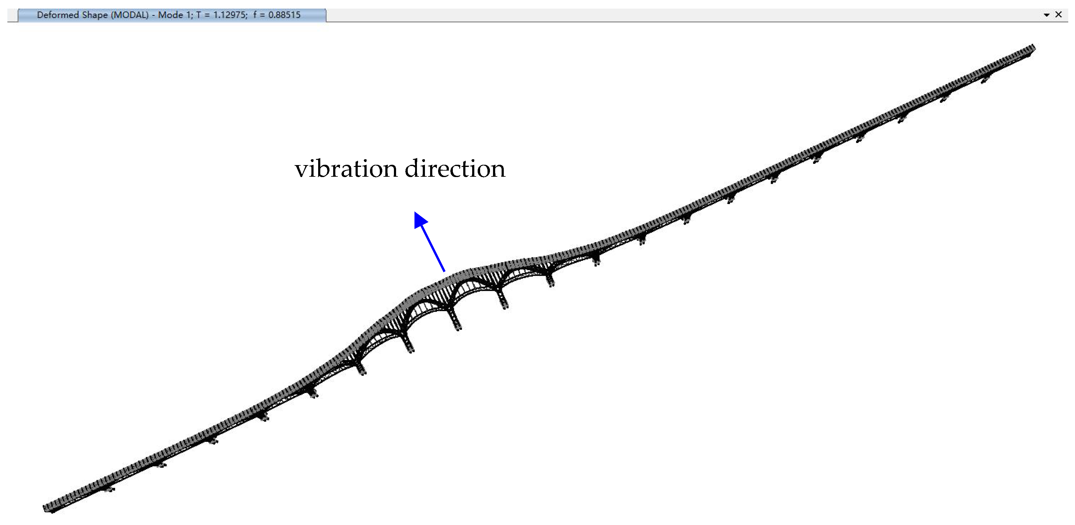
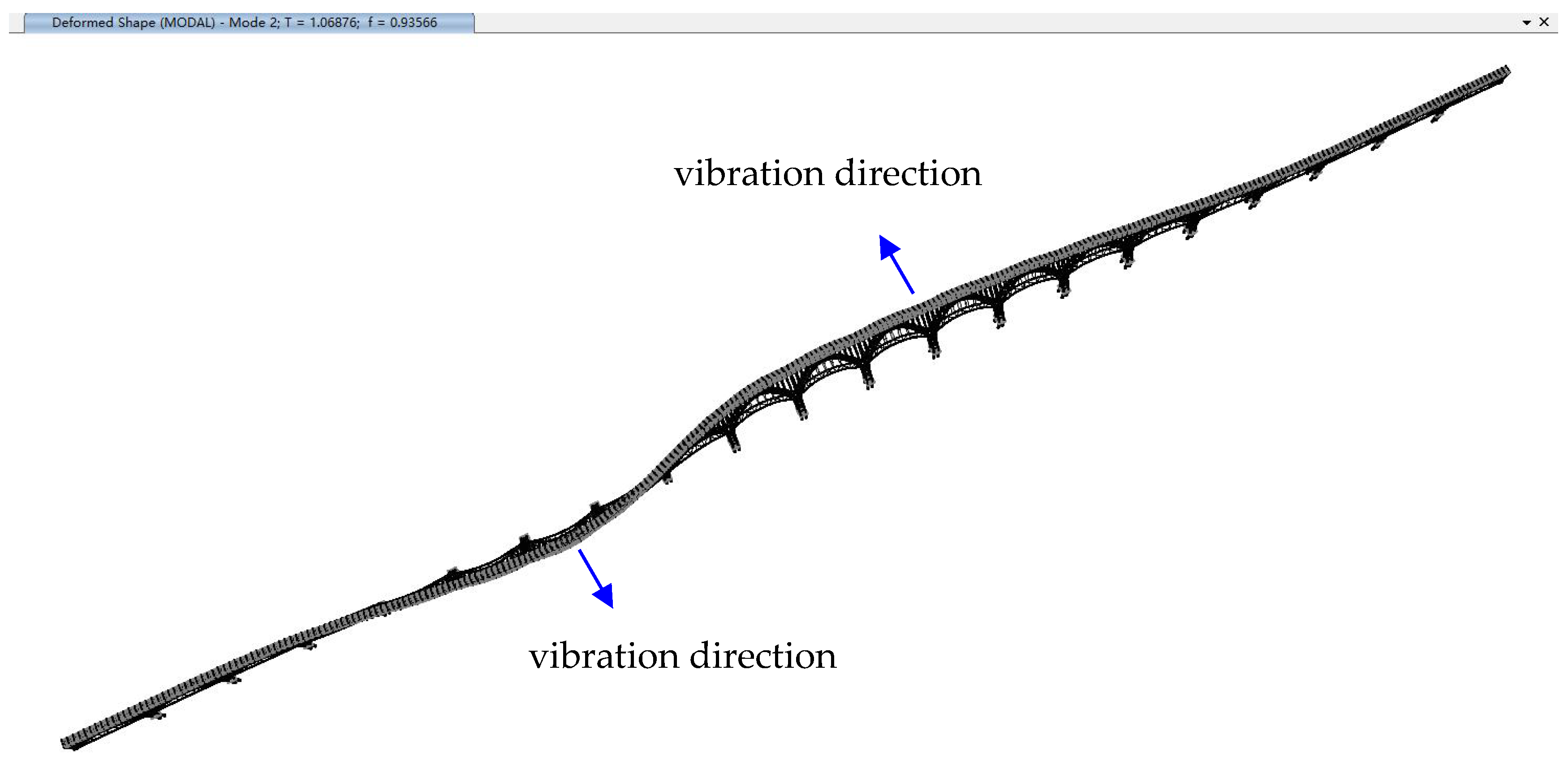
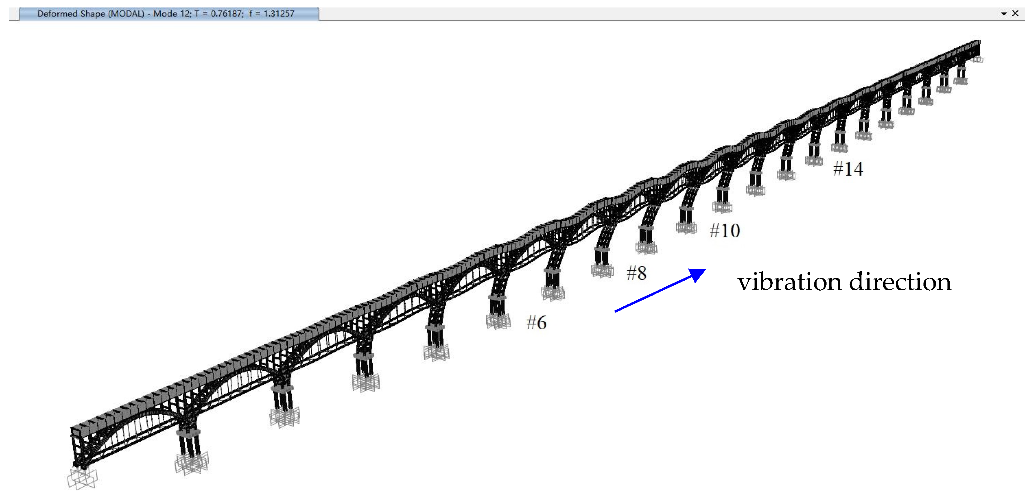
Therefore, after neglecting those two parameters, the main parameters left that may affect the dynamic characteristics of the 3D aqueduct model are the shear stiffnesses of the asphaltic bearings of U-shaped flumes, the dynamic elastic modulus of arch trusses (concrete design strength C50), and the dynamic elastic modulus of bent frames and moment frame supports (C40). By arranging those 3 parameters into various combinations, a series of modal analyses of the aqueduct are performed, and the typical primary mode shapes are shown in
Figure 10,
Figure 11,
Figure 12,
Figure 13,
Figure 14 and
Figure 15.
The first lateral modes of the aqueduct for all analysis scenarios have modal participating mass ratios nearing 20%, which are higher than those of other lateral modes. As shown in
Figure 10, the first lateral mode typically manifests itself as a lateral vibration of some interior spans (i.e., span 6 to span 11) in the same direction, whereas the motions of exterior spans including span 14 are not activated, which may justify the missing of the first lateral mode on the velocity spectrum of span 14 (see
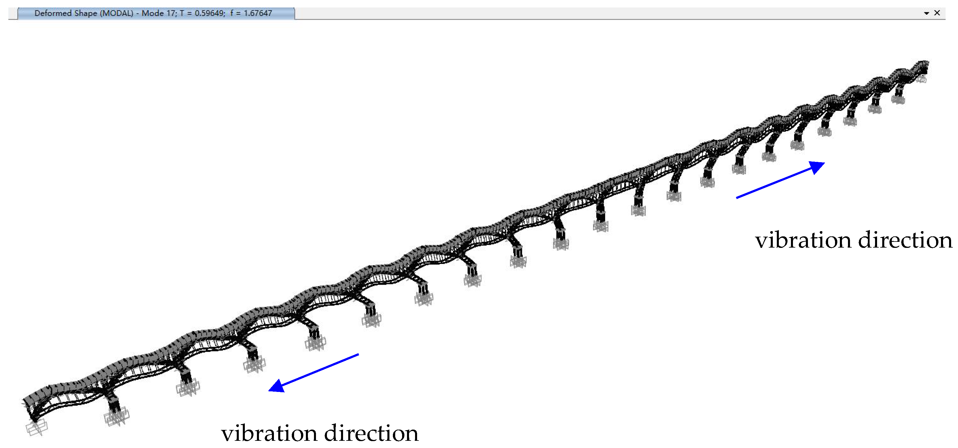
Figure 7). It can be seen from
Figure 11 and
Figure 12 that the second and third lateral modes involve transverse vibration of more spans including span 6, 8, 10 and 14, which conforms to the appearances of these two modes on all velocity spectra obtained from field dynamic tests (see
Figure 4,
Figure 5,
Figure 6 and
Figure 7).
As shown in
Figure 13 and
Figure 14, the first (normally with a modal participating mass ratio around 20~50%) and second longitudinal modes of the aqueduct for all analysis scenarios both show longitudinal vibration of most spans concurrently, which also accords with the presence of two longitudinal peak frequencies in
Figure 4,
Figure 5,
Figure 6 and
Figure 7.
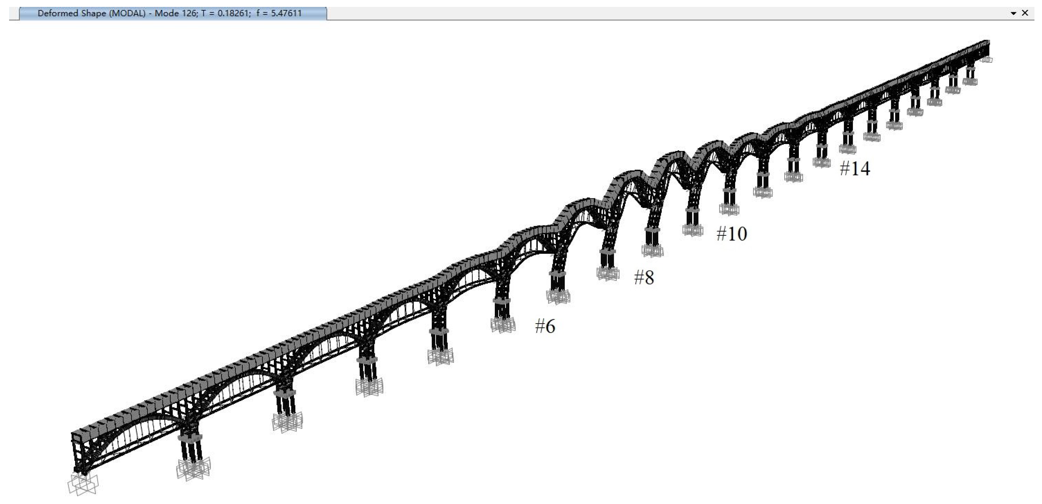
The first vertical modes of the aqueduct for all analysis scenarios have modal participating mass ratios around 20%, typically displaying a simultaneous vertical vibration shape of arch trusses in most interior spans, as shown in
Figure 15. In fact, there still exist one or two similar vertical modes which have slightly lower or higher frequencies but much less modal participation mass ratios than that primary mode, and this may explain the small differences of the first vertical mode frequencies obtained from the field dynamic tests of the four spans, as shown in
Figure 4,
Figure 5,
Figure 6 and
Figure 7.
4. BP NEURAL Network Modeling
As discussed in
Section 3, each combination of shear stiffnesses of the asphaltic bearings of U-shaped flumes (
Kflume), the dynamic elastic modulus of arch trusses (
Ed-arch) and the dynamic elastic modulus of bent frames and moment frame supports (
Ed-frame) will yield a set of primary modal frequencies of the aqueduct in three directions. So, according to the Universal Approximation Theorem of a feed-forward neural network [
27],
Kflume,
Ed-arch and
Ed-frame of the aqueduct can be approximated with a BP neural network using the primary modal frequencies of the structure obtained from the in situ dynamic tests.
To fulfill the BP neural network modeling, a large number of modal analyses of the 3D aqueduct model need to be conducted to obtain the training data.
Using Equation (2), for a rubber bearing with A and t being 250 × 400 mm2 and 2.0 mm, respectively, the shear modulus G can be taken as 1.2 MPa per the Chinese code “Laminated Bearing for Highway Bridge (JT/T 4-2019)”, and then the bearing shear stiffness would be calculated as 6 × 10⁴ kN/m. However, the asphaltic bearing material is not rubber, and its mechanical property is difficult to determine. Taking the hardened asphalt as a reference, the elastic modulus typically falls into a range from 1000 MPa to 9000 MPa, so the bearing shear stiffness could be several thousand times the rubber bearing. Considering other unknown factors, Kflume array is then formed using a geometric progression in a wide range from 4.8 × 10⁵ kN/m to 1.2288 × 10⁸ kN/m with a constant multiplier of 2, which contains 9 elements. Ed-arch and Ed-frame are taken from two arithmetic progressions from 35 GPa to 60 GPa and from 30 GPa to 55 GPa with a constant increment of 5, respectively, and 20 pairs are randomly selected. Each pair of Ed-arch and Ed-frame is combined with each element of the Kflume array, which leads to a total of 180 combinations.
These 180 combinations of Kflume, Ed-arch and Ed-frame are put back into the 3D model individually to perform modal analyses, while the “m” value of foundation soil and the dynamic elastic modulus of pile caps and piles are taken as constant values (300 MN/m4 and 35 GPa, respectively). Each combination will generate one set of primary modal frequencies of the aqueduct (i.e., the first, second and third lateral modes fT1, fT2 and fT3, the first and second longitudinal modes fL1 and fL2, and the first vertical mode fV1,), which finally creates a dataset with 180 lines, and each line contains 9 elements, namely, the six inputs fT1, fT2, fT3, fL1, fL2, fV1 and three outputs Kflume, Ed-arch, Ed-frame.
In BP modeling, this total dataset is randomly divided into training, validation and testing sets with a division ratio of 8:1:1, so the sizes for the three sets are 144, 18 and 18, respectively. The validation set is employed to optimize the hyperparameters of the BP neural network (i.e., the number of hidden layers, the size of each hidden layer and the transfer function of each layer). Since the size of the training and validation dataset (180) is relatively small, a K-fold cross-validation process is utilized with K = 9. So, the BP neural network will be trained 9 times, and the average MSE (mean square error) and the average MAE (mean absolute relative error) of the 9 validations will be used to determine the optimal architecture of the network.
Since the ratio of the minimum input
Kflume to its maximum value is only 1/256, it is found in the BP neural network pretraining that approximations are not satisfactory. So,
Kflume in the total dataset is pretreated with natural logarithm, but even after this pretreatment, a BP neural network with just one hidden layer still gives rise to notable errors through the aforementioned 9-fold cross-validation process. So, a BP neural network with two hidden layers is employed, and when the neuron number for each hidden layer is 9, the cross-validation results for the transfer functions of the hidden and output layers are shown in
Table 8, where case 6 gives the best approximation and quick convergence. Further investigation shows that when the neuron number of each hidden layer is decreased to 7 or increased to 11, the average MAE and MSE will not show any improvement.
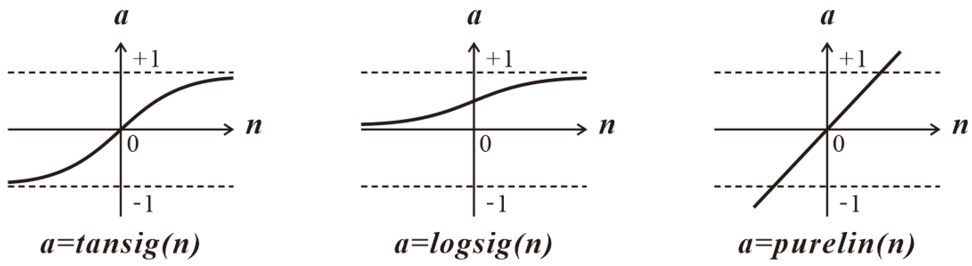
MATLAB is used to perform the BP neural network modeling and approximation. The purelin, tansig and logsig transfer functions are illustrated as shown in
Figure 16:
Therefore, it can be concluded that a BP neural network of which both the first and second hidden layers have 9 neurons with a transfer function of “logsig” and the output layer has 3 neurons with a transfer function of “tansig” can provide very good approximations for
Kflume,
Ed-arch and
Ed-frame. The final BP neural network for evaluating
Kflume,
Ed-arch and
Ed-frame is trained using this architecture with the training and validation dataset, and then the testing dataset is applied, which produces the following test results, as shown in
Table 9.
Using the dynamic characteristics of the whole aqueduct obtained from field tests, as shown in
Table 1, as the six inputs (
fT1 0.97 Hz,
fT2 1.02 Hz,
fT3 1.06 Hz,
fL1 1.50 Hz,
fL2 1.915 Hz and
fV1 5.328 Hz) of the trained BP neural network, the three outputs (
Kflume,
Ed-arch and
Ed-frame) are estimated to be 1.2288 × 10
8 kN/m, 47.8 GPa and 46.1 GPa, respectively. It should be noted that
Kflume is approximated to be the maximum value of the corresponding training data, and this indicates that the asphaltic bearings of U-shaped flumes essentially behave more like a three-directional hinge which cannot provide effective dynamic isolation during seismic events.
Normally the first modes of the aqueduct in three directions are most prone to be excited when the structure is subjected to exterior dynamic loading, so technically they can be more easily and accurately detected by a field dynamic test than the other higher modes. If only such three frequencies as
fT1,
fL1 and
fV1 are chosen as the inputs of the BP neural network of which the architecture still adopts the one specified by case 6 in
Table 8, the modeling results of
Kflume,
Ed-arch and
Ed-frame using the same training and test procedures for
Table 9 are shown in
Table 10. It can be seen that a BP neural network with only 3 inputs (
fT1,
fL1 and
fV1) is still capable of providing good approximations for
Kflume,
Ed-arch and
Ed-frame. By substituting the three first modes of the aqueduct in three directions (
fT1 0.97 Hz,
fL1 1.50 Hz and
fV1 5.328 Hz) into the BP neural network specified in
Table 10, the three outputs (
Kflume,
Ed-arch and
Ed-frame) are estimated to be 1.2288 × 10
8 kN/m, 48.1 GPa and 44.3 GPa, respectively. It can be seen that the BP neural networks with six and three inputs generate almost the same approximations for
Kflume and
Ed-arch, but the approximations for
Ed-frame are somewhat different.
To evaluate which network could provide a better prediction, the three outputs (
Kflume,
Ed-arch and
Ed-frame) obtained from those two BP neural networks are fed back into the 3D FE model to perform the modal analysis, and the results are shown in
Table 11 and
Table 12.
It can be seen that the FE modal analysis using Kflume, Ed-arch and Ed-frame predicted by the BP neural network with six inputs generally show improved approximations to the main modal frequencies obtained from the in situ dynamic tests, especially for fL1 and fL2, indicating that more input information on modal frequencies could enhance the prediction accuracy of the BP neural network.
5. Conclusions
For the aqueduct under investigation in this study, Kflume, Ed-arch and Ed-frame are among the main parameters to define its dynamic behavior, but there is no easy approach to get them tested directly on site. Since these parameters have direct correlation with the vibrational characteristics of the aqueduct, it is practicable to apply a BP neural network to evaluate them using the primary modal frequencies of the structure as inputs. However, it is impossible to obtain a large amount of experimental data to train the network from the real structure. To solve this data deficiency problem, a full-scale 3D FE model which can simulate the real structure to its best is established, and various modal analyses under different combinations of Kflume, Ed-arch and Ed-frame are conducted to create the analytical dataset for the network. Through cross-validation procedure, the network architecture with two hidden layers is determined, and it shows that with appropriated transfer functions for the hidden and output layers, the trained BP neural network can provide very good approximations for Kflume, Ed-arch and Ed-frame using the primary modal frequencies obtained from the FE model.
The actual primary modal frequencies acquired from in situ dynamic tests are then put into the BP neural network to estimate Kflume, Ed-arch and Ed-frame of the aqueduct. By substituting the Kflume, Ed-arch and Ed-frame obtained from two BP neural networks with different sizes (6 and 3) of input frequency vectors into the 3D FE model, it is found that more inputs of modal frequencies can improve the approximation accuracy of the BP neural network.
Finally the Ed-arch and Ed-frame of the aqueduct are approximated to be 47.8 GPa and 46.1 GPa, respectively, and Kflume is estimated to be the maximum value of the corresponding training data, implying that the makeshift asphaltic bearings of U-shaped flumes basically can be treated as a three-directional hinge (i.e., fixed in vertical, lateral and longitudinal translations) in the FE model.


