Abstract
The utilization of low-cost AGVs in the industry is increasing every day, but the efficiency of these systems is low due to the lack of a central management system. Low-cost AGVs’ main characteristic is navigation via magnetic sensors, which they follow via magnetic tape on the ground with a low-level automation system. The disadvantages of these systems are mainly due to only one circuit assignment and the lack of system intelligence. Therefore, in this study, AGV pools were employed to determine the required AGV number. This study begins by calculating the required AGV number for each AGV circuit combination assigned to every parking station by the time window approach. Mathematical-solution-based mixed integer programming was developed to find the optimum solution. Computational difficulties were handled with the development of a genetic-algorithm-based approach to find the solutions for complex cases. If production requirements change, system parameters can be changed to adapt to the production requirements and there is a need to determine the number of AGVs. It was demonstrated that AGVs and pool combinations did not lead to any loss in production due to the lack of available AGVs. It was shown that the proposed approach provides a fleet size which requires five fewer AGVs, with a 29% reduction in the number of AGVs. The effects of system parameter changes were also investigated with artificial neural networks (ANNs) to estimate the required AGVs in the case of production requirement changes. It is necessary to determine the effect of the change in system parameters on the number of AGVs without compromising on computational cost and time, especially for complex systems. Thus, in this study, an artificial neural network (ANN), the response surface method (RSM), and multiple linear regression (MLR) techniques were used to examine the effects of the system parameter changes on the AGV number. In the present case, the ANN obtained the solution at a good rate with reduced computational costs, time, and correction errors compared to the GA, at 0.4% (ANN), 7% (RSM), and 24% (MLR). The results show that the ANN provides solutions which can be used in workshops to determine the number of AGVs and also to predict the effect of changes in system parameters.
1. Introduction
Automated guided vehicles (AGVs) are capable of automatic material transportation without the need for a driver. AGVs are employed in manufacturing and service industries, including automobile production plants, semiconductor manufacturing workshops, flexible manufacturing systems (FMSs), seaport container terminals, and the health sector [1,2,3]. Material handling has a significant impact on production costs in every production activity [4]. In Industry 4.0, AGVs are an indispensable solution and AGV developers must find solutions to customer-specific and personalized demands, but solutions must fulfil economic expectations [5,6,7]. Employment of AGVs is a capital investment that requires analysis of station locations, optimal route design, determination of the optimal number of AGVs and types, AGV positioning, assignment of the AGVs to collection requests, AGV routing and dispatch, resolving deadlocks and conflicts, scheduling and determination of the capacity, and other factors. The AGV fleet size has a significant impact on the work conditions of AGVs and the economy of AGV installation and implementation [8,9,10].
High investment costs force companies to adopt low-cost AGV solutions. Utilization of low-cost AGVs in industry is increasing every day, but the efficiency of these systems is low due to the lack of a central management system [11,12]. Although various numerical and experimental studies have previously been conducted, the problem of grouping AGV circuits and AGV assignments to parking stations to minimize the number of AGVs while meeting demand is still being researched in the field of manufacturing.
Low-cost AGVs’ main characteristic is navigation via magnetic sensors, which they follow by magnetic tape on the ground, and they require a low level of automation, so they include a PLC or an embedded system [13]. These systems lack central control systems. A centralized control system manages all AGVs, but it has some drawbacks mainly due to the expensive cost, lack of flexibility, robustness, and scalability [11]. Therefore, decentralized solutions are attracting attention in industry. On the other hand, low-cost AGVs are assigned to a single AGV path, resulting in a low AGV efficiency. They reduce the AGV cost, but growing the AGV fleet does not create an optimum investment cost. All AGV circuits contain a waiting time, and if this time cannot be used for another part transfer, the AGV will remain in a waiting state, which will cause the efficiency of the AGV to decrease. Creating an AGV pool also makes use of these waiting times. The aim of this research is to determine the optimum number of AGVs for decentralized low-cost AGV systems and also to examine the effect of the change in system parameters on the required number of AGVs when a change in production requirements is necessary.
This study begins by calculating the required AGV number for each AGV circuit combination assigned to every parking station by the time window approach with a developed algorithm. To determine the best solution, a mathematical model is presented to determine the minimum number of AGVs for one or multiple automated guided vehicle pools. The analytical mixed integer linear programming (MILP) method was introduced to achieve an optimal solution. Mathematical-solution-based mixed integer programming provides the optimum solution [14]. It was observed that the variables increased exponentially with the number of AGV circuits, reducing the utility of the model in complex applications. It becomes more complex with the increase in the number of stations. It is very difficult to implement the MILP approach in complex problems since it takes time to determine the equations and build the model for a particular problem. The problem turned in to an NP hard problem. Thus, a heuristic genetic algorithm was proposed to determine the number of AGVs with time windows for further complex situations. The present approach was employed in a workshop and the solutions were validated through discrete event simulation in the Witness program [15].
In workshops, production requirements may change. If production requirements change, system parameters can be changed to adapt to production requirements. There is a need to examine the required number of AGVs by estimating the effect of the change in system parameters without compromising on computational cost and time. Therefore, an artificial neural network was employed to estimate the number of required AGVs assigned to AGV circuits and to parking stations. Artificial neural network (ANN), response surface method (RSM) and multiple linear regression (MLR) techniques were used to investigate the effects of the system parameter changes on the required AGV number. A comparison of these techniques was implemented to find the most effective technique to examine the effects of the system parameter changes on the required AGV number. The results show that ANN-estimated solutions are in good correlation and can be used in workshops.
2. Literature Review
In the literature, several studies have approached AGVs and AGV systems from various perspectives. Vis (2006) reviewed the existing methods in the literature and reported that models developed to design and control AGV systems could overcome certain problems, but new approaches were required to overcome long computation times and other problems such as congestion, deadlock, and delays in extensive AGV systems [16].
An AGV moves on a path which is fixed or variable depending on the AGV type. The path assignments affect the number of AGVs. Soylu et al. proposed the employment of an artificial neural network to determine the shortest path for a single AGV. It was aimed to determine the minimum total empty travel time. Good findings were reported for computation time. Although the algorithm achieved acceptable solutions, none of them were optimal or near optimal in certain sequential models [17]. In another work, the AGV path was analyzed with the Ant Colony Optimization (ACO) algorithm, and it was demonstrated that the route determined with ACO improved the efficiency within an acceptable time [18]. Bozorgi-Amiri et al. proposed a split delivery vehicle routing problem to minimize vehicle travel on a path. They compared memetic heuristic and mathematical models [19].
The management of AGV traffic is another significant problem. Traffic management entails the prevention of collisions and deadlocks that could block the AGV system. Management could be conducted with a central control system or various routing methods. Nishi et al. (2007) proposed a decomposition method with a cut generation to efficiently solve collisions or deadlocks across AGVs [20]. Rocak et al. presented a dynamic routing method for multiple AGVs with time windows. In the case of a collision on the selected route at a specific time, the algorithm looks for another route. The efficiency of the method was demonstrated by simulation [21]. Cardarelli et al. suggested the use of real-time AGV and route monitoring, which allowed the system to run AGVs online and avoid problems such as deadlocks [22]. Parham suggested the employment of new-generation AGVs during deadlocks that would allow θ° around the center of a circle, and after the transition, the AGV would return to its original position [23]. Hsueh proposed a system where the AGV could change its load in the case of a deadlock. These studies improved AGV system flexibility, albeit by increasing the AGV cost, while maintenance problems negatively affected the system performance [24].
Routing strategies and rules affect the number of AGVs in the system, as well as other factors such as the Pick & Deposit (P&D) location. Vehicle requirements entail the number of AGVs required to fulfill system transport demands. This issue is also known as fleet sizing. According to Vis, the fleet is sized based on transport load demands, time demands, AGV capacity, AGV speed, routing, traffic management, AGV assignment, and P&D locations [16]. Ventura and Lee emphasized the response time as a factor in fleet size calculations. The response time is the idle travel time until the next pickup. They tried to minimize the reaction time [25]. The minimization of this non-value-added time would reduce the total transport time. The minimization of the maximum response time with positioned waiting points in an AGV system was analyzed by Ventura et al. to minimize the average response time. A single loop pattern was analyzed and compared with the mathematical model and genetic algorithm approach, and the authors observed that the computation time increased with the model size and the GA could be optimized with the mathematical model [26].
Nishi et al. proposed a distributed routing method with motion delay disorder to minimize the transport time with multiple AGVs, which reduced the collision probability and collision-related penalties. The findings demonstrated that the proposed method could be implemented in real transportation environments [27]. Talbot developed and investigated a queuing model to estimate AGV fleet sizes; however, the model produced inferior solutions in light traffic [28].
Simulation techniques are frequently employed in the search for solutions to problems associated with AGVs [2]. Valmiki et al. estimated the AGV fleet size in a simulation based on minimizing the total travel time and total cost. It was reported that the simulation method provided an accurate fleet sizing solution when compared to the analytical method [29]. Viharos et al. proposed a simulation model to control the AGVs. A methodology based on shortening the total operational manufacturing time was proposed [30]. In another approach, Yifei et al. reported that it could be difficult to assign an accurate number of AGVs with the mathematical model and it could take time to simulate the entire system. In the first stage, they estimated the required number of AGVs with the mathematical model and reduced the computation time, since they utilized the output as the simulation input. They reported that the fleet size estimation for multi-loaded AGVs with the heuristic method was not accurate when compared to real- life requirements; however, simulation methods led to a better solution [31].
Şenaras analyzed AGV parameters with the surface response and simulation method to determine the optimal parameters to minimize the required number of AGVs [32].
Chang et al. applied simulation optimization and data envelopment for multi-objective (minimum delivery time and maximum lot delivery) vehicle fleet sizing in an automated material handling system. The numerical study demonstrated that the proposed method provided accurate solutions [33]. Rashidi et al. proposed a minimum-cost flow model for container terminals. A simplex algorithm and greedy search method were adopted to solve the model. They demonstrated that the time-constrained greedy tool search could complement the simplex algorithm, which requires further computation time. The AGV simplex model provided the optimal planning solution; however, as the number of work orders increased, the computation time forced the analyst to convert to the greedy algorithm. However, this algorithm could not always determine the optimum solution and got stuck at the local minimum [34].
Saidi-Mehrabad et al. proposed a model that included a workshop scheduling problem and a conflict-free routing problem and utilized Ant Colony Optimization (ACO) to minimize the AGV production time and guide the AGVs to avoid collisions. A mathematical method and an ACO model were developed. It was suggested that the ACO model could reduce the computation time [35]. The same topic was studied by Nishi et al. (2007), who suggested the employment of a bilevel decomposition algorithm to solve simultaneous scheduling and conflict-free routing problems and minimize the total weighted tardiness of the task sets. Lagrangian relaxation reduced the computation time, which was an important issue in higher task counts [36]. The decomposition method has been frequently used in scheduling and routing. Nishi et al. developed an AGV routing solution with a Petri net by decomposing the problem into sub-problems that were solved with Dijkstra’s algorithm [37].
Several cut methods, as well as heuristic methods, were studied to solve sub-problems. Moghaddam et al. proposed an advanced particle swarm optimization algorithm for vehicle routing problems under uncertain customer demand. The novel method was reported to improve the solution quality and the algorithm was determined as adequate for large-scale problems [38].
Another study was conducted with robust vehicle routing optimization under uncertain demand by Moghadam et al. The application of robust optimization in vehicle routing problems under uncertain demand reduced the unmet demand [39].
Fazlollahtabar proposed the employment of a scheduler to assign AGVs and machines in the short term and a heuristic model was developed for this assignment. The proposed framework included a two-level hierarchical dynamic decision for AGV dispatch and selection of the next station based on the minimum cost flow, a machining scheduler, and a station controller for operation control. The findings revealed the effectiveness of the dispatch rule by decreasing the average flow time. Artificial intelligence and bi-level programming could be investigated in a future study [40]. This study was conducted with online scheduling, while other studies employed offline scheduling. Lacomme et al. studied offline AGV and machine scheduling and proposed a framework based on a disjunctive graph to model the common schedule problems and a memetic algorithm to schedule the machines and AGVs. The aim was to minimize the production time. A comparison of the results demonstrated that the proposed algorithm could provide optimal solutions to schedule machines and AGVs concurrently [41].
H. F. Rahman et al. investigated robot line balancing and AGV scheduling with a two-stage heuristic approach to assist the manager to develop or modify an effective robot line. In the first stage, the consecutive algorithm is employed to balance the robot assembly line, and in the second phase, Particle Swarm Optimization (PSO) was used to schedule AGVs between robot stations [42]. Digital-twin-based solutions have also been used for AGV scheduling. The battery charging problem was investigated with this method and a 1.32% energy saving was obtained [43]. Kim and Park tested various vehicle circulation rules to minimize the average lead time. A simulation demonstrated the effect of the rules on system effectiveness [44]. Generally, the dispatch and routing problem tackles the problem of incapacitated AGVs. Miyamoto et al. employed the integer model to dispatch capacitated AGV systems. First, the mathematical solution was studied, then local search and random search methods were tested, and it was reported that the local search algorithm led to a better solution for the large-scale problem [45].
Although various numerical and experimental studies have previously been conducted, the problem of grouping AGV circuits and AGV assignment to parking stations to minimize the number of AGVs while meeting the demand is still being researched in the field of manufacturing. Several studies have been conducted on the design and control of AGV systems; these were mostly based on computer-assisted high-cost AGV systems. Considering low-cost AGVs, determination of the minimum fleet size by creating AGV pools via time windows and examinations of the effects of the system parameter changes on the required AGV number using ANNs if the production requirements change have not been widely investigated in the literature.
3. State of the Problem
AGV systems include vehicles, control systems, and peripheral components. Depending on the selection of AGV systems, the investment is a major barrier for companies. Therefore, utilization of low-cost AGVs in the industry is increasing every day [7,13].
Generally, low-cost AGVs follow magnetic tape on the ground and contain a PLC as a controller. With the removal of the central control system, the AGV system evolves into vehicles operating between a single production station (where the product is fabricated) and a single consumption station (where the product is used), as shown in Figure 1. The production station and the associated consumption station form an AGV circuit.
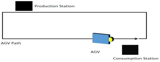
Figure 1.
AGV single circuit illustration.
The application of low-cost AGVs led to a less flexible system and difficulties in changing the AGV path. As a result, this type of AGV operates with a low usage rate due to waiting for production stations. The inclusion of decentralized control systems allows the formation of AGV pools, where the AGV can service various AGV circuits. AGV programs can be changed in a Parking Station, where a decentralized control device can communicate via an optical device and change the AGVs’ program, as shown in Figure 2.
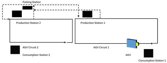
Figure 2.
AGV multi-circuit illustration.
The problem turns into grouping the AGV circuits using AGV pools and assigning these combinations to parking stations to achieve a minimal AGV fleet size while meeting the production demand.
3.1. Determination of the Required Number of AGVs
In this study, the problem is the determination of the number of AGVs and the effect of the change of system parameters on the number of AGVs for low-cost AGV systems. This study was presented in two stages. In the first stage, the proposed approach starts by calculating the required AGV number for each AGV circuit combination assigned to every parking station by time window and obtains the optimum AGV fleet size. The second stage is concerned with examining the number of AGVs after the change in system parameters if the production requirements change.
The developed mathematical-solution-based mixed integer programming provides the optimum solution for the simple case. However, the problem becomes more complex with the increase in AGV circuits. Since the mathematical model cannot solve large-sized complex problems, GA is proposed to handle this type of problem. Computational difficulties make it necessary to develop a genetic-algorithm-based approach to obtain solutions for complex cases. Finally, an artificial neural network (ANN) was employed to investigate the effects of the system parameter changes on the required AGV number.
3.2. Time Window Approach
In the first stage, the required AGV number was computed for each AGV circuit combination assigned to every parking station by the time window approach. The time windows are from the beginning of the allowable service time (a) to the end of the allowable service time (b) for each order. Each order should be fulfilled within these time intervals. The parameters and notations used in this problem and their explanations are given in Table 1.

Table 1.
The parameters and notations of the problem.
An AGV cannot deliver the parts before the beginning and after the end of the allowable service time. (1) The release time of AGV k is calculated by adding an assignment of time to the time required to finish a tour. (2) The first order (O = 1) is realized with the first AGV (k = 1). If the above constraints are not satisfied with the current number of AGVs, the required number of AGVs is increased by 1, otherwise k remains constant. This approach can easily produce a solution for low order numbers and AGV circuit combinations, but if the complexity of the system increases, it needs to be solved with an algorithm, since the number of calculations increases exponentially with the number of AGV circuits. The algorithm first checks the AGV transfer order. If the AGV request is associated with this AGV circuit combination, the request is assigned to the first AGV (k = 1) and the release time of the AGV is calculated. When a new request arrives, the algorithm checks if there is an idle AGV. If there is an AGV available, this AGV is assigned to the new order; however, if an AGV is not available, an additional AGV is added to the system to meet the new request. This algorithm was run on Matlab R17 for all AGV line combinations and all parking stations [46]. The pseudocode for this algorithm is shown in Algorithm 1.
| Algorithm 1: Compute the required number of AGVs for each station combinations and each parking stations |
| 1 Initialize |
| 2 WHILE stop condition not fulfilled DO |
| 3 Begin |
| 4 FOR parking station: =1 TO I DO |
| 5 FOR station combination: = 1 TO B DO |
| 6 Assigned = 0 |
| 7 Used = 0 |
| 8 FOR order: =1 TO O DO |
| 9 FOR station combination index: =1 TO S DO |
| 10 IF order station == station combination index THEN |
| 11 Find min agv release time, define as miniagv and agv row as miniindex agv |
| 12 IF miniagv < aj THEN |
| 13 Assigned = miniindex agv |
| 14 fok = a j |
| 15 eok = fok + ts |
| 16 Else IF aj < miniagv < bj THEN |
| 17 fok = miniagv |
| 18 eok = fok + ts |
| 19 Else IF bj < miniagv THEN |
| 20 Used = Used + 1 |
| 21 Assigned = Used |
| 22 fok = aj |
| 23 eok = fok + ts Set of combinations for the sth AGV circuit sÎS |
| 24 END |
| 25 END |
| 26 Usedagv(parking station, station combination) = Used |
| 27 END |
| 28 END |
3.3. Mathematical Model and Optimization
In this stage, mathematical-solution-based mixed integer programming provides the optimum solution. Linear programing consists of goals, constraints, and decision variables [14]. The model becomes mixed integer programing (MIP) if at least one decision variable is an integer [47]. The notation used in the proposed model is defined as fallows:
UPij; Model binary decision variable is equal to 1 when parking station i and circuit combination j is assigned and 0 otherwise; i ∈ I and j ∈ J
GPij: The required number of AGVs for the combination of parking station i and AGV circuit j I ∈ I j ∈ J
Ωs: Set of combinations for the sth AGV circuit s ∈ S
The problem is formulated as follows,
The goal is:
Subject to:
The objective function (3) minimizes the required number of AGVs. Constraint (4) ensures that each AGV circuit is assigned to one parking station. Similarly, constraint (5) ensures that each parking station is assigned to only one AGV circuit combination. In this model, the equation constraints increase exponentially with the increase in AGV circuits. This complexity renders the mathematical model unsuitable for complex problems, since the mathematical model cannot be used easily to solve large-sized complex problems. Therefore, heuristic algorithms were used to solve these kinds of problems. In this study, the genetic algorithm (GA) is used to handle these kinds of problems. The pseudocode of the GA is shown in Algorithm 2. The GA works with parameter codes called chromosomes and each chromosome is a solution candidate. All chromosomes are analyzed with the fitness function as it tries to find the optimal solution based on genetic operators and continues until the criteria are met [48,49]. The pseudocode of the GA employed in the current study is presented in Algorithm 2. Each chromosome includes S genes. Genes reflect the parking stations to which the AGV circuits are assigned. In the initialization phase, each gene (AGV circuit) is assigned randomly across I (the set of parking stations). The single-point mutation method was adopted in the present study. A random number was calculated for each chromosome gene, and mutation was implemented when the mutation probability was greater than the random number. The mutation was low at Pm = 0.05, and the mutated gene increased or decreased by 1 when compared to the second calculated random number.
| Algorithm 2: Compute Minimum Required Number of AGVs |
| 1 Begin |
| 2 Set iteration number |
| 3 Initialize population |
| 4 Evaluate population according to the fitness value |
| 5 While stopping condition not fulfilled Do |
| 6 Increase iteration number |
| 7 Select parents from current population by roulette wheel selection and perform reproduction |
| 8 Perform crossover operator to the randomly selected chromosomes |
| 9 Generate new population |
| 10 Evaluate population according to the fitness value |
| 11 End |
| 12 Return best fitness value and population |
| 13 End |
4. Results
The proposed approaches were applied to a generated dataset. Then, the proposed methodology was applied to a case in an automobile production plant and the results are given in the following sections.
4.1. Generated Dataset
The data generated were used in the methodology to be checked in different scenarios where there are many AGV circuits. Therefore, an experimental dataset was generated and seven AGV circuits were created. Circuits, the trolley capacity (pieces), and the service allowable time (minutes) are shown in Table 2. The experimental set began with three AGV circuits and five parking stations. The GA was implemented to these datasets and the obtained solutions are presented in Table 3. The difference is due to changes in AGV speed, distance, and production rates. The number of AGV circuits and parking stations was obtained by varying the speed of the AGV, the distance of the parking stations, and the production rate (TCY). These trials are given in Table 3.
Table 2.
Generated AGV circuits.
Table 3.
Required number of AGVs to meet the manufacturing demand.
In the first 13 experiments, an AGV pool was not required. All AGV circuits use their production station as the parking station. In the 14th trial, it is reasonable to create a pool at parking station 12, and AGV circuits 5, 6, and 7 should use this pool. In the 18th trial, two pools should be created, where the first pool should be at parking station 10 and AGV circuits 1, 2, and 5 should be assigned to this pool, and the second pool should be created at parking station 11 and AGV circuits 4, 6, and 7 should be assigned to the second pool. AGV 3 was not assigned to any pool.
Then, the simulation model was run on the Witness system to check whether production would be lost due to AGV transfer [15]. It was shown that the production demand was met and there was no production loss due to AGV transfer. These results can be obtained from machine occupancy rate results that are 100%. Thus, the AGV system is capable of transferring all parts without production loss.
Considering example 15, the efficiency of AGV pooling can be noticed. If no AGV pool is used, nine AGVs are required. Computation was realized with Witness Simulation [15]. In the case of a transition to the pool system, the GA found the required AGV number as eight and AGV circuit 5, 6, and 7 use parking station 12. In this case, it was computed that the proposed approach allows to decrease required AGV number by 1 and provides 11% of performance, which underlines that AGV pooling becomes more reasonable to be used.
4.2. Layout, Tests, and Results of the Production System
AGV systems are widely used in automobile production plants. A case study was considered in a body department of an automobile production plant that uses a low-cost AGV system. The layout of the analyzed case is shown in Figure 3. Ten AGV circuits exist in the system and 17 AGVs are in use to satisfy the production requirements. Due to the implementation constraint, only 12 parking stations can be found in the layout. If an AGV circuit does not employ the pool methodology, its production station is utilized as a parking station. Thus, there were twenty-two parking stations, and ten parking stations were specific to an AGV circuit. AGV circuits, parts that are transported, their hourly consumption, and the trolley capacity are shown in Table 4. Distances between production stations and parking stations are given in Table 5.
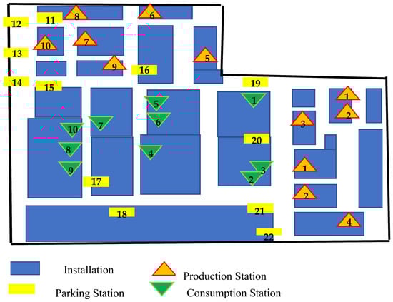
Figure 3.
AGV production system layout.
Table 4.
AGV circuits with the consumption rate and trolley capacity.
Table 5.
Distances between stations.
In the first stage, AGV circuit combinations with parking stations were calculated. I = 22 and S = 10, and at the end, 210 × 22 = 22,528 (GPij) values were calculated by the algorithm [50]. The next stage was about the selection of the optimum AGV fleet size with the GA. Genes reflect the parking station to which the AGV circuits are assigned. The population size was 300. Chromosomes are selected randomly such as 1-13-13-15-5-6-13-18-9-22. First, the AGV circuit was assigned to the first parking station. AGV circuits 2, 3, and 6 were used as an AGV pool in parking station 13. The fitness function is the sum of GPij, which indicates the required AGV number to fulfill production demands. GA solutions are given in Table 6. Table 6 and Table 7 are the solutions for the best chromosomes of the genetic algorithm, showing which AGV circuits will be assigned to which parking stations.
Table 6.
GA solutions.
Table 7.
GA solutions with a modified fitness function for circuits.
As a second objective, the AGV service time is included. With this approach, the minimum required AGVs that satisfy the minimum AGV investment and minimum service time lead to the minimum energy consumption, because AGVs use the minimum energy in waiting but moving on the ground increases the energy consumption. The pool combination that satisfies the minimum required AGVs with the minimum service time was computed as the optimal solution. The objective of the first fitness function was the required number of AGVs; then, the AGV service time was added as a second target to avoid unnecessary parking station assignments. To add this second objective, a new fitness function was defined by using coefficients separating the AGV number from the service time as follows,
Fitness function = 1000 × Required AGV number + Service time/1000
The GA solutions with the new fitness function are given in Table 7.
According to the results, some circuits were repeatedly assigned to the original parking stations; for example, AGV circuit 1 is usually assigned to the parking (production) station. The second observation was regarding the sharing of parking stations. When certain circuits do not share parking stations with other circuits, they use their own parking (production) station as the desired state. As a result, the suggested solution is 1-2-3-4-16-15-7-8-16-15. According to this solution, two pool systems should be created. The first pool should be at parking station 16, and AGV circuits 5 and 9 should use this pool. A second pool should be created at parking station 15, and AGV circuits 6 and 10 should use this pool. Other AGV circuits should use the production stations as parking stations. It was shown that the proposed approach provides a fleet size which requires five fewer AGVs, with a 29% reduction in the number of AGVs.
Additionally, the validity and efficiency of the results were checked with a simulation technique to determine the status of the production loss, if it exists. Figure 4 shows the simulation model designed to check the validation of the results obtained in this study. In the simulation model, there are ten AGV circuits and two AGV pools, and as a result, no production loss due to the AGV system was observed. The simulation model was run in Witness program to check the validity of the results [15].

Figure 4.
Simulation model.
It was obtained that AGV circuits 5 and 9 are assigned to parking station 16 and AGV circuits 6 and 10 are assigned to parking station 15. The model was run for 1100 min. As a result of the simulation, we conclude that the determined AGV number can provide the required transfers because the occupancy rate of consumptions stations is 100.
5. Determination of the Effect of System Parameters on the Required AGV Number
Until this part of the study, we have assumed that the parameters of the AGV system are considered at previously defined values and the results for the required AGV numbers were obtained with MILP and the GA. However, sometimes production demands may change; therefore, the AGV system must adjust to changing production demands. This stage is concerned with examining the number of AGVs in the case of a change in system parameters if the production requirements change. Although all system parameters of the AGV are taken within certain levels, as given in Table 8, there may be changes in speed, capacity, and distance due to change in production demands. In such a case, all calculations have to be redone. In order to avoid this situation, it is important to estimate the amount of AGVs for the new situation at a reduced computational cost and time lost. Especially in cases outside the defined system parameter levels, the results can be found by using intelligent-system-based estimation techniques, without using time-consuming MILP–GA or simulation-based analysis methods. Therefore, in this study, an ANN is proposed to predict the effects of the system parameters on the AGV number and to check the possibility of reducing the AGV number under changing conditions in production, such as what the effect will be if the speed is increased by 10%, how much AGVs are gained if the capacity is increased by 5%, or to check the possibility of decreasing the required number of AGVs due to changes in system parameters.
Table 8.
System input and output parameters.
An artificial neural network (ANN), the response surface method (RSM), and multiple linear regression (MLR) were used to examine the effect of the change in system parameters on the required AGV number. Multiple linear regression is a statistical modeling technique used to analyze data to make predictions of the response variable (y) with multiple explanatory variables (x1, x2, … xp) with linear relation. In other words, it is used to predict the outcome of the response variable [51]. The response surface method (RSM) explores the relationship between various explanatory variables and the response. The aim is to optimize this response [52]. Parameter optimization with RSM for one AGV circuit was analyzed in 2019 by Şenaras, A.E. [32].
A neural network is a mathematical model of how the brain works neurologically. It mathematically models the nerve cells to imitate the brain’s process of learning. It is structured with interconnected items called neurons included in layers. Artificial neurons are linked via artificial synapses and acquire knowledge through learning. The feed-forward neural network is an artificial neural network architecture, which is also called a multi-layer neural network. A feed-forward network is one in which information or signals are only sent in one direction, from input to output [53,54,55].
In this study, the neural network model was used as a surrogate model to predict the required number of AGVs by changing four parameters. A surrogate model is a statistical model which solves complex problems at a reduced computational cost by accurately approximating a function instead of solving the problem with expensive computational simulations. It is widely used in solving complex engineering optimization problems. Surrogate models are used when the outcomes of the problem cannot be easily computed, especially for complex optimization problems. They provide an efficient way to define models, which can be solved at a reduced computational cost instead of by complex simulations.
The structure of the ANN used in this study is shown in Figure 5. The ANN is composed of a three-layer network. The inputs were the velocity, charging time, distance, and hauled part count and the output was the number of required AGVs. Pearson correlation coefficient (R) and mean absolute percentage error (MAPE) values were examined to find the best ANN structure [53]. The hidden layer included five neurons. The training algorithms of Levenberg–Marquardt and Bayesian regularization were used to train the neural network model.
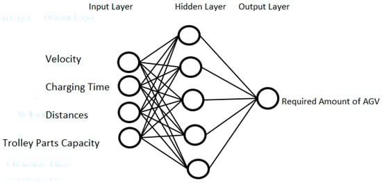
Figure 5.
The structure of the ANN model.
Cross-validation is a statistical technique to evaluate networks by partitioning the data into subsets of specified ratios. In this research, a hold-out method for cross-validation was used by partitioning the data into subsets, which are the data used for testing and validation and the data used for neural network model training. This technique is preferred as the dataset is small. The ANN model and predictions were saved when the Pearson correlation coefficient (R) of the test was higher than 0.998, as well as when finding better mean square error (MSE) values. The reason for choosing the MSE over the R-value is to prevent over-fitting and increase accuracy. For the dataset, 80% of the data are used as training, 10% for testing, and 10% for validation. The neural network model was run in Matlab [46]. The best performance for the training was realized with Bayesian regularization, and the performance was evaluated in terms of mean squared error (MSE) and Pearson correlation coefficient (R) values. The R-values for the neural network model were recorded for training and testing. All the R-values were computed as shown in Figure 6. Bayesian regularization backpropagation (BRB) and the Levenberg–Marquardt (LM) algorithm were used to train the neural network model. Bayesian regularization allows for better values for R (0.998) and the MSE (2.088 × 10⁻⁵). The R-value must be close as possible to 1. The ANN estimates successfully compared to RSM and MLR in R2 and mean absolute percentage error (MAPE), which were used to evaluate the prediction accuracy. They are performance evaluation results between the predicted and true value.
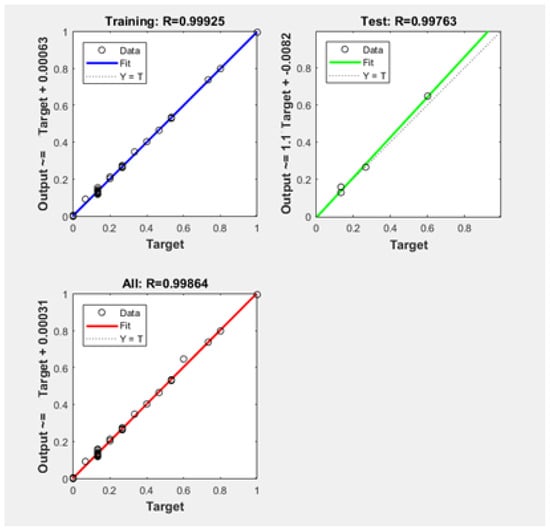
Figure 6.
ANN accuracy rates with R-values.
The effect of system parameters on the required AGV number was investigated for the velocity, charging time, distance, and trolley part capacity. These parameters and their minimum, maximum, and average values are given in Table 8.
A design of experiment (DOE) was carried out for the four determined system variables. Box–Behnken designs are experimental designs for response surface methodology. They do not contain an embedded factorial or fractional factorial design. Box–Behnken designs are created by combining factorial design with incomplete block designs, resulting in efficient solutions in terms of the number of runs required. This method allows us to produce effective solutions with a smaller number of trials than incomplete block design [52]. The Box–Behnken method was used, and 40 trials were carried out, including four factors and one repetition. The dataset is given in Table 9. The required AGV number was obtained by running the GA. RSM, ANN, and MLR were employed to examine the AGV number and the results were compared with the GA as shown in Table 9.
Table 9.
Required AGV numbers with ANN, RSM, and MLR.
RSM was run in Minitab [50]. The model successfully explains the effects of parameters on the system. The R2 value is 0.9911 and the corrected R2 value is 0.9807. P values were also obtained of less than 0.05. According to the model, the required number of AGVs can be expressed as follows:
Another investigation was realized with MLR using Matlab and the above equation was obtained as below (system parameters, Y, A, B, C, D are in a normalized form) [46],
Y = −0.1454 A + 0.336 B + 0.522 C − 0.2958 D
The ANN obtained the solution at a good rate with a reduced computational cost, time, and correction errors compared to the GA at 0.4% (ANN), 7% (RSM), and 24% (MLR) and within a 2 min computational time compared to 20 min for the simulation-based analysis. It can be concluded that there is no need to repeat the GA optimization approach or simulation process to achieve the minimum AGV fleet size, especially in case of production demand changes. The ANN is suitable, especially for cases with production demand changes, since the ANN learns from previous solutions and a new model design is not required to obtain the solution for new cases. In the present case, the ANN obtained the solution at a reduced computational cost compared to the GA and the simulation-based analysis.
6. Discussions and Conclusions
AGV projects involve significant investment costs. Firms tend to use low-cost AGVs to decrease the cost, but the scheduling and efficiency of the system may be low in the case of a lack of a central management system. Therefore, in this study, to overcome this situation, AGV pools were designed to decrease the required AGV number and to obtain the minimum required AGVs by increasing the utilization of AGVs through AGV pools to meet the demand in manufacturing.
The main objective of this research was to determine the optimum number of AGVs for decentralized AGV systems using the genetic algorithm (GA) and to estimate the required number of AGVs in the case of system parameter changes using an artificial neural network (ANN) and AGV pools with a reduced computational cost and time.
The main problems faced in the scheduling of a PLC or card-based and lane-guided decentralized systems are mostly due to excessive experimental times, limited data, and the complexity, since the variables increase exponentially with the number of AGV circuits, reducing the utility of the model in complex applications. Therefore, in this study, a GA and an ANN are proposed to determine AGV numbers in order to overcome the shortcomings caused by the exponential increase in the variables with the number of AGV circuits, the excessive experimental time, limited data, and the complexity.
In the first stage, a mixed integer model based on a time window analysis was developed to determine the optimum fleet size for low-cost AGVs with AGV pools. This approach successfully obtained optimum solutions for low numbers of AGV circuits, but a high computational time reduces the practicality of the model, especially in the case of complex systems. Therefore, a GA-based method was presented to handle this shortcoming, since Gas are an effective method in combinatorial optimization.
In this study, an ANN is proposed to predict the effects of the system parameters on the AGV number and to check the possibility of reducing the AGV number under changing production conditions. In the present case, the ANN obtained a solution at a good rate with reduced computational costs, time, and correction errors compared to the GA at 0.4% (ANN), 7% (RSM), and 24% (MLR), and within a 2 min computational time compared to 20 min for the simulation-based analysis. The results showed that the ANN provides solutions which can be used in workshops with a reduced computational cost and time. It can be concluded that there is no need to repeat the GA optimization approach or simulation process to achieve the minimum AGV fleet size, especially in case of production demand changes.
It was demonstrated that AGVs and pool combinations did not lead to any loss in production due to the lack of available AGVs. It was shown that the proposed approach provides a fleet size which requires five fewer AGVs, with a 29% reduction in the number of AGVs. The effects of system parameter changes were also investigated with artificial neural networks (ANNs) to estimate the required AGVs in the case of production requirement changes. The system designer could reduce the required AGV number by changing the system design and finding the most effective parameter using the proposed neural-network-based algorithm.
It was observed that the trolley capacity is the most effective parameter. The speed and distance are the second and third most influential factors on the required number of AGVs. In this study, the speed of AGVs was assumed as 20 m/min and an increasing velocity could have a negative effect on AGV system safety as well as AGV system reliability. This plays an essential role in evaluating the processes and defining the operating strategy according to different production requirement conditions.
Although several studies have been conducted on the design and control of AGV systems, they were mostly based on computer-assisted high-cost AGV systems. It was shown that this study contributes to this research area of PLCs or card-based and lane-guided decentralized AGV systems lacking a central management system through AGV pools using a GA and an ANN.
Although artificial neural network models, which are presented in this research, can be used efficiently for the present problem and similar types of problems, if the problem has a larger number of inputs, outputs, and system parameters and if the results of the neural network model are not acceptably accurate, then deep learning neural network architectures can be used to estimate the outputs in future research. The artificial learning model choice depends on the complexity of the problem due to the input and output parameters, the dataset, and other related modeling system parameters.
In this study, a GA is used as a heuristic optimization algorithm. An important feature of GAs as a heuristic optimization algorithm is their applicability to and efficiency in solving problems in a wide range of areas. Although in this research, a GA was applied as an efficient way to solve the present problem, i.e., to calculate the required AGV number assigned to every parking station, the efficiency and correctness of the results can be improved with hybrid GA-based heuristic optimization. Therefore, hybrid GA-based heuristic optimization techniques can be applied to the present study to compare the accuracy of solutions as a future research study.
Author Contributions
Conceptualization, O.M.Ş., F.Ö. and N.Ö.; Methodology, O.M.Ş., E.S., N.Ö. and F.Ö.; Software, O.M.Ş.; Writing—original draft, O.M.Ş.; Writing—review & editing, O.M.Ş. and F.Ö.; Supervision, E.S. and F.Ö.; Project administration, O.M.Ş. All authors have read and agreed to the published version of the manuscript.
Funding
This research received no external funding.
Institutional Review Board Statement
Not applicable.
Informed Consent Statement
Not applicable.
Data Availability Statement
Not applicable.
Conflicts of Interest
The authors declare no conflict of interest.
References
- Day, C.P. Robotics in industry—Their role in intelligent manufacturing. Engineering 2018, 4, 440–445. [Google Scholar] [CrossRef]
- Mozol, Š.; Krajčovič, M.; Dulina, Ľ.; Mozolová, L.; Oravec, M. Design of the System for the Analysis of Disinfection in Automated Guided Vehicle Utilisation. Appl. Sci. 2022, 12, 9644. [Google Scholar] [CrossRef]
- Ventura, J.A.; Rieksts, B.Q. Optimal location of dwell points in a single loop AGV system with time restrictions on vehicle availability. Eur. J. Oper. Res. 2009, 192, 93–104. [Google Scholar] [CrossRef]
- Bae, J.; Chung, W. A heuristic for path planning of multiple heterogeneous automated guided vehicles. Int. J. Precis. Eng. Manuf. 2018, 19, 1765–1771. [Google Scholar] [CrossRef]
- Aloui, K.; Guizani, A.; Hammadi, M.; Soriano, T.; Haddar, M. Integrated Design Methodology of Automated Guided Vehicles Based on Swarm Robotics. Appl. Sci. 2021, 11, 6187. [Google Scholar] [CrossRef]
- Bechtsis, D.; Tsolakis, N.; Vlachos, D.; Iakovou, E. Sustainable supply chain management in the digitalisation era: The impact of Automated Guided Vehicles. J. Clean. Prod. 2017, 142, 3970–3984. [Google Scholar] [CrossRef]
- Thakur, A. A Conceptual Market Analysis of Automated Vehicles for Logistics in Future. J. Supply Chain. Manag. Syst. 2022, 11, 25–38. [Google Scholar]
- Lee, C.; Ventura, J.A. Optimal dwell point location of automated guided vehicles to minimize mean response time in a loop layout. Int. J. Prod. Res. 2001, 39, 4013–4031. [Google Scholar] [CrossRef]
- Tubis, A.A.; Poturaj, H. Risk Related to AGV Systems—Open-Access Literature Review. Energies 2022, 15, 8910. [Google Scholar] [CrossRef]
- Van der Meer, J.R. Operational Control of Internal Transport (No. 1); ERIM Ph.D. Series Research in Management; Erasmus University Rotterdam: Rotterdam, The Netherlands, 2020; Available online: http://hdl.handle.net/1765/859 (accessed on 12 September 2021).
- De Ryck, M.; Pissoort, D.; Holvoet, T.; Demeester, E. Decentral task allocation for industrial AGV-systems with resource constraints. J. Manuf. Syst. 2021, 59, 310–319. [Google Scholar] [CrossRef]
- Schulze, L.; Behling, S.; Buhrs, S. AGVs in logistics systems, state of the art, applications and new developments. In Proceedings of the International Conference on Industrial Logistics (ICIL 2008): Logistics in a Flat World, Strategy, Management and Operations, Tel Aviv, Israel, 9–15 March 2008; pp. 256–264. [Google Scholar]
- Schulze, L.; Behling, S.; Buhrs, S. Automated guided vehicle systems: A driver for increased business performance. In Proceedings of the International Multiconference of Engineers and Computer Scientists, Hong Kong, China, 19–21 March 2008. [Google Scholar]
- Jia, L.; Shi, L.; Yao, J.; Dai, X.; Guo, G. Research on Intelligent Decision Method of Optimal Production Planning and AGV In-time Delivery in Mixed-Model Assembly Line. J. Phys. Conf. Ser. 2022, 2363, 012026. [Google Scholar] [CrossRef]
- Witness 22.b. Available online: https://www.lanner.com/en-us/technology/witness-simulation-software.html (accessed on 17 January 2022).
- Vis, I.F.A. Survey of research in the design and control of automated guided vehicle systems. Eur. J. Oper. Res. 2006, 170, 677709. [Google Scholar] [CrossRef]
- Soylu, M.; Özdemirel, N.E.; Kayaligil, S. A self-organizing neural network approach for the single AGV routing problem. Eur. J. Oper. Res. 2000, 121, 124–137. [Google Scholar] [CrossRef]
- İnanç, Ş.; Şenaras, A.E. AGV Routing via Ant Colony Optimization Using C. In Optimization Using Evolutionary Algorithms and Metaheuristics; CRC Press: Boca Raton, FL, USA, 2019; pp. 23–31. [Google Scholar]
- Bozorgi-Amiri, A.; Mahmoodian, V.; Fahimnia, E.; Saffari, H. A new memetic algorithm for solving split delivery vehicle routing problem. Manag. Sci. Lett. 2015, 5, 1017–1022. [Google Scholar] [CrossRef]
- Nishi, T.; Hiranaka, Y.; Inuiguchi, M.; Grossmann, I.E. A Decomposition Method with Cut Generation for Simultaneous Production Scheduling and Routing for multiple AGVs. In Proceedings of the 3rd Annual IEEE Conference on Automation Science and Engineering, Scottsdale, AZ, USA, 22–25 September 2007. [Google Scholar] [CrossRef]
- Rocak, S.N.; Bogdan, S.; Kovacic, Z.; Petrovic, T. Time windows based dynamic routing in multi-AGV systems. IEEE Trans. Autom. Sci. Eng. 2009, 7, 151–155. [Google Scholar] [CrossRef]
- Cardarelli, E.; Digani, V.; Sabattini, L.; Secchi, C.; Fantuzzi, C. Cooperative cloud robotics architecture for the coordination of multi-AGV systems in industrial warehouses. Mechatronics 2017, 45, 1–13. [Google Scholar] [CrossRef]
- Azimi, P. Alleviating the Collision States and Fleet Optimization by Introducing a New Generation of Automated Guided Vehicle Systems. Model. Simul. Eng. 2011, 2011, 210628. [Google Scholar] [CrossRef]
- Hsueh, C.F. A simulation study of a bi-directional load-exchangeable automated guided vehicle system. Comput. Ind. Eng. 2010, 58, 594–601. [Google Scholar] [CrossRef]
- Ventura, J.A.; Lee, C. Optimally locating multiple dwell points in a single loop guide path system. IIE Trans. 2003, 35, 727–737. [Google Scholar] [CrossRef]
- Ventura, J.A.; Pazhani, S.; Mendoza, A. Finding optimal dwell points for automated guided vehicles in general guide-path layouts. Int. J. Prod. Econ. 2015, 170, 850–861. [Google Scholar] [CrossRef]
- Nishi, T.; Hiranaka, Y.; Grossmann, I.E. A bilevel decomposition algorithm for simultaneous production scheduling and conflict-free routing for automated guided vehicles. Comput. Oper. Res. 2011, 38, 876–888. [Google Scholar] [CrossRef]
- Talbot, L. Design and Performance Analysis of Multistation Automated Guided Vehicle Systems. Ph.D. Dissertation, UCL-Université Catholique de Louvain, Ottignies-Louvain-la-Neuve, Belgium, 2003. [Google Scholar]
- Valmiki, P.; Reddy, A.S.; Panchakarla, G.; Kumar, K.; Purohit, R.; Suhane, A. A study on simulation methods for AGV fleet size estimation in a flexible manufacturing system. Mater. Today Proc. 2018, 5, 3994–3999. [Google Scholar] [CrossRef]
- Viharos, A.B.; Németh, I. Simulation and scheduling of AGV based robotic assembly systems. IFAC-Pap. 2018, 51, 1415–1420. [Google Scholar] [CrossRef]
- Tao, Y.; Chen, J.; Liu, M.; Liu, X.; Fu, Y. An estimate and simulation approach to determining the automated guided vehicle fleet size in FMS. In Proceedings of the 2010 3rd International Conference on Computer Science and Information Technology, Chengdu, China, 9–11 July 2010; Volume 9, pp. 432–435. [Google Scholar] [CrossRef]
- Şenaras, A.E. Parameter optimization using the surface response technique in automated guided vehicles. In Sustainable Engineering Products and Manufacturing Technologies; Academic Press: Cambridge, MA, USA, 2019; pp. 187–197. [Google Scholar]
- Chang, K.H.; Chang, A.L.; Kuo, C.Y. A simulation-based framework for multi-objective vehicle fleet sizing of automated material handling systems: An empirical study. J. Simul. 2014, 8, 271–280. [Google Scholar] [CrossRef]
- Rashidi, H.; Tsang, E.P. A complete and an incomplete algorithm for automated guided vehicle scheduling in container terminals. Comput. Math. Appl. 2011, 61, 630–641. [Google Scholar] [CrossRef]
- Saidi-Mehrabad, M.; Dehnavi-Arani, S.; Evazabadian, F.; Mahmoodian, V. An Ant Colony Algorithm (ACA) for solving the new integrated model of job shop scheduling and conflict-free routing of AGVs. Comput. Ind. Eng. 2015, 86, 2–13. [Google Scholar] [CrossRef]
- Nishi, T.; Morinaka, S.; Konishi, M. A distributed routing method for AGVs under motion delay disturbance. Robot. Comput.-Integr. Manuf. 2007, 23, 517–532. [Google Scholar] [CrossRef]
- Nishi, T.; Shimatani, K.; Inuiguchi, M. Decomposition of Petri nets and Lagrangian relaxation for solving routing problems for AGVs. Int. J. Prod. Res. 2009, 47, 3957–3977. [Google Scholar] [CrossRef]
- Moghaddam, B.F.; Ruiz, R.; Sadjadi, S.J. Vehicle routing problem with uncertain demands: An advanced particle swarm algorithm. Comput. Ind. Eng. 2012, 62, 306–317. [Google Scholar] [CrossRef]
- Moghadam, B.F.; Sadjadi, S.J.; Seyedhosseini, S.M. An empirical analysis on robust vehicle routing problem: A case study on drug industry. Int. J. Logist. Syst. Manag. 2010, 7, 507–518. [Google Scholar] [CrossRef]
- Fazlollahtabar, H. Parallel autonomous guided vehicle assembly line for a semi-continuous manufacturing system. Assem. Autom. 2016, 36, 262–273. [Google Scholar] [CrossRef]
- Lacomme, P.; Larabi, M.; Tchernev, N. Job-shop based framework for simultaneous scheduling of machines and automated guided vehicles. Int. J. Prod. Econ. 2013, 143, 24–34. [Google Scholar] [CrossRef]
- Rahman, H.F.; Janardhanan, M.N.; Nielsen, P. An integrated approach for line balancing and AGV scheduling towards smart assembly systems. Assem. Autom. 2020, 40, 219–234. [Google Scholar] [CrossRef]
- Han, W.; Xu, J.; Sun, Z.; Liu, B.; Zhang, K.; Zhang, Z.; Mei, X. Digital Twin-Based Automated Guided Vehicle Scheduling: A Solution for Its Charging Problems. Appl. Sci. 2022, 12, 3354. [Google Scholar] [CrossRef]
- Kim, B.I.; Park, J. Idle vehicle circulation policies in a semiconductor FAB. J. Intell. Manuf. 2009, 20, 709–717. [Google Scholar] [CrossRef]
- Miyamoto, T.; Inoue, K. Local and random searches for dispatch and conflict-free routing problem of capacitated AGV systems. Comput. Ind. Eng. 2016, 91, 1–9. [Google Scholar] [CrossRef]
- Matlab R17. Available online: https://www.mathworks.com/products/matlab.html (accessed on 12 December 2020).
- Tonelli, F.; Paolucci, M.; Anghinolfi, D.; Taticchi, P. Production planning of mixed-model assembly lines: A heuristic mixed integer programming based approach. Prod. Plan. Control 2013, 24, 110–127. [Google Scholar] [CrossRef]
- Ene, S.; Küçükoglu, İ.; Aksoy, A.; Oztürk, N. A genetic algorithm for minimizing energy consumption in warehouses. Energy 2016, 114, 973–980. [Google Scholar] [CrossRef]
- Ho, W.; Ho, G.T.; Ji, P.; Lau, H.C. A hybrid genetic algorithm for the multi-depot vehicle routing problem. Eng. Appl. Artif. Intell. 2008, 21, 548–557. [Google Scholar] [CrossRef]
- Minitab19. Available online: https://www.minitab.com/en-us/ (accessed on 16 November 2022).
- Tranmer, M.; Murphy, J.; Elliot, M.; Pampaka, M. Multiple Linear Regression, 2nd ed.; Cathie Marsh Institute Working Paper 2020-01. 2020. Available online: https://hummedia.manchester.ac.uk/institutes/cmist/archive-publications/working-papers/2020/2020-1-multiple-linear-regression.pdf (accessed on 22 March 2023).
- Montgomery, D.C. Design and Analysis of Experiments: Response Surface Method and Designs; John Wiley and Sons, Inc.: Hoboken, NJ, USA, 2005. [Google Scholar]
- Çallı, M.; Albak, E.I.; Öztürk, F. Prediction and Optimization of the Design and Process Parameters of a Hybrid DED Product Using Artificial Intelligence. Appl. Sci. 2022, 12, 5027. [Google Scholar] [CrossRef]
- Da Silva, I.N.; Spatti, D.H.; Flauzino, R.A.; Liboni, L.H.B.; dos Reis Alves, S.F. Artificial Neural Networks; Springer International Publishing: Cham, Switzerland, 2017. [Google Scholar] [CrossRef]
- Walczak, S.; Cerpa, N. Artificial Neural Networks. In Encyclopedia of Physical Science and Technology; Academic Press: Cambridge, MA, USA, 2003; pp. 631–645. [Google Scholar] [CrossRef]


Disclaimer/Publisher’s Note: The statements, opinions and data contained in all publications are solely those of the individual author(s) and contributor(s) and not of MDPI and/or the editor(s). MDPI and/or the editor(s) disclaim responsibility for any injury to people or property resulting from any ideas, methods, instructions or products referred to in the content. |
© 2023 by the authors. Licensee MDPI, Basel, Switzerland. This article is an open access article distributed under the terms and conditions of the Creative Commons Attribution (CC BY) license (https://creativecommons.org/licenses/by/4.0/).