Data-Based Modelling of Chemical Oxygen Demand for Industrial Wastewater Treatment

Abstract

The aim of wastewater treatment plants (WWTPs) is to clean wastewater before it is discharged into the environment. Real-time monitoring and control will become more essential as the regulations for effluent discharges are likely to become stricter in the future. Model-based soft sensors provide a promising solution for estimating important process variables such as chemical oxygen demand (COD) and help in predicting the performance of WWTPs. This paper explores the possibility of using interpretable model structures for monitoring the influent and predicting the effluent of paper mill WWTPs by systematically finding the best model parameters using an exhaustive algorithm. Experimentation was conducted with regression models such as multiple linear regression (MLR) and partial least squares regression (PLSR), as well as LASSO regression with a nonlinear scaling function to account for nonlinearities. Some autoregressive time series models were also built. The results showed decent modelling accuracy when tested with test data acquired from a wastewater treatment process. The most notable test results included the autoregressive model with exogenous inputs for influent COD (correlation 0.89, mean absolute percentage error 8.1%) and a PLSR model for effluent COD prediction (correlation 0.77, mean absolute percentage error 7.6%) with 20 h prediction horizon. The results show that these models are accurate enough for real-time monitoring and prediction in an industrial WWTP.

1. Introduction

The purpose of wastewater treatment is to remove suspended solids, organic matter, nutrients and harmful compounds from water so that its quality meets certain limit values before it is discharged back to the environment, typically into the sea or a river. It is very likely that the regulations and limit values for effluent quality set by the authorities will be more stringent in the future. The influent wastewater of an industrial wastewater treatment plant (WWTP) typically contains wastewater from several sources and, therefore, depending on the sourcing process and how it is operated, the quality (e.g., temperature, amount of nutrients and organic matter) and quantity of influent can vary significantly. These changes can be profound and occur quickly, but the heart of the wastewater treatment process, i.e., biomass, adapts slowly to changes. Drastic changes may be challenging for the operation of the treatment process and affect the quality of the effluent. In addition, the treatment process includes varying delays. Hence, there is a need for real-time monitoring of the WWTP process. Real-time monitoring may include online measurements but also soft sensors. In this study, the development of soft sensors for chemical oxygen demand is studied. These soft sensors can help reduce the pollution load and increase the efficiency of the WWTP process.

Chemical oxygen demand (COD) refers to the amount of oxygen consumed by the dissolved and suspended matter in a sample when exposed to a specific oxidising agent under specific conditions [1]. In simple terms, COD provides an estimate of the overall organic pollution or contamination level in water or wastewater. COD is a measure of the wastewater’s capacity to consume oxygen in chemical reactions. Typically in WWTPs, the COD is used to quantify the amount of harmful organic matter in the wastewater. The COD is, in many cases, measured in a laboratory offline from a sample or with an expensive online analyser. However, the harsh process conditions in WWTPs can cause deterioration and biofilm formation in analyser sensors that can cause interference, which can lead to reduced measurement precision over time [2]. Therefore, these sensors require constant maintenance, recalibration or replacement to keep them accurate, which is why soft sensors could prove to be a good alternative. A soft sensor can be utilised to indicate the malfunction of a hardware sensor or used instead of a hardware sensor for monitoring a process variable [3,4,5]. With a real-time estimator, process operators could match the process conditions to the incoming COD more accurately. Combined with a predictive effluent model, with the purpose of predicting the amount of COD discharged into the water basins, the WWTP operation could be optimised to treat the maximum amount of wastewater with minimal effort for both environmental and economic gain.

Regression models such as partial least squares regression (PLSR) and multiple linear regression (MLR) have been used to estimate the COD and other quality parameters in the past [6]. Mujunen et al. [7] utilised PLSR to estimate COD reduction among other parameters to analyse the treatment efficiency of a pulp and paper mill WWTP, using a large number of variables from the WWTP and a forward stepwise procedure to select the variables. One year later, in a similar study, Teppola et al. [8] utilised multiple linear regression, principal component regression and PLSR with a Kalman filter to update regression model coefficients to model COD reduction. Woo et al. [9] applied kernel partial least squares to model the COD, total nitrogen and cyanide of an industrial coke WWTP and compared the results with conventional linear PLSR. They found that the kernel partial least squares method was able to capture the nonlinearities of the WWTP and provide a better estimate for the modelled variables when compared to the linear PLSR. Dürrenmatt and Gujer [10] used generalised least squares regression (along with other modelling methods) to estimate the effluent COD in primary clarifiers and the ammonia concentration in activated sludge tanks. They found that simple linear models could be used accurately as soft sensors in a municipal wastewater treatment setting. Abouzari et al. [11] estimated the COD of a petrochemical wastewater treatment plant using various linear and nonlinear methods. They found that piece-wise regression linear regression provided relatively high accuracy and had better reliability compared to other methods. More recent studies on industrial applications have focused more on either nonlinear model structures or hybrid model structures and have been a popular research topic, as it is believed that these kinds of hybrid models could capture both nonlinear and linear behaviour [12].

Machine learning methods have also been a popular option in studies where soft sensing or prediction of process performance has been the focus [13,14,15,16]. Yang et al. [17] used a nonlinear autoregressive network with exogenous inputs (NARX) model to predict effluent COD and total nitrogen and compared the results with artificial neural network (ANN) models. Wang et al. [2] compared nine different machine learning algorithms in total to predict effluent COD. The resulting models demonstrated a high degree of precision. Zhang et al. [18] proposed a novel modelling method using dynamic Bayesian networks with variable importance in projection for soft sensor applications. The study included comparisons of their new modelling method to PLSR, ANN and other Bayesian networks. Many studies focus on nonlinear machine learning models, which provide little knowledge on how a modelled variable could be controlled [19]. These models are also difficult to implement in practice, which is why there is a significant need for models that could be directly derived from process measurements and easily implemented into practice.

In terms of studies where WWTP influent is monitored, municipal WWTPs have been a popular topic of research. This is largely due to rain having a large effect on the operation of municipal WWTPs, as the source of the incoming wastewater naturally greatly affects the characteristics of the wastewater and WWTP operation. Similar modelling methods have been used in studies where influent quality parameters are modelled [20,21,22,23]. However, since the main purpose of this research is to study industrial wastewater treatment, these studies are not further explored here.

This research aims to improve the utilisation of online process measurements in the context of industrial wastewater treatment plants. Online COD measurement is difficult and laborious to maintain. If left unmaintained, the measurement reliability is compromised. In addition, the sampling interval for online measurement is four hours, but with a soft sensor, the sampling interval can be reduced. Thus, this study focuses on models that can replace the online measurement device. The aims of this study are to form models for influent and effluent COD using available process data. The first target is to develop an accurate model for the influent, specifically to provide a basis for a soft sensor that estimates COD levels. This model gives online information about the influent COD. The second target is to construct a predictive model for effluent quality. The working principle of this model is similar to the influent model, but the goal is to predict the remaining COD in the wastewater before the wastewater is discharged, assuming the process conditions remain unchanged. The model proposed can be used for online monitoring of the WWTP. Because it predicts future effluent COD values, the information it provides can even be used to prevent undesired changes in the process. It is essential that models developed for both targets possess a high degree of interpretability and are sufficiently straightforward to enable direct implementation using process measurements. For this purpose, this work focuses on straightforward linear model structures.

WWTP process data contain many variables, from which one must be able to select the most important ones for the modelling. The selection of input variables is typically conducted based on available data using either an input variable selection method or process knowledge. The literature reports many techniques for automatic variable selection. This study does not use these, and thus these methods are not described here. An interested reader can find an excellent review of these, for example, by Guyon and Elisseeff [24]. In this study, an exhaustive algorithm is utilised to systematically test various combinations of online process variables from a pool of variables together with delays and model structures. Furthermore, suitable training windows are systematically browsed. By systematically sifting through the data, valuable information for modelling can be found. The key advantage of the whole approach is that it enables a comprehensive exploration of the entire dataset and model structures. In this study, the following model structures are examined: multiple linear regression (MLR), partial least squares regression (PLSR), autoregressive exogenous model (ARX), autoregressive moving average with exogenous input model (ARMAX) and least absolute shrinkage and selection operator (LASSO). Overall, this method offers a thorough approach to variable selection, enabling the extraction of important information from the available data and the creation of straightforward, interpretable models with real-world applicability.

This paper is organised in the following manner: Section 2.1 includes general knowledge about soft sensor development and the challenges related to it. Section 2.2 and Section 2.3 includes an introduction to the case WWTP and to the data collected from the plant. They outline the key characteristics and configuration of the WWTP, as well as how the data are used for modelling work. Section 2.4 discusses how these data were pre-processed to be used for modelling purposes. It explores the techniques used to transform the data to ensure their suitability for subsequent modelling purposes. Section 2.5 includes a discussion of the proposed modelling approach. Section 2.6 and Section 2.7 includes descriptions of the model structures utilised in this work, as well as the validation procedures used to assess their performance and accuracy. Lastly, Section 3 includes results from the modelling work and discussion.

2. Materials and Methods

2.1. Soft Sensor Development

Soft sensors are mathematical models that combine the outputs of one or more hardware sensors to estimate the targeted variable. A data-based soft sensor uses historical data to predict or estimate the variable of interest, even when direct measurements are not readily available. One of the main advantages of soft sensors is that they enable the estimation of hard-to-measure variables by a created mathematical model that consists of easy-to-measure variables. The mathematical models used in soft sensors are usually derived from data using statistical or machine learning methods. For the soft sensor output to be reliable, there needs to be a large amount of relevant data for soft sensor training [25].

One of the challenges is to find relevant data for model training. The data used for training and validation of the data-derived model should be of high quality to ensure a high-quality soft sensor. There can be various issues related to the data, such as nonlinear behaviour, different process phases and multicollinearity, which make modelling more difficult. Challenges related to information can relate to possible process deviations, sensor faults or over-fitting, or deterioration of the soft sensor model, all of which can make the development of soft sensor models more difficult. Lastly, challenges can be related to the implementation of expert knowledge. Leveraging process knowledge can be valuable in tasks such as pre-selecting relevant process variables or manually detecting outliers in the data, which can enhance the accuracy and reliability of the soft sensor model. Process knowledge can be utilised, for example, in the pre-selection of a process variable or manual detection of outliers [26]. Overall, these challenges in data acquisition, data-related issues, information challenges and utilisation of expert knowledge can pose significant hurdles in the development and successful implementation of high-quality soft sensor models.

2.2. Wastewater Treatment Plant

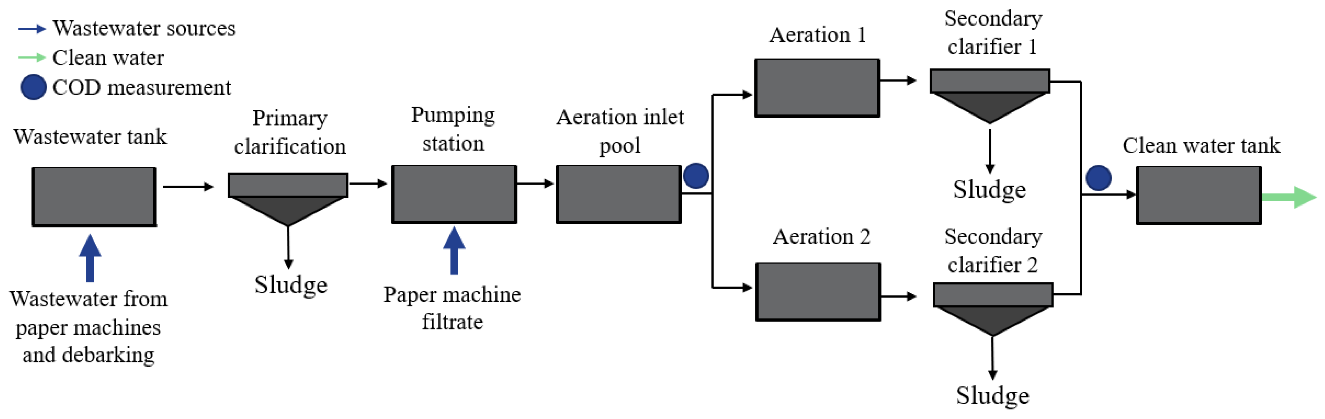
Data from a certain wastewater treatment plant related to a paper manufacturing plant were utilised in this study. A simplified schematic of the wastewater treatment plant in question is depicted in Figure 1. The wastewater leading to the WWTP originates from multiple sources. These sources include paper machines and the debarking process. The wastewaters from paper machines flow to the wastewater tank as individual streams. This tank also includes the wastewater from debarking. In addition, one wastewater stream (paper machine filtrate) enters the pumping station after primary clarification. The positions where online COD is measured are indicated in Figure 1.

The wastewater purification process at the plant consists of primary clarification as a primary treatment method and activated sludge process as a secondary treatment. The primary clarifier plays a crucial role in removing pollutants from the wastewater. It operates by allowing the settling of heavier or more readily separable solids at the bottom of the clarifier, forming a sludge layer, while the clarified water is collected from the top. The primary clarification helps improve the overall efficiency and cost-effectiveness of the process. After the primary clarifier, the paper machine filtrate stream is mixed with the rest of the wastewater. This combined wastewater is then pumped into a tank to wait for aeration. At this point, the wastewater quality measurements that are important for assessing the effectiveness of the treatment process and monitoring the performance of the plant are taken. Parameters such as COD, temperature, pH and other indicators provide valuable information about the overall condition of the wastewater going into aeration. The wastewater is then divided into two streams for the rest of the wastewater treatment. Next, the wastewater streams are sent to biological wastewater treatment, where the wastewater is mixed with air in a tank during the aeration process. The continuous circulation of air promotes the degradation of organic matter present in wastewater through the action of microorganisms. Following the biological treatment (aeration) stage, the wastewater undergoes the final treatment step in a secondary clarifier. In this step, the remaining pollutants and sludge are separated and removed from the wastewater, further improving its quality. The sludge is collected and further processed for disposal or potential reuse. Once the wastewater has undergone all the mentioned treatment steps, it is considered sufficiently treated and ready for discharge into the river. This final step ensures that the purified wastewater meets regulatory requirements and minimises its impact on the receiving water body.

2.3. Data Collection

Three datasets were received from an actual WWTP process, including online measurements from the automation system. Data from the related paper machine were also received. Online data were stored at a one-minute frequency.

Table 1. Dataset content information and its usage for modelling.

Data	Length	Variables	Variable Info	Dataset Usage
Dataset 1	1 year	44	Wastewater treatment process data	Effluent model development
Dataset 2	4.5 months	31	Wastewater treatment process data	Influent and effluent model development
Dataset 3	6 months	17	Wastewater data from paper machines	Influent and effluent model development

shows the relevant information about the datasets used.

Dataset 1 was the largest of the received datasets, containing one year’s worth of data. The initial dataset from the plant included 44 online measurements. From these measurements, 27 were chosen for the next step after the data pre-processing phase. Some variables were neglected because they contained no useful information. The measurements in Dataset 1 included data on temperature, pressure, flow rate, liquid level and various quality measurements from the wastewater process. Dataset 2 included similar data to Dataset 1, i.e., measurements from the wastewater treatment plant, but it covered only the summer period. Dataset 3 included measurements about WWTP influent obtained from the paper machine automation system and covered about the same time period as Dataset 2. These data were crucial for the development of the influent soft sensor. Dataset 2 spanned approximately 4.5 months, while Dataset 3 covered a period of six months. Datasets 2 and 3 were aligned and merged, and thus, about 1.5 month period from Dataset 3 was removed.

Dataset 1 was utilised as training data in developing the predictive effluent model. Dataset 2 served two purposes. Firstly, it was used as validation data for the predictive effluent model. Secondly, it was utilised in conjunction with Dataset 3 for developing an influent soft sensor model.

The device responsible for online COD measurement extracts periodic wastewater samples at a four-hour frequency. These samples undergo thorough analysis giving the online data that are promptly recorded within the automation system. This means that online data for the targeted variables are updated roughly every four hours. This applies to both the influent and effluent COD measurements.

2.4. Data Pre-Processing

The data were pre-processed using MATLAB^® software. The purpose of data pre-processing was to process the available data into the most complete form so that it could be used for modelling purposes. This included multiple steps. Firstly, variables that were constant (such as set point values for certain variables) were removed from the datasets. Variables were also removed if they included many Not a Number (NaN) values. Such variables contained no useful information from the modelling perspective.

The NaN values were replaced with interpolated values. Removal of NaN values from the data is important because they can cause issues with mathematical operations and modelling methods later. In this study, linear interpolation was employed to replace NaN values, utilising either the last known value or the next known value. The choice between these options depended on factors such as whether the variable began or ended with a NaN value.

Removal of NaN values was followed by an automatic outlier detection method. Outlier detection is an important step in data analysis and modelling. Firstly, it helps ensure data quality by identifying and addressing data errors, leading to higher data integrity and reliability. It also enables accurate statistical analysis by preventing distortions in data distribution and calculations of statistical measures. The ‘quartiles’ method was used to identify outlier points automatically [27]. In this method, data elements that are 1.5 interquartile range ($IQR$) below the lower quartile or above the upper quartile are automatically classified as outliers. The $IQR$ can be calculated as in Equation (1):

$$IQR=Q_3-Q_1,$$

(1)

where $Q_3$ represents the upper quartile (75 per cent of values from lowest to highest) and $Q_1$ the lower quartile (25 per cent of values from lowest to highest). After detecting the points that are above or below 1.5 $IQR$ of their respective quartile, the points were marked as outliers and changed to NaN values. This was performed so that the locations of these points would not go missing during deletion, as the removal of values from different parts between datasets would lead to discontinuity with the data timestamps if removed directly.

Usually, during this part of data pre-processing, data timestamps would also have to be fixed. However, the timestamps did not include any errors or multiple values, which is why the timestamps could be ignored during the data pre-processing and modelling as every data point was recorded at steady one-minute intervals.

Next, data points from the dataset, which were clearly outliers (such as negative pH values), were changed to NaN values. Other outlier points were detected by manually inspecting the data for possible outliers. Possible outlier points were left in the dataset if it was unclear whether the point was an outlier or a correct reading. The NaN values were then replaced with interpolated values similarly to before.

Once all outliers and NaN values were removed and interpolated from the data, the data were standardised. Standardisation is performed so that every variable uses the same common scale and can be performed with many different formulas. However, since most of the variables in the datasets were close to normally distributed, the standardisation was performed using the standard score formula (Equation (2)) [28]:

$$Z_i=\frac{x_i-\overline{x}}{S}$$

(2)

where $\overline{x}$ is the mean, and $S$ is the standard distribution of the variable being standardised. The standard score $Z_i$ represents how many standard deviations the actual value $x_i$ differs from the variable mean.

The datasets were then sampled utilising a moving median [29], where a median from a certain point window is used to represent all the data points from that window. The data points that were used to calculate the median were removed afterward, and only one point remained to represent all the removed values. Consequently, this means that the number of data points in each variable decreases drastically without losing any critical information. This type of averaging is beneficial as it allows more efficient calculation as well as filtering of the data. The efficient calculation is important later as an algorithm is utilised in the modelling part, which can be considered computationally heavy. The original minute data were reduced to a median of two-hour time intervals between data points.

As the last step of the pre-processing stage, the variables in the datasets were subjected to a nonlinear scaling algorithm with the purpose of making linear methodologies applicable to nonlinear cases. The nonlinear scaling algorithm was developed by Juuso [30]. The purpose of this method is to consider the nonlinear effects of the data. The scaling function transforms the data and scales it to a range of [−2, +2] using two monotonously increasing functions. One function is identified for the range of [−2, 0] and the other for the range of [0, +2]. Nonlinear scaling of variables is mainly utilised in regression modelling. Experiments were also performed without nonlinear scaling.

2.5. Modelling Methodology

Modelling of the influent COD and effluent COD was carried out by testing different model structures on both cases and tuning the optimal model parameters utilising an exhaustive algorithm. Figure 2 shows the overall flow of the modelling methodology steps, including the data pre-processing and analysis steps that were discussed in detail in the earlier section.

Since three different datasets were received, the first step was to divide the data into training, test and validation data for both cases. For the influent model, we combined Datasets 2 and 3 into one from the same time period. This was performed because Dataset 3 included data on incoming wastewater from the paper machines that were thought to be important for the estimation of influent COD. The aim was for every measurement that was used in modelling to originate from before or at the aeration inlet pool for the influent model. As discussed above, Dataset 3 fits this criterion perfectly. Variables that fit this criterion were picked from Dataset 2. Dataset 3 had to be trimmed a little due to being slightly longer than the other to make sure that the timestamps would fit correctly and be comparable to each other, as discussed in Section 2.3. It was noticed during the data pre-processing stage that Datasets 2 and 3 both had a section of data that was of poor quality that could not be used for modelling or validation. The majority of the data before the poor-quality section could be used for model training and testing and the later part for model validation.

For the effluent model, it was decided to use Dataset 1 for training and Dataset 2, which included nearly the same variables, for model validation. One deciding factor was that Dataset 1 was the longest of the three datasets and would contain the largest number of variables. However, some of the variables in Dataset 1 could not be utilised because they could not be found in Dataset 2. It was then decided which datasets would be used to model which case; the modelling work for each of the targets could be performed separately.

Both cases were modelled utilising a similar modelling strategy. The modelling work was performed by testing different model structures to see which model structure would fit the data best. Interpretable model structures were prioritised during the selection. The model structures and analysis methods tested included:

• Autoregressive exogenous model (ARX), autoregressive moving average with exogenous input model (ARMAX);
• Multiple linear regression (MLR), partial least squares regression (PLSR);
• Least absolute shrinkage and selection operator (LASSO).

After the model structure was chosen, it was tested on the chosen dataset by systematically testing for different attributes. In general, everything that could be tested systematically was considered. Features that could be tested varied depending on the chosen model structure. Systematic testing included:

• Time delays;
• Training windows;
• Variable combinations;
• Model orders (when needed).

Systematic testing of different attributes was conducted by utilising a design matrix in for-loop in MATLAB^® software. The design matrix is based on full factorial design is a statistically valid way to systematically test for different variables, in this case, different attributes [27]. The variables that were chosen for systematic testing were collected into a matrix pool. The numbers in the design matrix represent the indexes of the variables in the pool of variables. For example, with a model using five input variables, experiment 1 would consist of variables 1, 2, 3, 4 and 5; experiment 2 would consist of variables 1, 2, 3, 4 and 6. The design matrix for variables was constructed in the following manner:

• Choose the total number of variables for the pool of variables.
• Choose the number of variables for the model.
• Construct a full factorial design, where the total number of variables in the pool act as levels and the chosen number of variables as factors.
• Remove rows containing the same variable index.
• Remove rows that are not unique.

The number of chosen variables for the pool and the number of variables in the model essentially determine how many experiments there will be. However, before the formed design matrix can be used for modelling, some adjustments need to be performed. Rows that contain the same variable indexes (multiple same numbers) need to be removed from the matrix, as it is not beneficial to model cases where the same variable is taken into the model twice. The same applies to cases where the rows are not unique (same numbers, different order). The last two steps are not necessary but make the calculation time faster.

Time delays and model orders could be tested directly by creating a full factorial design of the desired range of time delays and model orders. For the influent models, time delays were tested between data points 1 and 16. With time intervals of two data points in the full factorial design, this meant that there were 32,768 possible time delay combinations to test for each attribute. A similar strategy was utilised when testing for different model orders. However, model orders were limited to the range from 1 to 6. For five variables, this would still mean 7776 different model order combinations. Lastly, different model training windows were tested over the dataset in a sliding window. The training window size also varied from a couple of hundred data points to the whole dataset. Therefore, the whole dataset was examined as thoroughly as possible to find the critical information.

The effluent model was modelled using the same strategy. However, it was found that fewer variables were needed to model the effluent COD, which is why more freedom was given to testing different attributes, as testing for three attributes is computationally significantly lighter compared to five variables. Furthermore, the effluent measurements are located farther away compared to the influent model, which is why it also made sense to increase the range for time delay testing.

In addition, tests with changes to the data pre-processing step were performed. These changes included modelling without the usage of nonlinear scaling. This could especially be performed with dynamic model structures when using more complex model orders. This is because one of the purposes of scaling the data with a nonlinear scaling function is that complex model structures are not needed in the modelling phase. Aside from tests with and without nonlinear scaling, modelling was performed with different values from the moving median window size. We experimented with different sampling rates for a 2, 4 and 8 h moving median value.

The purpose of the following pseudocodes is to provide further explanation of the modelling work. The purpose of these codes is to systematically test all possible variable and parameter combinations and store the results. This section includes pseudocodes for the ARX/ARMAX model structures and one for linear model structures. The pseudocode for the ARX model structure is presented in Figure 3.

As discussed in Section 2.5, multiple inputs are required for the code to work. Most importantly, the variable pool, design matrixes for the variables, model orders nb and delays. For the ARMAX model, an additional for loop is required for the model orders. The last loops are for determining the lengths and starting points of the varying sliding windows. It is important to consider the length of the data when defining the sliding windows and their starting points so that the whole data can be utilised with varying sliding windows and their starting points without producing an error. Inside the main for loop, the training data should be formed based on the indexes of the variable design matrix and the sliding window. An ARX model should be formed from this training data together with the selected delays and model orders. After the model was trained, validation data were formed based on the selected variables. The length of the validation data is the same every loop, as the model performance must be tested on data from the same period every time. Lastly, the results from the performance evaluation as well as important loop data, must be stored into a variable. This is important so that the results can be accessed afterward to see which variables, model orders, delays and training periods from the available data give the best results. The best model structure is then further tested with independent test data. The code for linear models worked in a similar manner (Figure 4). However, there are some differences. The linear model structures do not include model orders at all. The variables were also manually delayed. Finally, the code for linear models includes cross-validation in the loop.

2.6. Model Structures

Different model structures were utilised during this modelling work, including dynamic time series model structures such as the ARX and ARMAX. Aside from dynamic time series models, simple regression models such as PLSR and MLR were used. Lastly, we experimented with LASSO regression.

2.6.1. Dynamic Model Structures

Two dynamic model structures were chosen for this study. The ARX and ARMAX time series models are linear representations of a dynamic system [31]. The ARX model structure can be represented by the following Equation (3):

$$y\left(t\right)+a_{1}y\left(t-1\right)+\dots +a_{n_a}y\left(t-n_a\right)=b_{1}u\left(t-n_k\right)+\dots +b_{n_b}u\left(t-n_b-n_k+1\right)+e\left(t\right),$$

(3)

where $y\left(t\right)$ represents the model output at time $t$, and $n_a$ and $n_b$ represent the chosen model orders. The model delays are represented by $n_k$, which states how many input samples occur before that specific input affects the model output. Finally, $e\left(t\right)$ represents the white noise value of the system.

The ARMAX model structure is similar to that of the ARX. The major difference between the model structures is that the ARMAX model includes the moving average (MA) term [32]. The ARMAX model can be represented by the following Equation (4):

$$A\left(q\right)y\left(t\right)=B\left(q\right)u\left(t-n_k\right)+C\left(q\right)e\left(t\right),$$

(4)

where, similarly to the ARX model, $y\left(t\right)$ represents the model output at time $t$, $n_a$, $n_b$ and $n_c$ (included in A, B and C components) are the orders of the ARMAX model, $n_k$ represents the model delays and finally, $e\left(t\right)$ is the value of the white noise disturbance.

2.6.2. Static Model Structures

As stated above, of the static modelling methods, PLSR and MLR models were utilised in this study. The advantage of linear regression models is that they are interpretable. However, these model structures may fail to capture nonlinear or dynamic relationships. In this work, nonlinear scaling is utilised in the case of regression models, as stated in the section on nonlinear scaling, which means that nonlinearities are considered this way and should make these model structures perform well without losing their interpretability. Below (Equation (5)), the MLR model structure is given with n amount of input variables [33]:

$$\widehat{y}=b_0+b_1{x}_1+b_2{x}_2+\dots +b_n{x}_n,$$

(5)

where $\widehat{y}$ represents the predicted values; $x_n$ the predictor variables; $b_n$ represents the slope coefficients for the explanatory variables used in the model; and, finally, $b_0$ is the y-intercept term. The MATLAB^® function ‘regress’ was utilised to calculate the b coefficient estimates. For PLSR, the MATLAB^® function ‘plsregress’ was utilised [34]. The function follows the SIMPLS algorithm developed and discussed in detail by De Jong [35].

2.6.3. LASSO Regression

Lastly, we experimented with modelling methods that automatically choose variables for the models. LASSO regression does the variable selection and model training simultaneously [36]. It can be a suitable method, especially when there is a situation where data are abundantly available (especially a lot of variables). The LASSO method minimises the sum of squared error, while the model regression coefficients that are not important are given values close to zero [37]. The LASSO model solves the following Equation (6) for different values of $\lambda$:

$$\underset{{\beta }_0,\beta }{\min }\left(\frac{1}{2N}{\sum }_{i=1}^N{\left(y_i-{\beta }_0-x_i^T\beta \right)}^2+\lambda {\sum }_{j=1}^p\left|{\beta }_j\right|\right),$$

(6)

where $\lambda$ represents the regularisation term, $N$ represents the number of observations, $y_i$ represents the response at observation $i$, $x_i$ represents the input data at observation $i$, $p$ is the vector length, and ${\beta }_0$ and $\beta$ are the model parameters (regression coefficients).

2.7. Model Validation

The models were validated with a dataset that was not used during model training. In the case of ARX/ARMAX, a training window was utilised to systematically pick a part of the dataset, train a model and compare the results over the rest of the dataset. In the case of regression models, k-fold cross-validation was used to divide the datasets into training and test data. K-fold cross-validation divides the dataset into k number of folds (or partitions) that are nearly equal in size. After the data were divided, the k − 1 number of folds was used for model training, and the remaining data were used for model validation. This procedure was iterated k times, which means that each fold was successively utilised in validation, and the remaining data were used as training data [38]. The value for k was chosen to be 5 because there a large dataset was available and a separate independent validation dataset to test the effluent model on. With this k-value, it was believed that the results would be the most realistic as opposed to biased or optimistic. Monte Carlo repetitions were utilised to repeat this process 2000 times each time model training was performed. Both models were also subsequently tested with independent validation data afterward.

There are many ways to evaluate the performance of an identified model. Commonly utilised measurements include the root mean squared error (RMSE), mean absolute percentage error (MAPE) and the correlation coefficient (r). The following equations were used to calculate these performance metrics for the identified models to evaluate their performance [39]:

$$MSE=\frac{1}{N}{\sum }_{t=1}^N({\widehat{y}}_t-y_t),$$

(7)

$$RMSE=\sqrt{MSE},$$

(8)

$$AP{E}_t=\frac{\left|{\widehat{y}}_t-y_t\right|}{y_t}·100\%,$$

(9)

$$MAPE=\frac{1}{N}{\sum }_{t=1}^{N}AP{E}_t,$$

(10)

$$r_{xy}=\frac{{\sum }_{i=1}^n(x_i-\overline{x})(y_1-\overline{y})}{(n-1)S_x{S}_y},$$

(11)

where ${\widehat{y}}_t$ represents the predicted values, $y_t$ is the measured values, $N$ is the number of data points, $\widehat{y}$ is the response variables mean and $t$ represents time.

3. Results and Discussion

Modelling work was carried out as described in Section 2.5. In this section, the results are presented and discussed. A summary of the results for influent COD modelling are presented in

Table 2. Identified influent COD model structures and their performance metrics.

Inputs								Model Structure	Nonlinear Scaling	Training Data r	Training Data MAPE [%]	Training Data RMSE [mg/L]	Test Data r	Test Data MAPE [%]	Test Data RMSE [mg/L]
X 1	X 2	X 3	X 4	X 5	X 6	X 7	X 8
x	x	x	x	x				ARX	No	0.82	9.4	242.7	0.89	8.1	191.1
x	x	x	x	x				ARMAX	No	0.80	8.8	221.8	0.85	7.5	177.4
	x		x	x	x	x		MLR	Yes	0.46	15.03	399.8	0.4	17.1	371.4
	x		x	x		x	x	PLSR	Yes	0.72	10.87	245.9	0.74	7.8	147.6
x	x	x		x			x	LASSO	Yes	0.55	12.9	284.3	0.70	12.2	208.5

¹ Paper machine wastewater flow (1); ² paper machine wastewater flow (2); ³ paper machine wastewater flow (3); ⁴ aeration inlet pool pH; ⁵ pumping station wastewater temperature; ⁶ primary clarifier moment; ⁷ primary clarifier sludge amount; ⁸ temperature from neutralisation.

. After the best model parameters and structures were identified, a set of measurements were calculated to evaluate the performance of identified models, as discussed in Section 2.7.

The Dynamic model structures (ARX/ARMAX) performed the best when identifying the model for the influent COD. The ARX model demonstrated strong performance on both the training dataset, with a correlation coefficient of 0.82, MAPE of 9.4% and RMSE of 242.7 mg/L. Similarly, on the test dataset, the ARX model exhibited good results, achieving a correlation coefficient of 0.89, a MAPE of 8.1% and an RMSE of 191.1 mg/L. In terms of other models, PLSR and LASSO models also show reasonable performance with moderate r values and acceptable MAPE and RMSE values. The MLR model shows weaker performance compared with the other models (lower r values and higher MAPE and RMSE values). The most effective model (ARX) for the influent soft sensor model is depicted in Figure 5a. In this figure, the measured COD from the aeration inlet pool is represented by the black line, and the modelled COD is represented by the blue line as a function of time. The grey area that is plotted in the figures represents the 95% prediction interval estimated with training data. The ARX/ARMAX models had correlation coefficients of approximately 0.8. In both cases, the same variables were chosen for the model as input variables by the algorithm. The variables included two inflows from the paper machines, the flow from debarking, and pH and temperature from the aeration inlet pool. The addition of the moving average term to the model did not increase the correlation coefficients significantly. Hence, the ARX (orders: $n_a$: 6, $n_b$: (2 5 4 5 5)) model can be considered better as the model structure is simpler than the ARMAX model. The best model structures were attained when nonlinear scaling was omitted, and the dynamic model coefficients increased slightly. The identified model structure was then tested with validation data that had not been used in the model training. The results from this testing are presented in Figure 5b.

A summary of the results for effluent COD modelling are presented in

Table 3. Identified effluent COD model structures and their performance metrics.

Inputs								Model Structure	Nonlinear Scaling	Training Data r	Training Data MAPE [%]	Training Data RMSE [mg/L]	Test Data r	Test Data MAPE [%]	Test Data RMSE [mg/L]
X 1	X 2	X 3	X 4	X 5	X 6	X 7	X 8
x	x	x						PLSR	No	0.74	15.7	42.5	0.77	7.6	23.0
x		x	x					PLSR	Yes	0.71	12.5	28.6	0.68	14.5	36.3
x	x			x				MLR	Yes	0.68	12.4	29.9	0.67	25.1	59.4
x				x	x			LASSO	Yes	0.65	13.3	27.5	0.54	21.3	29.4
x						x	x	ARX	No	0.79	14.2	38.6	0.8	10.4	31.7
x						x	x	ARMAX	No	0.80	14.2	38.5	0.78	10.3	31.4

¹ Aeration inlet pool COD 2; ² aeration pH; ³ aeration oxygen 1; ⁴ aeration oxygen 2; ⁵ aeration air pressure; ⁶ paper machine wastewater flow (4); ⁷ pumping station flow rate; ⁸ debarking wastewater flow.

. For effluent predictive models, both the chosen dynamic model structures and the linear model, especially the PLSR structure without nonlinear scaling, worked well. The PLSR model without nonlinear scaling demonstrated good performance on both the training dataset, with a correlation coefficient of 0.74, MAPE of 15.7% and RMSE of 42.5 mg/L. On the test dataset, the PLSR model without nonlinear scaling also showed good results, with a correlation coefficient of 0.77, a MAPE of 7.6% and an RMSE of 23 mg/L. The PLSR model with nonlinear scaling also stands out as a well-performing model with high correlation coefficients (r values), low MAPE values and low RMSE values for both the training and test data. The MLR model with nonlinear scaling also performs reasonably well, although it has slightly lower correlation coefficients and higher MAPE and RMSE values compared with PLSR models. The identified ARX/ARMAX models worked best overall for the effluent prediction case based on correlation and MAPE values. However, because one of the goals of this research was model simplicity, more attention was also given to the linear regression model structures as they work for these data.

The identified PLSR model outputs (blue) and measured effluent COD (black) training data are plotted in Figure 6a. The variables chosen for this model were all located at the aeration inlet pool. The variables included the COD, pH and oxygen of the aeration inlet pool. The optimal delays for the identified PLSR model for these variables were 10, 10 and 20 data points, respectively. Since the minimum delay for the model is 10, this would indicate that effluent COD can be predicted 20 h in advance (one data point corresponds to two hours of data), assuming that there are no significant process changes. As discussed in Section 2.4, different moving median values were experimented with, and the 2 h period provided the best results from both the data analysis and modelling perspective. For the training data, the performance metrics show a correlation coefficient of 0.74. Similarly to the influent model, the identified model was tested on independent validation data. The results are presented in Figure 6b.

One explanation for why the correlation is much higher in the validation data when compared to the training data in the case of the effluent model is the number of data points. The training data contained approximately 4000 data points, whereas the validation dataset utilised was only 600 data points long, for the reasons discussed in Section 2.5. The COD measurement does not work as intended between data points 440 and 520 on the test data (Figure 6b), as the measurement output is constant for a long period of time. During this time, the model outputs significantly lower values and provides a much better estimate of the COD than a measurement device that is not working. Such malfunctions occur at constant intervals due to sensor fouling. Zoomed in perspective is presented in Figure 7.

Further model validation was performed by analysing the residuals of the created models. Histograms and normal probability plots were drawn for the training and test sets to evaluate model performance visually. A normal probability plot compares the residual to what would be expected if the data followed a normal distribution. The data are plotted in a way that should result in a straight line. If not, it suggests that the data do not conform to a normal distribution [27]. For the model to be considered good, the model residual should be close to normally distributed. The residuals for the influent COD soft sensor are plotted in Figure 8.

The histogram and the normal probability plot for the soft sensor training data residual in Figure 8a,b suggest that the residual appears to be normally distributed. Minor deviations can be observed at the tails of the distribution. The soft sensor test data residual in Figure 8c,d, on the other hand, shows more deviations at the tails yet shows a relatively straight line in the middle portion of the data. For the effluent COD predictive model, the training data in Figure 9a,b shows significant deviation for residual values that differ from the predicted values by one standard deviation (approx. 10% of values). A similar phenomenon could be observed in the effluent COD test data in Figure 9d, albeit to a lesser degree.

Lastly, some properties of the residual were calculated (

Table 4. Residual properties.

Residual	Range	Std. Deviation	Skewness	Kurtosis
Influent model training data	[−1.4, 2]	0.54	0.19	2.91
Influent model test data	[−0.8, 1.3]	0.43	0.74	3.3
Effluent model training data	[−2.4, 2.9]	0.67	0.63	4.3
Effluent model test data	[−1.2, 2.87]	0.55	0.34	3.84

) to numerically verify the observations. The range indicates the span of residual values, while the standard deviation represents the spread or variability around the model predictions. Skewness and kurtosis reveal the shape and potential outliers in the residual distribution. Monitoring these properties can help identify model deficiencies and guide further improvements.

The effluent training data exhibit residual values ranging from −1.4 to 2, with a standard deviation of 0.54. The distribution of residuals is moderately peaked (kurtosis = 2.91) and is slightly skewed (skewness = 0.19) with a longer tail on the right side. This suggests the presence of some outliers or heavy-tailed behaviour. These values are good for a model made with industrial data. The test data for the influent model show residual values ranging from −0.8 to 1.3. The standard deviation decreases slightly to 0.43, indicating a relatively smaller spread of residuals compared to the training data. The distribution remains slightly skewed (skewness = 0.74) and exhibits a higher peak (kurtosis = 3.3), suggesting a higher probability of outliers.

The effluent model’s training data exhibit residual values ranging from −2.4 to 2.9. The standard deviation of 0.67 indicates a larger spread of residuals compared to both the influent model’s training and test data. The distribution is similarly slightly skewed (skewness = 0.63) with a higher peak and heavier tails (kurtosis = 4.3), also suggesting the presence of extreme values or outliers. The test data for the effluent model show residual values ranging from −1.2 to 2.87. The standard deviation is 0.55, indicating a moderate spread of residuals. The distribution remains slightly skewed (skewness = 0.34) with a lower peak and lighter tails (kurtosis = 3.84) compared to the model’s training data. Overall, it seems that both models are a decent fit for their intended purposes, even if the models sometimes exhibit outliers. Considering that the models are a representation of a real wastewater treatment process, modelled with real data where situations and circumstances can vary significantly.

In general, the models perform well, especially when considering the complexity of the wastewater treatment process. Our study yielded results that are similar to previous industrial wastewater studies employing linear model structures. For example, Abouzari et al. [11] reported correlations between 0.68 and 0.835 for various linear models on test data. However, it should be noted that there can be significant differences between different industries on the formation of wastewater. When compared to studies that use machine learning methods for COD modelling, the linear model structures are unable to reach as high accuracies. For example, Güçlü and Dursun [13] were able to reach a correlation of 0.85 on the test data using an artificial network and a somewhat lower MAPE value (approximately 5%). However, as previously mentioned, linear model structures offer significant practical advantages such as interpretability, straightforward model adaptation and computational efficiency.

It is important to consider the specific requirements of the problem and the trade-off between model accuracy and complexity when choosing the most appropriate model, especially since the online hardware data are used mainly for monitoring purposes as laboratory analyses are required to ensure that effluent COD levels are within limits. Thus, the requirement for soft sensor accuracy is not that strict, and an acceptable margin of error ranges between 10 and 20%. This level of deviation is considered reasonable and tolerable, given the nature and objectives of the monitoring tasks at hand.

There are still some limitations and uncertainties in the models and, thus, possibilities for future work. One goal of this work was to develop interpretable models. However, the models developed here do not capture how the changes in manufactured paper grade affect the incoming COD to the WWTP well, for example. One solution could be to create multiple sub-models for each condition. However, this would require additional data fusion concerning the manufactured paper grades.

One of the limiting factors regarding the modelling work is that the data utilised for influent soft sensor modelling were acquired during a summer period. This may mean that the model can accurately estimate COD during similar summer conditions. Therefore, the knowledge of how the modelled solution would behave during winter conditions is still missing. The models have learned how the system behaved during the specific period that the data are from, which means that if the dynamics of the WWTP change over the years, the accuracy of these models may decrease. This is likely to happen when the WWTPs and the paper machine equipment are older, which may change the process dynamics. Therefore, it is important to keep in mind that the models developed here will occasionally require retraining or continuous adaptation for them to remain accurate.

It should also be noted that the dataset used for influent COD modelling only contained useful information regarding the flow rate of the incoming wastewater from the paper machines. With more useful quality data on the incoming wastewater streams, the soft sensor model could be significantly more accurate and simpler. Measurements from both the wastewater and the paper machines themselves could also potentially be utilised in modelling these kinds of model-based soft sensors.

Further research could include studies with more abundant data from process variables at the source of the wastewater. How the wastewater is formed naturally has a large effect on the overall quality of the wastewater, which is why data on the origin of the wastewater are valuable for influent soft sensor modelling. One interesting topic of research could include studies on how the influent soft sensor and the effluent predictive model could be combined.

The effluent predictive model relies on influent COD measurements as an input parameter. This value can be provided by the influent COD soft sensor model, and thus it is possible to predict the effluent COD without the need for physically measuring the influent COD. However, as discussed, for the models to replace the hardware sensor, model adaptation tools need to be developed. This would be a more challenging task if no online COD measurements were available. Instead, other measurements and laboratory data must be utilised to update the model coefficients effectively. This is not studied in this paper and would need more research.

The models developed need to be tested in practice. Implementation of these models is straightforward and only requires changes to the plant’s automation system to include the calculation of COD from the existing process measurements. This would give the plant a new monitoring tool, which can be useful as itself or in conjunction with the hardware sensor, especially in determining when the hardware sensor needs replacing and providing an estimate during that time, as depicted in Figure 7. The soft sensors also allow for lowering the sampling frequency of the hardware sensor, which in turn leads to reduced sensor maintenance costs as the measurement instrument is used less frequently. This can be very beneficial because the hardware sensor would be there to generate data for model adaptation but with lower costs.

4. Conclusions

The results indicate that measurements of paper machine wastewater streams can be utilised in estimating the total COD of wastewater incoming to the wastewater treatment plant with reasonable accuracy. The best model structure for the influent model was found to be an autoregressive-exogenous (ARX) model with low model orders. The chosen model structure was able to estimate incoming COD with a correlation coefficient of 0.82 and MAPE of 9.4% on the training data. For independent test data, the correlation and MAPE between the estimated model and measured outputs were 0.89 and 8.1%, respectively.

The results also indicate that measurements of the wastewater treatment plant are sufficient to predict the amount of COD present in the effluent. For the predictive effluent model, the partial least squares regression model was chosen from the results. Dynamic models such as the ARX models give similar results; however, more interpretable models were prioritised for this case as they were also able to obtain acceptable results. The chosen partial least squares regression model was able to estimate the effluent COD with a correlation of 0.74 and a MAPE of 15.7% for the training data. For the test data, the correlation and MAPE were 0.77 and 7.6%, respectively. The results seem reasonable considering the complexity of the wastewater treatment process. The delays indicate that the level of COD can be predicted approximately 20 h before the wastewater leaves the plant.