

A Novel Suspended-Sediment Sampling Method: Depth-Integrated Grab (DIG)

 , , ,
, , ,
Abstract
:1. Introduction
2. Materials and Methods
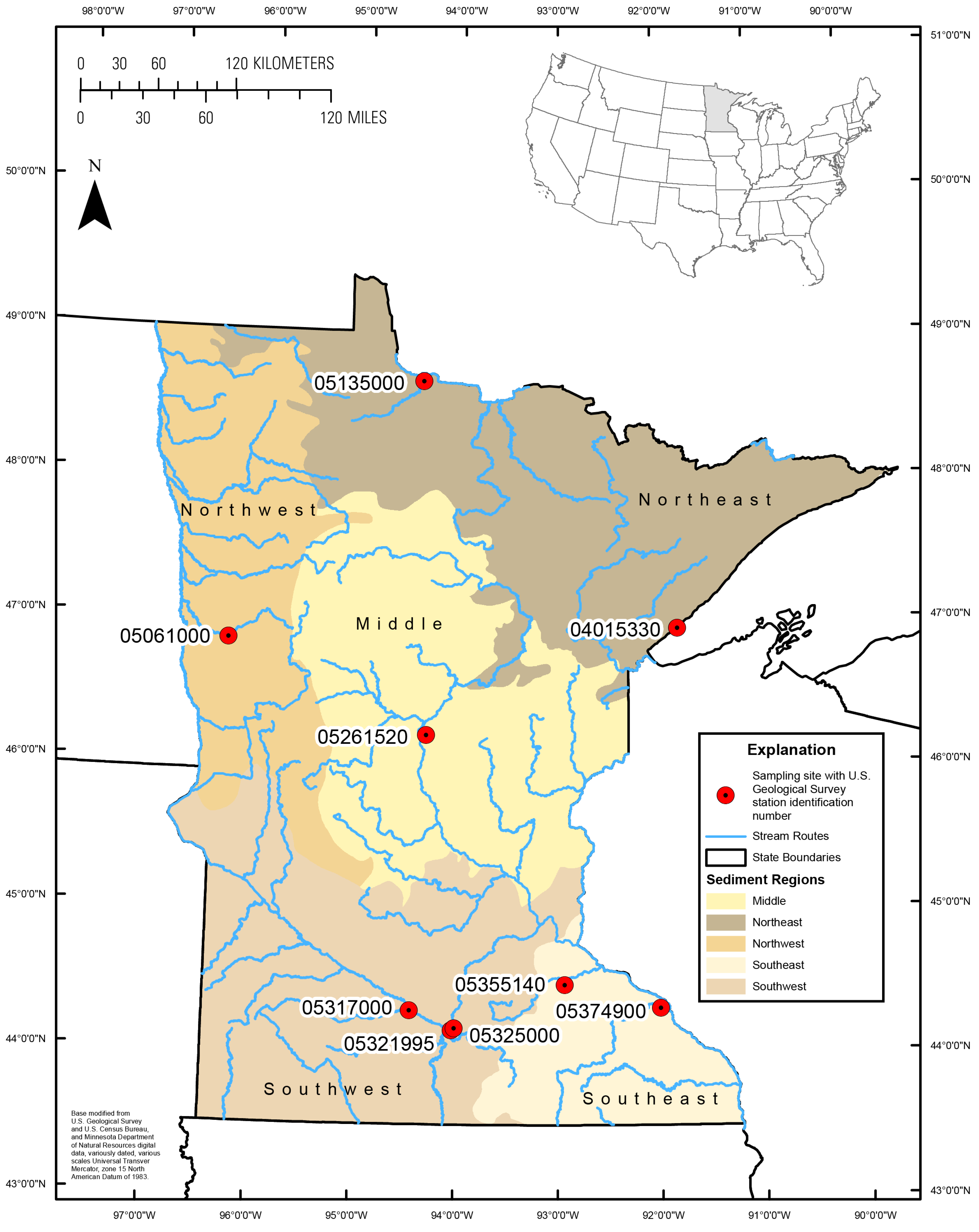
2.1. Study Area
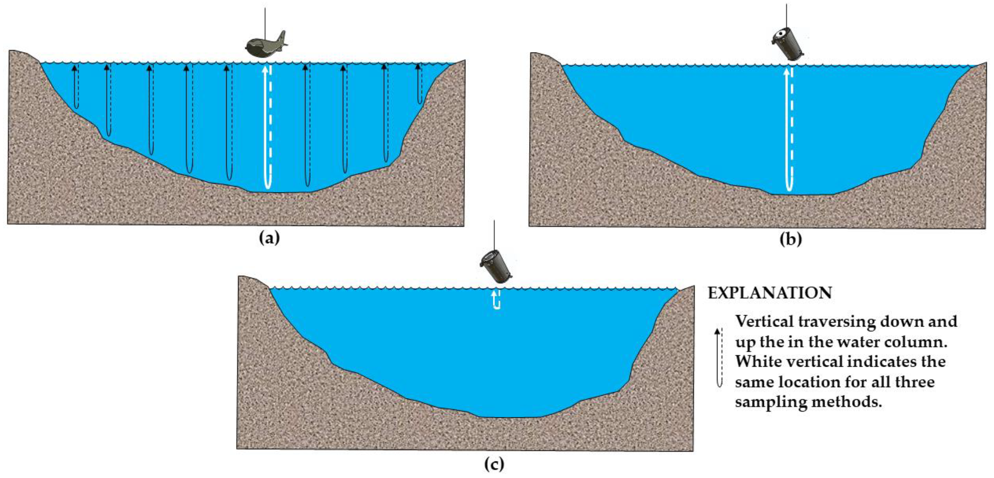
2.2. Equal-Width Increment or Equal-Discharge Increment (EWDI) Sampling Method
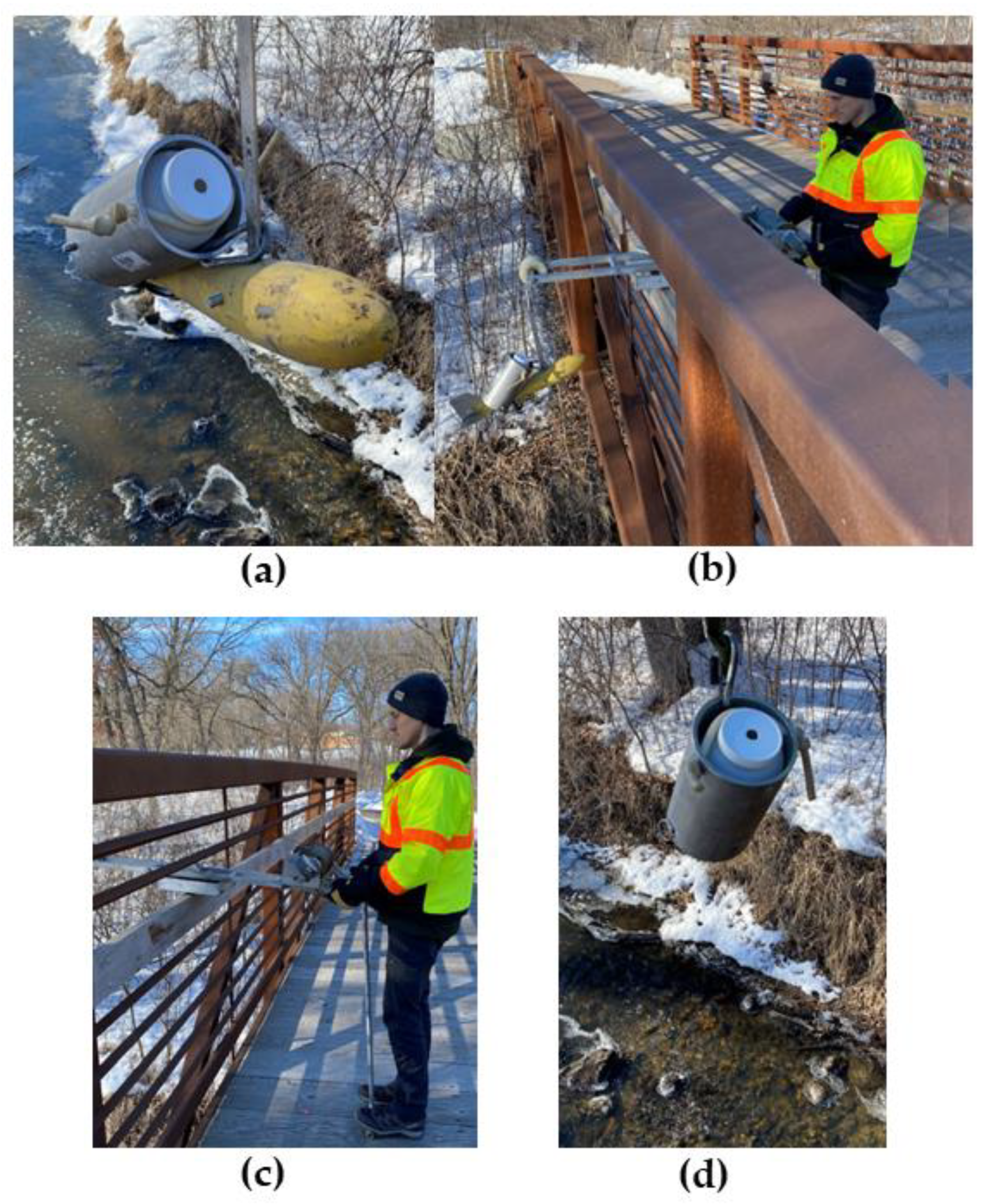
2.3. Depth-Integrated Grab (DIG) Sampling Method
2.4. Grab Sampling Method (Grab)
2.5. Suspended-Sediment Concentration Labratory Method (SSC, Fines, and Sands)
2.6. Total Suspended Solids Laboratory Method (TSS)
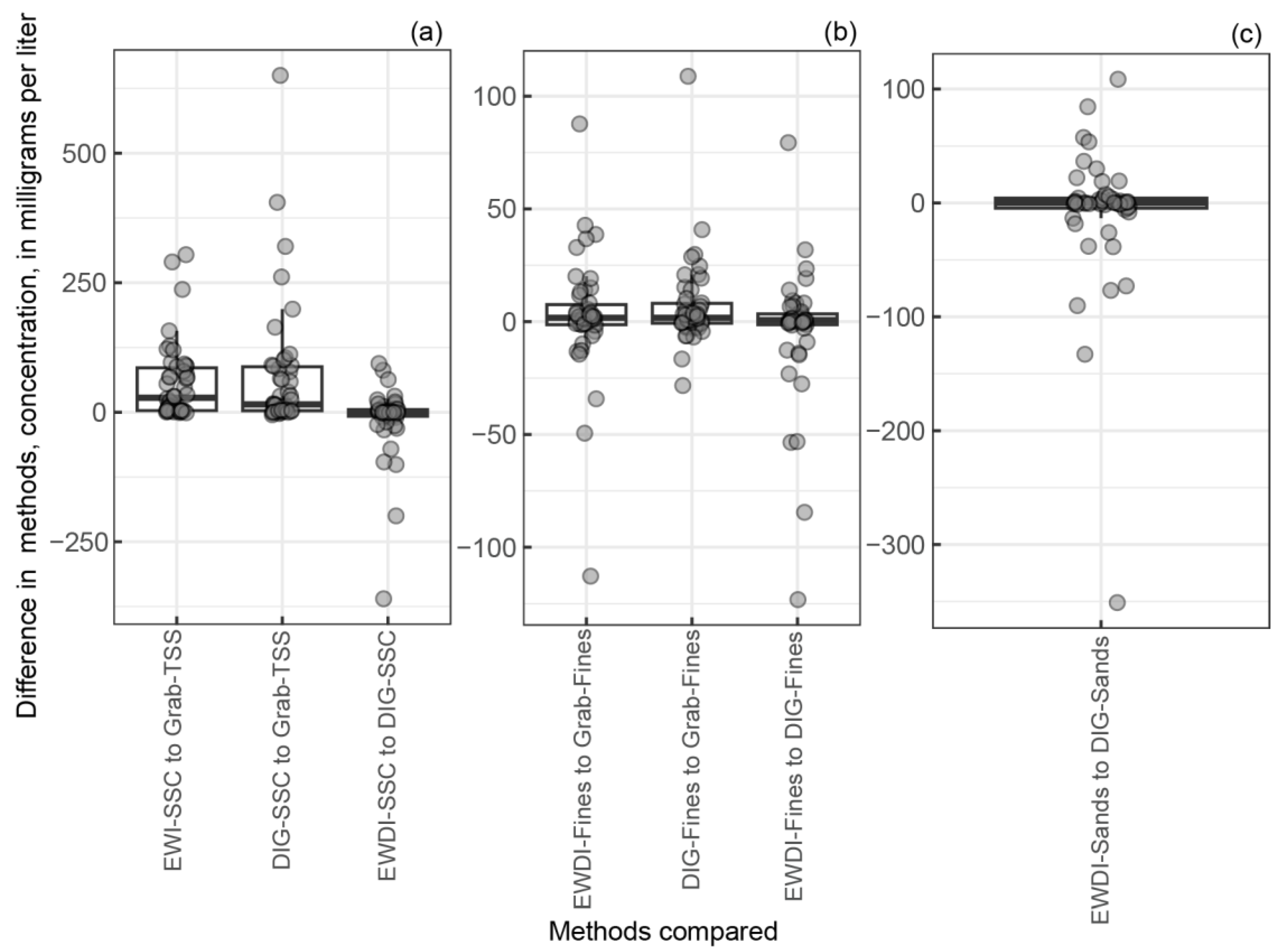
2.7. Data Analysis
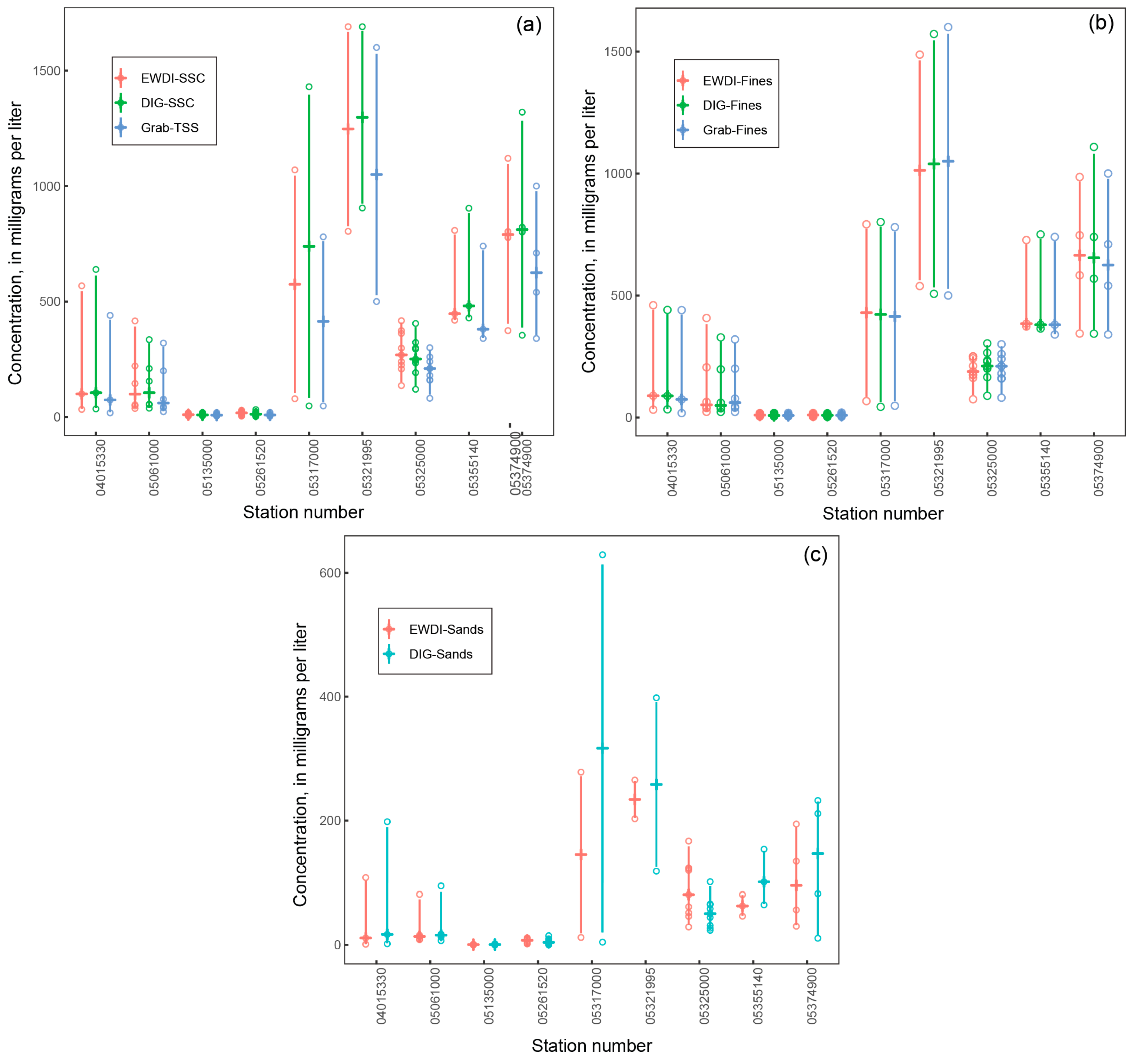
3. Results
4. Discussion
5. Conclusions
- (1).
- The DIG method does not replace isokinetic samplers and EWDI methods but shows promise as an alternative if users are unable to use isokinetic samplers and EWDI sampling methods.
- (2).
- The DIG method may only be used at sites that are well mixed horizontally. If a site is poorly mixed horizontally, EWDI methods with a DIG sampler can be used.
- (3).
- Grab sampling often occurs at lower velocities as isokinetic samplers are not recommended. The DIG-SSC method could replace grab sampling at lower velocities.
- (1).
- Grab-TSS may only be used as an estimate of suspended fines.
Supplementary Materials
Author Contributions
Funding
Informed Consent Statement
Data Availability Statement
Acknowledgments
Conflicts of Interest
Disclaimer
References
- Lewis, J.; Eads, R. Implementation Guide for Turbidity Threshold Sampling: Principles, Procedures, and Analysis; General Technical Report PSW-GTR-212; U.S. Department of Agriculture; Forest Service; Pacific Southwest Research Station: Albany, CA, USA, 2009; p. 87. [CrossRef] [Green Version]
- Steegen, A.; Govers, G. Correction factors for estimating suspended sediment export from loess catchments. Earth Surf. Process. Landf. 2001, 26, 441–449. [Google Scholar] [CrossRef]
- Guy, H.P. Fluvial Sediment Concepts. In U.S. Geological Survey Techniques of Water-Resources Investigations; Book 3, Chap. C1; U.S. Geological Survey: Reston, VA, USA, 1970; p. 55. Available online: https://pubs.usgs.gov/twri/twri3-c1/pdf/TWRI_3-C1.pdf (accessed on 6 February 2023).
- Clesceri, L.S.; Greenberg, A.E.; Eaton, A.D. Standard Methods for the Examination of Water and Wastewater, 20th ed.; American Public Health Association; American Water Works Association; Water Environment Federation: Washington, D.C., USA, 1998; variously paged. [Google Scholar]
- Gray, J.R.; Glysson, G.D.; Turcios, L.M.; Schwarz, G.E. Comparability of Suspended-Sediment Concentration and Total Suspended Solids Data; U.S. Geological Survey Water-Resources Investigations Report 00-4191; U.S. Geological Survey: Reston, VA, USA, 2000; p. 14. Available online: https://pubs.usgs.gov/wri/wri004191/ (accessed on 8 February 2023).
- Selbig, W.; Bannerman, R. Ratios of Total Suspended Solids to Suspended Sediment Concentrations by Particle Size. J. Environ. Eng. 2011, 137, 1075–1081. [Google Scholar] [CrossRef]
- Ellison, C.A.; Savage, B.E.; Johnson, G.D. Suspended-Sediment Concentrations, Loads, Total Suspended Solids, Turbidity, and Particle-Size Fractions for Selected Rivers in Minnesota, 2007 through 2011; U.S. Geological Survey Scientific Investigations Report 2013–5205; U.S. Geological Survey: Reston, VA, USA, 2014; p. 43. [CrossRef] [Green Version]
- Groten, J.T.; Johnson, G.D. Comparability of River Suspended-Sediment Sampling and Laboratory Analysis Methods; U.S. Geological Survey Scientific Investigations Report 2018-5023; U.S. Geological Survey: Reston, VA, USA, 2018; p. 23. [CrossRef]
- Groten, J.T.; Johnson, G.D. Comparability of different river suspended sediment sampling and laboratory analysis methods and the effect of sand. In Proceedings of the SEDHYD 2019 Conference on Sedimentation and Hydrologic Modeling, Reno Nevada, NV, USA, 24–28 June 2019; pp. 1–16. Available online: http://www.sedhyd.org/2019/proceedings/SEDHYD_Proceedings_2019_Volume3.pdf (accessed on 6 February 2023).
- Minnesota Legislature. Available online: https://www.revisor.mn.gov/rules/7050.0222/ (accessed on 15 March 2023).
- Ward, J.R.; Harr, C.A. Methods for Collection and Processing of Surface-Water and Bed-Material Samples for Physical and Chemical Analyses; U.S. Geological Survey Open-File Report 90-140; U.S. Geological Survey: Reston, VA, USA, 1990; p. 71. [CrossRef]
- Edwards, T.K.; Glysson, G.D. Field Methods for Measurement of Fluvial Sediment. In U.S. Geological Survey Techniques of Water-Resources Investigations; Book 3, Chap. C2; U.S. Geological Survey: Reston, VA, USA, 1999; p. 89. Available online: https://pubs.usgs.gov/twri/twri3-c2/pdf/TWRI_3-C2.pdf (accessed on 7 February 2023).
- Davis, B.E. A Guide to the Proper Selection and Use of Federally Approved Sediment and Water-Quality Samplers; U.S. Geological Survey Open File Report 2005-1087; U.S. Geological Survey: Reston, VA, USA, 2005; p. 20. [CrossRef]
- Guy, H.P. Laboratory Theory and Methods for Sediment Analysis. In U.S. Geological Survey Techniques of Water-Resources Investigations; Book 3, Chap. C1; U.S. Geological Survey: Reston, VA, USA, 1969; p. 58. Available online: https://pubs.usgs.gov/twri/twri3-c1/pdf/TWRI_3-C1.pdf (accessed on 9 February 2023).
- ASTM D3977–97; American Society for Testing and Materials (ASTM) International. Standard Test Methods for Determining Sediment Concentration in Water Samples. ASTM: West Conshohocken, PA, USA, 2000; Volume 11.02, Chap. Water (II). pp. 395–400.
- Performance Results Plus, US WBH-96 Weighted Bottle Sampler. Available online: https://prph2o.com/us-wbh-96-weighted-bottle-sampler/ (accessed on 15 March 2023).
- Performance Results Plus, D-74 Sediment Sampler. Available online: https://prph2o.com/d-74-sediment-sampler/ (accessed on 8 March 2023).
- Rasmussen, P.P.; Gray, J.R.; Glysson, G.D.; Ziegler, A.C. Guidelines and Procedures for Computing Time-Series Suspended-Sediment Concentrations and Loads from in-Stream Turbidity-Sensor and Streamflow Data. In U.S. Geological Survey Techniques and Methods; Book 3, Chap. C4; U.S. Geological Survey: Reston, VA, USA, 2009; p. 53. Available online: https://pubs.usgs.gov/tm/tm3c4/ (accessed on 8 February 2023).
- Wood, M.S.; Groten, J.T.; Straub, T.D.; Whealdon-Haught, D.R.; Griffiths, R.E.; Boldt, J.A.; Lucena, Z.N.; Brown, J.E.; Suttles, S.E.; Dickhudt, P.J. State of the Science and Decision Support for Measuring Suspended Sediment with Acoustic Instrumentation. In Proceedings of the SEDHYD 2023 Conference on Sedimentation and Hydrologic Modeling, St. Louis, MO, USA, 8–12 May 2023; pp. 1–16. Available online: https://www.sedhyd.org/2023Program/_program.html (accessed on 22 June 2023).
- Muneer, M.; Czuba, J.A.; Curran, C.A. In-Stream Laser Diffraction for Measuring Suspended Sediment Concentration and Particle Size Distribution in Rivers: Insights from Field Campaigns. J. Hydraul. Eng. 2023, 149, 05022007. [Google Scholar] [CrossRef]
- Minnesota Department of Natural Resources, Lands and Minerals. Available online: http://files.dnr.state.mn.us/lands_minerals/geologyhandbook.pdf (accessed on 3 March 2023).
- Lund, J.W.; Groten, J.T.; Karwan, D.L.; Babcock, C. Using machine learning to improve predictions and provide insight into fluvial sediment transport. Hydrol. Process. 2022, 36, e14648. [Google Scholar] [CrossRef]
- Gran, K.B.; Belmont, P.; Day, S.S.; Jennings, C.; Johnson, A.; Perg, L.; Wilcock, P.R. Geomorphic Evolution of the Le Sueur River, Minnesota, USA, and Implications for Current Sediment Loading; Geological Society of America Special Paper 451; Geological Society of America: Boulder, CO, USA, 2009; pp. 119–130. [Google Scholar] [CrossRef] [Green Version]
- Gran, K.B.; Belmont, P.; Day, S.S.; Jennings, C.; Lauer, J.W.; Viparelli, E.; Wilcock, P.R.; Parker, G. An Integrated Sediment Budget for the Le Sueur River Basin; Minnesota Pollution Control Agency (MPCA) Report wq-iw7-29o; Minnesota Pollution Control Agency: St. Paul, MN, USA, 2011.
- Ellison, C.A.; Groten, J.T.; Lorenz, D.L.; Koller, K.S. Application of Dimensionless Sediment Rating Curves to Predict Suspended-Sediment Concentrations, Bedload, and Annual Sediment Loads for Rivers in Minnesota; U.S. Geological Survey Scientific Investigations Report 2016–5146; U.S. Geological Survey: Reston, VA, USA, 2016; p. 68. [Google Scholar] [CrossRef] [Green Version]
- Ojakangas, R.W.; Matsch, C.L. Minnesota's Geology, 1st ed.; University of Minnesota Press: Minneapolis, MN, USA, 1982; p. 255. [Google Scholar]
- Sims, P.K.; Morey, G.G. Geology of Minnesota: A Centennial Volume; Minnesota Geological Survey: Minneapolis, MN, USA, 1972; p. 632. Available online: https://hdl.handle.net/11299/57318 (accessed on 6 February 2023).
- U.S. Geological Survey. USGS Water Data for the Nation; U.S. Geological Survey National Water Information System Database. 2023. Available online: https://waterdata.usgs.gov/nwis (accessed on 7 March 2023).
- National Water Quality Monitoring Council. Water Quality Portal. 2023. Available online: https://www.waterqualitydata.us/ (accessed on 15 March 2023).
- Wilcoxon, F. Individual Comparisons by Ranking Methods. Biom. Bull. 1945, 1, 80–83. [Google Scholar] [CrossRef]
- R Core Team. R: A Language and Environment for Statistical Computing. R Foundation for Statistical Computing. 2023. Available online: https://www.R-project.org/ (accessed on 8 February 2023).
- Federal Interagency Sedimentation Project. Best practices for FISP Bag Sampler Intake Efficiency Tests and Operational Velocities; 2013. Federal Interagency Sedimentation Project Memorandum 2013.01. Available online: https://water.usgs.gov/fisp/docs/FISP_Tech_Memo_2013.01.pdf (accessed on 12 June 2023).
- Manaster, A.E.; Landers, M.N.; Straub, T.D. Intake Efficiency Field Results for Federal Interagency Sedimentation Project Bag Samplers; U.S. Geological Survey Open-File Report 2022–1036; U.S. Geological Survey: Reston, VA, USA, 2022; p. 27. [CrossRef]


| Station Name | Station Number | Date from (yyyymmdd) | Date to (yyyymmdd) | Number of Samples |
|---|---|---|---|---|
| KNIFE RIVER NEAR TWO HARBORS, MN | 04015330 | 20180531 | 20190415 | 3 |
| BUFFALO RIVER NEAR HAWLEY, MN | 05061000 | 20190401 | 20190716 | 6 |
| NOKASIPPI RIVER NEAR FORT RIPLEY, MN | 05261520 | 20190402 | 20190923 | 8 |
| COTTONWOOD RIVER NEAR NEW ULM, MN | 05317000 | 20190418 | 20190904 | 2 |
| BLUE EARTH RIVER AT HWY 169 AT MANKATO, MN | 05321995 | 20180608 | 20180921 | 2 |
| MINNESOTA RIVER AT MANKATO, MN | 05325000 | 20180421 | 20190529 | 9 |
| LITTLE CANNON RIVER NEAR CANNON FALLS, MN | 05355140 | 20190323 | 20190702 | 3 |
| ZUMBRO RIVER AT KELLOGG, MN | 05374900 | 20180422 | 20180921 | 4 |
| EAST FORK RAPID RIVER NEAR CLEMENSTON, MN | 05135000 | 20190424 | 20190710 | 11 |
| EWDI-SSC (mg/L) | DIG-SSC (mg/L) | EWDI-Sands (mg/L) | DIG-Sands (mg/L) | EWDI-Fines (mg/L) | DIG-Fines (mg/L) | Grab-TSS (mg/L) | Water Depth (m) | Stream Width (m) | Q (cms) | |
|---|---|---|---|---|---|---|---|---|---|---|
| Min. | 4 | 3 | 0 | 0 | 2 | 2 | 3 | 1 | 12 | 3 |
| Max. | 1690 | 1690 | 278 | 629 | 1487 | 1572 | 1600 | 10 | 126 | 1823 |
| Mean | 267 | 279 | 52 | 60 | 215 | 219 | 221 | 3 | 49 | 277 |
| Med. | 90 | 80 | 13 | 15 | 65 | 52 | 76 | 2 | 37 | 16 |
| SD | 362 | 400 | 71 | 113 | 307 | 320 | 317 | 3 | 39 | 517 |
| First Method | Second Method | Median | p-Value |
|---|---|---|---|
| EWDI-SSC | DIG-SSC | 0 | 0.68 |
| EWDI-SSC | Grab-TSS | 28 | <0.01 |
| DIG-SSC | Grab-TSS | 15 | <0.01 |
| EWDI-Sands | DIG-Sands | 0.09 | 0.96 |
| EWDI-Sands | Grab-TSS | −33 | <0.01 |
| DIG-Sands | Grab-TSS | −47 | <0.01 |
| EWDI-Fines | DIG-Fines | 0.65 | 0.42 |
| EWDI-Fines | Grab-TSS | 1.72 | 0.06 |
| DIG-Fines | Grab-TSS | 1.67 | <0.01 |
Disclaimer/Publisher’s Note: The statements, opinions and data contained in all publications are solely those of the individual author(s) and contributor(s) and not of MDPI and/or the editor(s). MDPI and/or the editor(s) disclaim responsibility for any injury to people or property resulting from any ideas, methods, instructions or products referred to in the content. |
© 2023 by the authors. Licensee MDPI, Basel, Switzerland. This article is an open access article distributed under the terms and conditions of the Creative Commons Attribution (CC BY) license (https://creativecommons.org/licenses/by/4.0/).
Share and Cite
Groten, J.T.; Levin, S.B.; Coenen, E.N.; Lund, J.W.; Johnson, G.D. A Novel Suspended-Sediment Sampling Method: Depth-Integrated Grab (DIG). Appl. Sci. 2023, 13, 7844. https://doi.org/10.3390/app13137844
Groten JT, Levin SB, Coenen EN, Lund JW, Johnson GD. A Novel Suspended-Sediment Sampling Method: Depth-Integrated Grab (DIG). Applied Sciences. 2023; 13(13):7844. https://doi.org/10.3390/app13137844
Chicago/Turabian StyleGroten, Joel T., Sara B. Levin, Erin N. Coenen, J. William Lund, and Gregory D. Johnson. 2023. "A Novel Suspended-Sediment Sampling Method: Depth-Integrated Grab (DIG)" Applied Sciences 13, no. 13: 7844. https://doi.org/10.3390/app13137844
APA StyleGroten, J. T., Levin, S. B., Coenen, E. N., Lund, J. W., & Johnson, G. D. (2023). A Novel Suspended-Sediment Sampling Method: Depth-Integrated Grab (DIG). Applied Sciences, 13(13), 7844. https://doi.org/10.3390/app13137844