Two-Wire Power Line Microwave Communication Using Low-Loss Modes

Abstract

A closed-form solution for the common and differential modal currents induced on a pair of infinitely long parallel conductors by a source, field coupled to a power line, is derived. For lossy conductors, the current consists of a continuous spectrum of radiation modes and (for the common mode) a modified low-loss Sommerfeld–Goubau (SG) mode and (for the differential mode) a quasi-TEM mode. This model is used to investigate the influence of a parallel conductor on microwave power line communication systems. When the complete current spectrum is used, it is shown that the SG mode is not the primary reason why low-loss communication is possible on power lines for distances on the order of 100 m. Nevertheless, and consistent with previous research, microwave communication using power lines has advantages over free space communication, and for typical parameters, the performance of these systems can be enhanced if the power line contains more than one conductor.

1. Background

The propagation of a low-loss surface wave on an open waveguide consisting of a single lossy conductor in free space was investigated by Sommerfeld in 1899 and later, in 1907, extended to the case of dielectric-coated conductors by Harms [1,2,3]. In 1950, Goubau described the mode as a means of facilitating “wide-band long-distance communication” [4,5]. That work resulted in the identification of discrete propagation modes for lossy conductors, dielectric-coated conductors or other conductors with appropriately modified surfaces, as discussed by Collin [6] (pp. 718–720). Of interest, presented here is the Sommerfeld–Goubau (SG) mode on a bare lossy conductor.

In the early 1950s, a significant amount of work was reported by Goubau et al. and Dyott concerning the development of launchers for exciting this mode as well as investigations of environmental impacts, such as rain, snow and ice and the effects of bends on attenuation [4,5,7,8,9]. The launcher design work was heuristic and focused on matching the transverse variation of the source field to that of the SG mode. Coated wires were of special interest since the coating results in a more rapid decay of the field around the conductor, and experimental launchers for these modes were reported. At about the same time, Kikuchi studied the transition of quasi-TEM waves on a wire above earth to the SG mode as the frequency increased into the microwave region [10,11]. Little additional work on this mode was reported until 2004, when Wang and Mittleman suggested its use in the terahertz frequency range as a lower-loss waveguide than either metallic tubes or optical fibers. Specifically mentioned were spectroscopy, sensing and imaging applications but not communications [12]. In 2006, Wiltse discussed the possibility of low-loss transmission and the capability for transmitting high power in the millimeter-wave or terahertz frequency ranges [13]. The specific idea of using the SG mode for wide-bandwidth open-waveguide communication on power lines was introduced by Elmore in 2009 [14,15,16]. This was followed in 2016 by an announcement from AT&T concerning a project to use SG-mode propagation on power lines for broadband communication [17]. Interest in the area of broadband communication using this mode of propagation continues. For example, Galli, Liu and Guanxi, reported a model for estimating channel capacity for open waveguides constructed from lossy conductors [18].

In the past, a great deal of work has been conducted concerning the problem of exciting currents on infinite wires with and without loss when using voltage sources [19,20]. However, voltage sources are not appropriate for communication along energized electric power lines since a high-frequency source cannot be inserted into the line. Hence, field coupling is the only option. While research on designing SG-mode launchers was conducted in the 1950s, its emphasis was on dielectric-coated wires, given their more rapid transverse decay of fields.

A complete solution for induced current consists of both SG mode current and a current relating to the continuous spectrum of radiation modes. In 1964, a more rigorous theory for the excitation of the SG mode using a ring source of magnetic current (identical to a voltage source for the ring radius equal to the conductor radius) surrounding an infinite lossy conductor was reported by Cohn and King [21]. In addition to the SG mode current, they calculated the radiated fields using steepest descent integration (SDI). Unfortunately, calculating these radiated fields is not equivalent to calculating the current due to the continuous spectrum. This is because for field points near the conductor, the simple form of SDI in [21] is not accurate since the SG pole is close to the saddle point [6]. Because this field is needed to calculate the current via Ampere’s law, the current cannot be determined accurately. Hence, Ref. [21] did not provide a complete expression for the induced current (i.e., the SG mode and continuous spectrum).

In a recent publication, an investigation of propagation on an open wire as related to microwave communication systems on power lines was reported [22]. This paper was written in order to clarify the relationship between the discrete SG modal current and the total current since it is the total current that is relevant to the performance of these systems. More specifically, a closed-form solution for the current induced on an isolated infinitely long lossy conductor by a voltage source in series with it or an electric dipole in close proximity to it was found. This model included contributions from the continuous spectrum of radiation modes as well as the low-loss discrete SG mode. While the relative magnitudes of these two components were shown to be sensitive to frequency and wire conductivity, the total current on a lossy conductor is nearly the same as that for a perfect conductor over distances comparable to power line communication repeater spacing. Hence, it was shown to be possible to use a simple expression for the total current from antenna theory to evaluate the performance of these power line communication systems. Further, for observation points not near the source, the current induced by the voltage and dipole sources differs only by a known constant. Dipole sources were considered since voltage sources cannot be inserted into power line conductors. Finally, the advantage of a single-conductor communication channel over a wireless channel using high-gain antennas was quantified.

However, it was also noted in [22] that power line conductors are not isolated, and, given the fact that SG mode fields decay slowly in the transverse plane, the influence of parallel conductors could be important. Some recent work has appeared on the topic of the SG mode on a pair of wires, but it did not incorporate the full expression for current, which would include the continuous spectrum [23]. Hence, the impact of a parallel conductor is investigated in this paper. More specifically, a single additional conductor will be assumed parallel to the one that is discussed in [22]. The two-conductor case is considered since its solution can be decomposed into simple common and differential modes leading to additional insight into the solution.

2. Problem Definition and Exact Solution

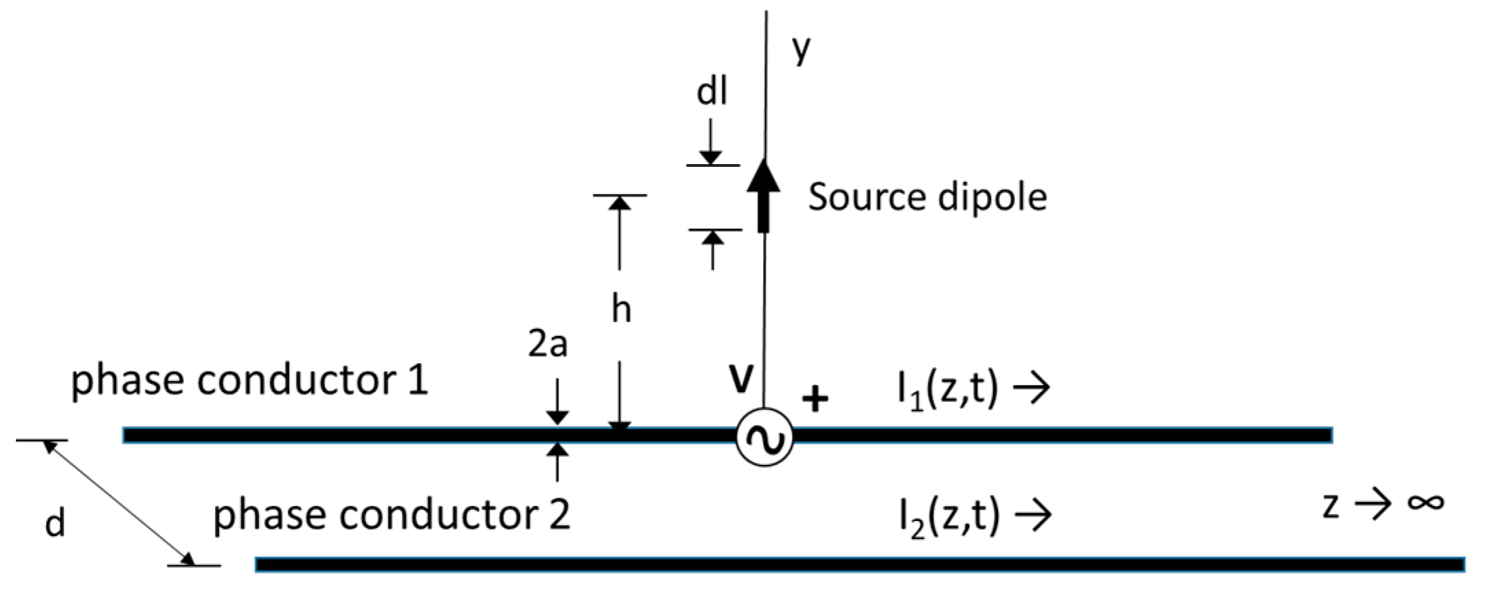
The problem is illustrated in Figure 1. Here, two infinitely long parallel lossy (conductivity ${\sigma }_w$) conductors, each of radius a and spaced a distance d apart are placed in the z direction. A voltage source of amplitude V volts at z = 0 and/or a y oriented elementary electric dipole of length dl at a distance h from the origin along the y-axis are used to excite currents on both conductors.

The approach here is to solve for the currents excited by the voltage source and then (later) to use the fixed relation between dipole and voltage sources derived in [22] to calculate those caused by the dipole source. The method is identical to that for the single-wire case except that there is an additional source of field (i.e., the second conductor). Hence, there will be two coupled equations (one for each conductor boundary condition) rather than a single one, as in [22].

A pair of homogeneous Fredholm integral equations of the second kind for the current ${\widehat{I}}_1\left(z\right)$ and ${\widehat{I}}_2\left(z\right)$ induced on this conductor (valid for $-\infty <z<\infty$) can be written as

$$\begin{array}{l}{\displaystyle \underset{-\infty }{\overset{\infty }{\int }}\left(g_{ez}^{11}\left(a,z-z^{\prime }\right){\widehat{I}}_1\left(z\prime \right)+g_{ez}^{12}\left(d-a,z-z^{\prime }\right){\widehat{I}}_2\left(z\prime \right)\right)d{z}^{\prime }+{\widehat{E}}_{ze}\left(-d/2+a,z\right)}\\ \hspace{1em}\hspace{1em}=-{\widehat{V}}_1\delta \left(z\right)+z_{iw}{\widehat{I}}_1\left(z^{\prime }\right)\\ {\displaystyle \underset{-\infty }{\overset{\infty }{\int }}\left(g_{ez}^{21}\left(d-a,z-z^{\prime }\right){\widehat{I}}_1\left(z^{\prime }\right)+g_{ez}^{22}\left(a,z-z^{\prime }\right){\widehat{I}}_2\left(z^{\prime }\right)\right)d{z}^{\prime }+{\widehat{E}}_{ze}\left(+d/2-a,z\right)}\\ \hspace{1em}\hspace{1em}=-{\widehat{V}}_2\delta \left(z\right)+z_{iw}{\widehat{I}}_2\left(z^{\prime }\right)\end{array}$$

(1)

$g_{ez}^{mn}\left(\rho ,z-z^{\prime }\right)$ is the axial electric field at $(\rho ,z)=(a,z)$ of a unit current of length $d{z}^{\prime }$ at $(0,z^{\prime })$, ${\widehat{E}}_{ze}\left(a,z\right)$ is the axial electric field at $(y,z)=(a,z)$ of the vertical electric dipole, and $\delta (z)$ is the Dirac delta function. $z_{iw}$ is the intrinsic impedance per unit length of the conductor, which for conductor sizes and higher frequencies of interest used here can be approximated as follows:

$$z_{iw}\cong {\left(\frac{\omega {\mu }_o}{2{\sigma }_w}\right)}^{1/2}\frac{\left(1+j\right)}{2\pi a},\hspace{1em}\left|k_{w}a\right|>>1$$

(2)

For (1), it has been assumed that the thin wire boundary condition ${\widehat{E}}_z\left(a,z\right)=z_{1w}\widehat{I}(z)$ is applied to the inside surface of each conductor radius. The time variation is $\exp (j\omega t)$, and the caret notation, ^, indicates a phasor quantity.

A formal solution to (1) for the current can be developed given that the integral equation is valid over the entire range of z from −∞ to ∞. The solution can be found by taking the spatial Fourier transform of both sides of (1). This transform and its inverse (i.e., $\tilde{F}\left(\gamma \right)$ and ${\tilde{F}}^{-1}\left(\gamma \right)$) used here are defined as follows:

$$\tilde{F}\left(f\left(z\right)\right)=\tilde{F}\left(\gamma \right)={\displaystyle \underset{-\infty }{\overset{\infty }{\int }}f\left(z\right)}{e}^{+j\gamma z}dz$$

(3)

$${\tilde{F}}^{-1}\left(\tilde{F}\left(\gamma \right)\right)=f\left(z\right)=\frac{1}{2\pi }{\displaystyle \underset{-\infty }{\overset{\infty }{\int }}\tilde{F}\left(\gamma \right)}{e}^{-j\gamma z}d\gamma$$

(4)

Here, the symbol ~ indicates a spatial Fourier transform with respect to the wire direction z that is dependent on the transform variable γ.

Taking the Fourier transform of (1) using (3) and the convolution identity

$$\tilde{F}\left[{\displaystyle \underset{-\infty }{\overset{\infty }{\int }}f\left(z^{\prime }\right)h\left(z-z^{\prime }\right)d{z}^{\prime }}\right]=\tilde{F}\left(f\left(z\right)\right)\tilde{H}\left(h\left(z\right)\right)$$

(5)

Results in the algebraic equations (Note: the physical dimensions of all terms are “volts” in the Fourier transform domain.)

$${\tilde{G}}_{ez}^{11}{\widehat{\tilde{I}}}_1\left(\gamma \right)+{\tilde{G}}_{ez}^{12}{\tilde{I}}_2\left(\gamma \right)+{\widehat{\tilde{E}}}_{ez}\left(-d/2+a,\gamma \right)=-{\widehat{V}}_1+z_{iw}{\widehat{\tilde{I}}}_1\left(\gamma \right)$$

(6)

$${\tilde{G}}_{ez}^{21}{\widehat{\tilde{I}}}_1\left(\gamma \right)+{\tilde{G}}_{ez}^{22}{\widehat{\tilde{I}}}_2\left(\gamma \right)+{\widehat{\tilde{E}}}_{ez}\left(d/2-a,\gamma \right)=-{\widehat{V}}_2+z_{iw}{\widehat{\tilde{I}}}_2\left(\gamma \right)$$

(7)

where ${\tilde{G}}_{ez}^{11}={\tilde{G}}_{ez}^{22}={\tilde{G}}_{ez}^{}\left(-d/2+a,\gamma \right)$ and ${\tilde{G}}_{ez}^{12}={\tilde{G}}_{ez}^{21}={\tilde{G}}_{ez}^{}\left(d/2-a,\gamma \right)$, while ${\widehat{\tilde{E}}}_{ez}\left(-d/2+a,h,\gamma \right)$ and ${\widehat{\tilde{E}}}_{ez}\left(d/2-a,h,\gamma \right)$ represent the axial electric field of the external source at each conductor, where h is the distance of the external source above the conductors. ${\widehat{V}}_1$ and ${\widehat{V}}_2$ represent the voltage at z = 0 of the source in series with each conductor.

The solution to these equations is formally valid at any frequency for which the conductor radius a is small compared to the other dimensions and the wavelength at the frequency of interest for which the conductor is appropriately modeled by its conductance ${\sigma }_w$.

Here, (The subscript notation 1/2 means 1 or 2. It should not be confused with the superscript ½ which means square root)

$${\tilde{G}}_{ez}\left(x-x_{1/2},\gamma \right)=\frac{1}{4\omega {\epsilon }_0}\left({\gamma }^2-k_0^2\right)H_0^{\left(2\right)}\left({\left(k_0^2-{\gamma }^2\right)}^{1/2}{\rho }_{1/2}\right)$$

(8)

where ${\rho }_{1/2}=\left|x-x_{1/2}\right|$ and $\mathrm{Im}{\left(k_0^2-{\gamma }^2\right)}^{1/2}\le 0$

Equations (6) and (7) can be written more compactly in matrix form as follows:

$$\left[\begin{array}{cc}{\tilde{G}}_{ez}^{11}-z_{iw}& {\tilde{G}}_{ez}^{12}\\ {\tilde{G}}_{ez}^{21}& {\tilde{G}}_{ez}^{22}-z_{iw}\end{array}\right]\left[\begin{array}{c}{\widehat{\tilde{I}}}_1\\ {\widehat{\tilde{I}}}_2\end{array}\right]=\left[\begin{array}{c}-{\widehat{V}}_1-E_{ez}^1\\ -{\widehat{V}}_2-E_{ez}^2\end{array}\right]$$

(9)

where (given symmetry and reciprocity) ${\tilde{G}}_{ez}^{11}-z_{iw}={\tilde{G}}_{ez}^{22}-z_{iw}$ and ${\tilde{G}}_{ez}^{12}={\tilde{G}}_{ez}^{21}$. ${\widehat{\tilde{E}}}_{ez}^1$ and ${\widehat{\tilde{E}}}_{ez}^2$ are, respectively, the axial electric fields of the external source evaluated at the bottom surfaces of conductors 1 and 2.

The square matrix in (9) is 2 × 2. It is known that if it has 2 distinct eigenvalues, then it has two distinct eigenvectors that are orthogonal with respect to it. It is also known that any two-element vector (e.g., $[\widehat{\tilde{I}}]$) can be expanded in this set of eigenvectors so that

$$\left[\widehat{\tilde{I}}\right]=\left[\eta \right]\left[{\widehat{\tilde{I}}}_{gm}\right]$$

(10)

where [${\widehat{\tilde{I}}}_{gm}$] is the matrix of the “geometric component” amplitudes (often referred to in the power engineering literature simply as “mode” amplitudes), and $\left|\eta \right|$ is the square matrix (by columns) of normalized eigenvectors of the square matrix in (9). Since the matrix in (9) is symmetric, it can be written as follows:

$$\left[\begin{array}{cc}A& B\\ B& A\end{array}\right]$$

(11)

The eigenvalues of this matrix (λ) (not to be confused with λ, which is used elsewhere to designate “wavelength”) are defined by

$$\left[\begin{array}{cc}A& B\\ B& A\end{array}\right]\left[\begin{array}{c}{q}_a\\ q_b\end{array}\right]=\lambda \left[\begin{array}{c}{q}_a\\ q_b\end{array}\right]$$

(12)

where the vectors $\overline{q}={\left[q_a,q_b\right]}^T$ are its eigenvectors. (not to be confused with q, which is used elsewhere to represent charge). Since (12) represents a homogeneous set of equations, it only has a solution if

$$\left|\hspace{1em}\begin{array}{cc}A-\lambda & B\\ B& A-\lambda \end{array}\hspace{1em}\right|=0$$

(13)

This occurs when the quadratic

$${\lambda }^2-2A\lambda +\left(A^2-B^2\right)=0$$

(14)

Hence, the eigenvalues are

$${\lambda }_{1/2}=A\pm B={\tilde{G}}_{ez}^{11}-z_{iw}\pm {\tilde{G}}_{ez}^{12}$$

(15)

The eigenvectors can be found by inserting the eigenvalues into (12) as

$$\left[\begin{array}{cc}\mp B& B\\ B& \mp B\end{array}\right]\left[\begin{array}{c}{q}_a\\ q_b\end{array}\right]=0$$

(16)

Given that the matrix in (16) is symmetric, its eigenvectors are simply

$${\overline{q}}_1=a_1\left[\begin{array}{c}1\\ 1\end{array}\right] \mathrm{and} {\overline{q}}_2=a_2\left[\begin{array}{c}1\\ -1\end{array}\right]$$

(17)

where a₁ and a₂ are arbitrary constants. ${\overline{q}}_1$ represents the common component (again often called the “common mode”), which has equal currents on each conductor, and ${\overline{q}}_2$ represents the differential component (again often called the “differential mode”).

These eigenvectors can be written as a matrix of eigenvectors (by columns) that are normalized to a magnitude of 1, as follows:

$$\left|\eta \right|=\frac{1}{\sqrt{2}}\left[\begin{array}{cc}1& 1\\ 1& -1\end{array}\right]$$

(18)

If the column matrix of conductor currents ${\widehat{\tilde{I}}}_1$ and ${\widehat{\tilde{I}}}_2$ is expanded in the eigenvectors of the symmetric matrix, then

$$\left[\begin{array}{c}\hspace{1em}{\widehat{\tilde{I}}}_1\hspace{1em}\\ {\widehat{\tilde{I}}}_2\end{array}\right]=\left[\eta \right]\left[\begin{array}{c}{\widehat{\tilde{I}}}_{gm1}\\ {\widehat{\tilde{I}}}_{gm2}\end{array}\right]$$

(19)

where ${\widehat{\tilde{I}}}_{gm1}$ and ${\widehat{\tilde{I}}}_{gm2}$ are the “geometric mode” amplitudes.

If (19) is substituted into (9), the entire equation is pre-multiplied by the inverse matrix ${\left[\eta \right]}^{-1}$, which (in this case) is equal to $\left[\eta \right]$.

$$\frac{1}{2}\left[\begin{array}{cc}1& 1\\ 1& -1\end{array}\right]\left[\begin{array}{cc}{\tilde{G}}_{ez}^{11}-z_{iw}& {\tilde{G}}_{ez}^{12}\\ {\tilde{G}}_{ez}^{21}& {\tilde{G}}_{ez}^{22}-z_{iw}\end{array}\right]\left[\begin{array}{cc}1& 1\\ 1& -1\end{array}\right]\left[\begin{array}{c}{\widehat{\tilde{I}}}_{gm1}\\ {\widehat{\tilde{I}}}_{gm2}\end{array}\right]=\frac{1}{\sqrt{2}}\left[\begin{array}{cc}1& 1\\ 1& -1\end{array}\right]\left[\begin{array}{c}-{\widehat{V}}_1-{\widehat{\tilde{E}}}_{ze}^1\\ -{\widehat{V}}_2-{\widehat{\tilde{E}}}_{ze}^2\end{array}\right]$$

(20)

However, pre-multiplying and post-multiplying a matrix by a matrix of its eigenvectors results in a diagonalized matrix of eigenvalues, as follows:

$${\left[\eta \right]}^{-1}\left[\begin{array}{cc}{\tilde{G}}_{ez}^{11}-z_{iw}& {\tilde{G}}_{ez}^{12}\\ {\tilde{G}}_{ez}^{21}& {\tilde{G}}_{ez}^{22}-z_{iw}\end{array}\right]\left[\eta \right]=\left[\begin{array}{cc}{\tilde{G}}_{ez}^{11}-z_{iw}+{\tilde{G}}_{ez}^{12}& 0\\ 0& {\tilde{G}}_{ez}^{22}-z_{iw}-{\tilde{G}}_{ez}^{12}\end{array}\right]$$

(21)

In addition, the right-hand side of (20) becomes

$$\frac{1}{\sqrt{2}}\left[\begin{array}{cc}1& 1\\ 1& -1\end{array}\right]\left[\begin{array}{c}-{\widehat{V}}_1-{\widehat{\tilde{E}}}_{ez}\\ -{\widehat{V}}_2-{\widehat{\tilde{E}}}_{ez}\end{array}\right]=-\frac{1}{\sqrt{2}}\left[\begin{array}{c}{\widehat{V}}_1+{\widehat{V}}_2+{\widehat{\tilde{E}}}_{ez}^1+{\widehat{\tilde{E}}}_{ez}^2\\ {\widehat{V}}_1-{\widehat{V}}_2+{\widehat{\tilde{E}}}_{ez}^1-{\widehat{\tilde{E}}}_{ez}^2\end{array}\right]$$

(22)

So that

$$\frac{1}{2}\left[\begin{array}{cc}{\tilde{G}}_{ez}^{11}-z_{iw}+{\tilde{G}}_{ez}^{12}& 0\\ 0& {\tilde{G}}_{ez}^{22}-z_{iw}-{\tilde{G}}_{ez}^{12}\end{array}\right]\left[\begin{array}{c}{\widehat{\tilde{I}}}_{gm1}\\ {\widehat{\tilde{I}}}_{gm2}\end{array}\right]=\frac{-1}{\sqrt{2}}\left[\begin{array}{c}{\widehat{V}}_1+{\widehat{V}}_2+{\widehat{\tilde{E}}}_{ez}^1+{\widehat{\tilde{E}}}_{ez}^2\\ {\widehat{V}}_1-{\widehat{V}}_2+{\widehat{\tilde{E}}}_{ez}^1-{\widehat{\tilde{E}}}_{ez}^2\end{array}\right]$$

(23)

Differential and Common Modes

Since the matrix is diagonalized, the solutions to this equation for the component amplitudes can be obtained via a simple inspection, as follows:

$${\widehat{\tilde{I}}}_{gm1}=-\sqrt{2}\frac{{\widehat{V}}_1+{\widehat{V}}_2+{\widehat{\tilde{E}}}_{ez}^1+{\widehat{\tilde{E}}}_{ez}^2}{{\tilde{G}}_{ez}^{11}-z_{iw}+{\tilde{G}}_{ez}^{12}}$$

(24)

and

$${\widehat{\tilde{I}}}_{gm2}=-\sqrt{2}\frac{{\widehat{V}}_1-{\widehat{V}}_2+{\widehat{\tilde{E}}}_{ez}^1-{\widehat{\tilde{E}}}_{ez}^2}{{\tilde{G}}_{ez}^{11}-z_{iw}-{\tilde{G}}_{ez}^{12}}$$

(25)

From these results, it is trivial to find formal solutions for the actual conductor currents, if, for example, the external electric fields ${\widehat{\tilde{E}}}_{ez}^1$ and ${\widehat{\tilde{E}}}_{ez}^2$ are assumed to be zero, and ${\widehat{V}}_1=\widehat{V},{\widehat{V}}_2=0$, wherein both the common and differential mode are excited. Given this,

$${\widehat{\tilde{I}}}_1={\widehat{\tilde{I}}}_2=-\frac{\widehat{V}}{{\tilde{G}}_{ez}^{11}-z_{iw}+{\tilde{G}}_{ez}^{12}}$$

(26)

for the common mode and

$${\widehat{\tilde{I}}}_1=-{\widehat{\tilde{I}}}_2=-\frac{\widehat{V}}{{\tilde{G}}_{ez}^{11}-z_{iw}-{\tilde{G}}_{ez}^{12}}$$

(27)

for the differential mode.

As above, with excitation on only one conductor, both geometric modes will be excited, and each has one or more distinct propagation modes, and the rate at which each mode is attenuated as it propagates along the wires will be different.

Now using (8), the denominators of (26) and (27) can be written, respectively, as

$$\begin{array}{l}{\tilde{G}}_{ez}^{11}-z_{iw}\pm {\tilde{G}}_{ez}^{12}=\frac{1}{4\omega {\epsilon }_0}\left\{\left({\gamma }^2-k_0^2\right)\left[H_0^{\left(2\right)}\left({\left(k_0^2-{\gamma }^2\right)}^{1/2}a\right)\pm H_0^{\left(2\right)}\left({\left(k_0^2-{\gamma }^2\right)}^{1/2}d\right)\right]-{\delta }_{iw}\right\}\\ \hspace{1em}\hspace{1em}\hspace{1em}\hspace{1em}\hspace{1em}\hspace{1em}=\frac{-1}{4\omega {\epsilon }_0}\left\{\left(k_0^2-{\gamma }^2\right)\left[H_0^{\left(2\right)}\left({\left(k_0^2-{\gamma }^2\right)}^{1/2}a\right)\pm H_0^{\left(2\right)}\left({\left(k_0^2-{\gamma }^2\right)}^{1/2}d\right)\right]+{\delta }_{iw}\right\}\\ \hspace{1em}\hspace{1em}\hspace{1em}\hspace{1em}\hspace{1em}\hspace{1em}=\frac{-1}{4\omega {\epsilon }_0}\left\{{\zeta }^2\left[H_0^{\left(2\right)}\left(\zeta a\right)\pm H_0^{\left(2\right)}\left(\zeta d\right)\right]+{\delta }_{iw}\right\}\end{array}$$

(28)

where the + sign is for the common mode and the − sign is for the differential mode and

$$\zeta ={\left(k_0^2-{\gamma }^2\right)}^{1/2},\mathrm{Im}(\zeta )\le 0\hspace{1em}{\delta }_{iw}=4\omega {\epsilon }_0{z}_{iw}$$

(29)

Finally, the formal solution to the integral equations for common mode can be written using the inverse Fourier transform as

$${\widehat{I}}_1^{c/d}\left(z\right)=\pm {\widehat{I}}_2^{c/d}\left(z\right)=\frac{1}{2\pi }{\displaystyle \underset{-\infty }{\overset{\infty }{\int }}\left(\frac{4\omega {\epsilon }_0\widehat{V}{e}^{-j\gamma z}}{{\tilde{D}}_{\pm }(\gamma )}\right)}d\gamma$$

(30)

where

$${\tilde{D}}_{\pm }(\gamma )={\zeta }^2\left[H_0^{\left(2\right)}\left(\zeta a\right)\pm H_0^{\left(2\right)}\left(\zeta d\right)\right]+{\delta }_{iw}$$

(31)

and the individual currents in each wire can be written as

$${\widehat{I}}_1(z)={\widehat{I}}_1^c(z)+{\widehat{I}}_1^d(z)$$

(32)

and

$${\widehat{I}}_2(z)={\widehat{I}}_2^c(z)+{\widehat{I}}_2^d(z)={\widehat{I}}_1^c(z)-{\widehat{I}}_1^d(z)$$

(33)

3. The Spectral Solution

Solving (30) involves deforming the integration along the real γ axis into the complex γ plane, as shown in Figure 2 and Figure 3. To accomplish this, it is first necessary to discuss the singularities of the integrand of (30) in this plane. Given the multivalued square root function, branch point pairs can be identified at γ_b = $\pm k_0,\mp j\infty$ with branch cuts connecting them, defined as shown in Figure 2. As a further comment, the “proper” Riemann sheet is defined as $\mathrm{Im}(\zeta )\le 0$. Since the branch cuts in Figure 2 and Figure 3 are defined so that $\mathrm{Im}(\zeta )=0$, the visible (i.e., top) portion of the complex plane is the proper sheet where $\mathrm{Im}(\zeta )\le 0$. In addition to the branch points and cuts, there is a pole ${\gamma }_p$, which occurs on the proper sheet at ${\tilde{D}}_{\pm }({\gamma }_p)=0$, which is different for the common and differential modes.

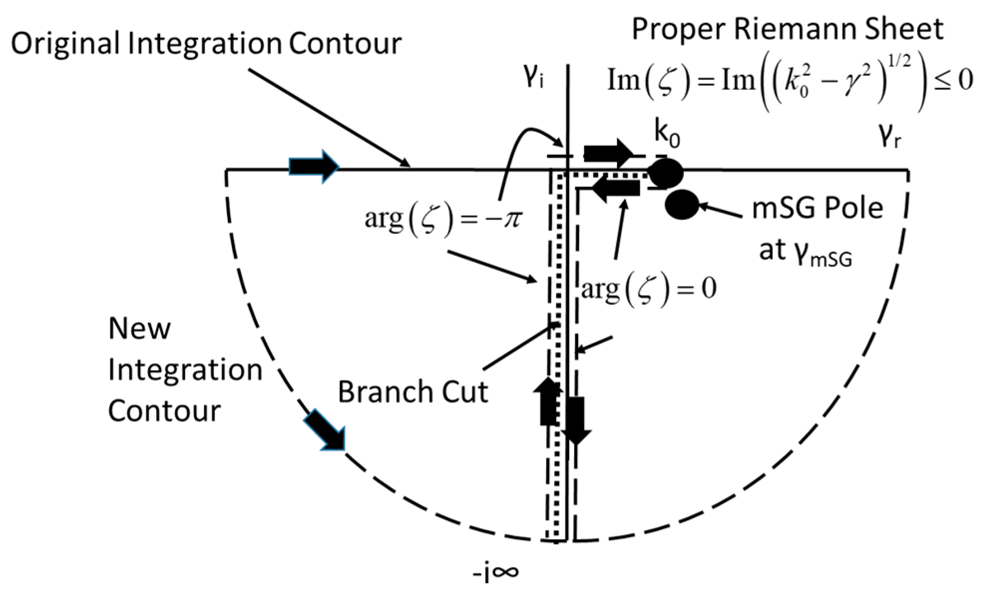
First, (30) for the common mode will be evaluated. In this case, (i.e., Figure 2), the solution will be the branch cut integration plus the residue of a pole ${\gamma }_{mSG}$, which corresponds to the SG pole described in [22] modified by the presence of the second wire.

The result is quite similar to the case discussed in [22], except that the details of the branch cut integration and the mSG mode are different. Also note that if the conductivity becomes infinite, the mSG pole will disappear into the branch cut at $k_0$. One consequence is the more complicated branch cut integration due to the additional term containing the distance d.

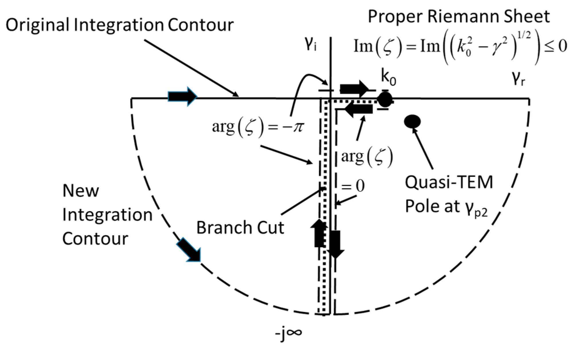
The case for the differential mode is somewhat different, as illustrated in Figure 3. Here, there is no pole that corresponds to the SG pole in the case of a single wire. This can be illustrated through an examination of the denominator of (30). In the single-wire case, there is only a single Hankel function, and the SG pole occurs because this function has a logarithmic singularity near $k_0$. In the case of the two-wire differential mode, the second Hankel function cancels this singularity, and there is no mSG pole. However, there is another pole that corresponds to the well-known quasi-TEM mode for a pair of parallel wires.

3.1. Calculation of Pole Locations

The zero of (31) (i.e., either the mSG or quasi-TEM pole of the integrand of (30) here given as γ_p and known to be near k₀) can be found using Newton’s iterative method. In this case, an initial guess for the zero is selected as γ_p(0) and successive approximations are found as 0028

$${\gamma }_{p(n)}={\gamma }_{p(n-1)}-\frac{{\tilde{D}}_{\pm }({\gamma }_{p(n-1)})}{{{\tilde{D}}_{\pm }}^{\prime }({\gamma }_{p(n-1)})}$$

(34)

where ${\tilde{D}}_{\pm }\left(\gamma \right)$ is given as (31), and its derivative with respect to γ, ${{\tilde{D}}_{\pm }}^{\prime }\left(\gamma \right)$ can be shown to be [24]

$$\begin{array}{l}{{\tilde{D}}_{\pm }}^{\prime }\left(\gamma \right)=-\gamma [-2H_0^{\left(2\right)}\left(\zeta a\right)\mp 2H_0^{\left(2\right)}\left(\zeta d\right)\\ \hspace{1em}\hspace{1em}\hspace{1em}+\zeta a{H}_1^{\left(2\right)}\left(\zeta a\right)\pm \zeta d{H}_1^{\left(2\right)}\left(\zeta d\right)]\end{array}$$

(35)

It has been found that the sequence (34) converges quickly if the initial value γ_p(0) is selected to be near k₀.

A good approximation for the quasi-TEM mode propagation constant (using small argument expansions for the Hankel function in (31) with the minus sign) is

$${\gamma }_{QTEM}\cong k_0-\frac{j\pi {\delta }_{iw}}{4k_0\ln (d/a)}$$

(36)

3.2. Evaluation of the Current

Given the singularities of ${\tilde{D}}_{\pm }\left(\gamma \right)$, (30) can now be evaluated by deforming the original contour around the lower branch cut entirely on the proper Riemann sheet, as illustrated in Figure 2 and Figure 3. Given factor $e^{-j\gamma z}$ in the integrand of (30), the integrations along the lower infinite semicircle are zero. Hence, the original integrations reduce to integrations along both sides of the branch cut, as shown. However, because the pole at γ_p is enclosed by the original and new contours, its residue must be added to each integration.

Equation (30) is integrated around the branch cut using the identities [24]

$$H_0^{\left(2\right)}\left(-z\right)=-H_0^{\left(1\right)}\left(z\right)$$

(37)

$$H_0^{\left(1\right)}\left(\zeta a\right)=J_0\left(\zeta a\right)+j{Y}_0\left(\zeta a\right)$$

(38)

$$H_0^{\left(2\right)}\left(\zeta a\right)=J_0\left(\zeta a\right)-j{Y}_0\left(\zeta a\right)$$

(39)

where $H_0^{\left(1\right)}\left(q\right)$, $J_0(q)$and $Y_0(q)$ are, respectively, the Hankel function of the first kind and Bessel functions of the first and second kind or order zero and argument q. After multiplying the numerator and denominator by ${\zeta }^2$ to avoid infinity in the denominator at $\gamma =k_0$, the horizontal portion of the branch cut integral between 0 and k₀ is (Note that the integrations on the two sides of the branch cut do not cancel because the argument of ζ is different on the each side due to the fact that it is defined as a square root. More specifically, the different arguments of ζ are indicated in Figure 2 and Figure 3).

$${\widehat{I}}_h^{c/d}(z)=\frac{-4\omega {\epsilon }_0\widehat{V}}{\pi }{\displaystyle \underset{0}{\overset{k_0}{\int }}\left(\frac{{\zeta }^2\left(J_0(\zeta a)\pm J_0(\zeta d)\right)e^{-j\gamma z}d\gamma }{M_{\pm }^h\left(\gamma \right)}\right)}$$

(40)

where

$$\begin{array}{l}{M}_{\pm }^h\left(\gamma \right)={\zeta }^4\left({\left(J_0(\zeta a)\pm J_0(\zeta d)\right)}^2+{\left(Y_0(\zeta a)\pm Y_0(\zeta d)\right)}^2\right)\\ \hspace{1em}\hspace{1em}\hspace{1em}+j(2{\delta }_{iw}{\zeta }^2)\left(Y_0(\zeta a)\pm Y_0(\zeta d)\right)-{\delta }_{iw}^2.\end{array}$$

(41)

The vertical portion of the branch cut integral from γ = −j∞ to γ = 0 can be written (after using the substitutions $\gamma =-ju$, $d\gamma =-jdu$) and defining ${\zeta }_i={\left(k_0^2+u^2\right)}^{1/2}$ as

$${\widehat{I}}_v^{c/d}(z)\frac{-j4\omega {\epsilon }_0\widehat{V}}{\pi }{\displaystyle \underset{0}{\overset{\infty }{\int }}\left(\frac{{\zeta }_i^2\left(J_0({\zeta }_{i}a)\pm J_0({\zeta }_{i}d)\right)e^{-uz}du}{M_{\pm }^v\left(\gamma \right)}\right)}$$

(42)

where

$$\begin{array}{l}{M}_{\pm }^v(\gamma )={\zeta }_i^4\left({\left(J_0({\zeta }_{i}a)\pm J_0({\zeta }_{i}d)\right)}^2+{\left(Y_0({\zeta }_{i}a)\pm Y_0({\zeta }_{i}d)\right)}^2\right)\\ \hspace{1em}\hspace{1em}+j(2{\delta }_{iw}{\zeta }_i^2)\left(Y_0({\zeta }_{i}a)\pm Y_0({\zeta }_{i}d)\right)-{\delta }_{iw}^2\end{array}$$

(43)

The subscripts “h” and “v” in (40) and (42) indicate the contribution from the horizontal and vertical portions of the branch cut integration, respectively. If ${\delta }_{iw}$ is finite, (40) and (42) are relatively straightforward to integrate numerically.

As noted earlier in Figure 2 and Figure 3, there is a pole on the proper Riemann sheet in the common mode case (i.e., the mSG pole) and in the differential mode case (i.e., the Quasi-TEM pole) located between the original contour and integration contour used in this work. Hence, the appropriate residue must be added to the branch cut integral in each case. This residue can be found directly from (31) by expanding ${\tilde{D}}_{\pm }\left(\gamma \right)$ as a Taylor series around ${\gamma }_p$. The result is

$${\widehat{I}}_{res}\left(z\right)=\frac{-2\pi j{N}_V}{{\tilde{D}}_{\pm }^{\prime }\left({\gamma }_p\right)}{e}^{-j{\gamma }_{p}z}$$

(44)

where $D_{\pm }^{\prime }\left({\gamma }_p\right)$ can be found in (35).

The total induced modal currents then are

$${\widehat{I}}^c(z)={\widehat{I}}_h^c(z)+{\widehat{I}}_v^c(z)+{\widehat{I}}_{res}^{mSG}(z)$$

(45)

for the common mode and

$${\widehat{I}}^d(z)={\widehat{I}}_h^d(z)+{\widehat{I}}_v^d(z)+{\widehat{I}}_{res}^{QTEM}(z)$$

(46)

for the differential mode.

3.3. The Special Case for Perfectly Conducting Conductors

In the case of ${\delta }_{iw}=0$, the term $1/{\zeta }^2$ in the denominator of (40) and (42) grows without bound near $k_0$ (due to the fact that the pole has been absorbed into k₀). However, in the common mode case, (39) is still integrable since the sum of Neumann functions in the denominator limits this growth. However, more care must be used to evaluate the integral. Note that this does not happen in the differential mode case because the difference in Neumann functions does not grow near k₀. Given this difficulty, (40) is separated into two parts.

$${\widehat{I}}_h^c(z)={\widehat{I}}_{ha}^c(z)+{\widehat{I}}_{hb}^c(z)$$

(47)

where the first is

$$\begin{array}{l}{\widehat{I}}_{ha}^c\left(z\right)=\frac{-4\omega {\epsilon }_0\widehat{V}}{\pi }\cdot \\ \hspace{1em}{\displaystyle \underset{0}{\overset{k_0(1-\Delta )}{\int }}\left(\frac{\left(J_0(\zeta a)+J_0(\zeta d)\right)e^{-j\gamma z}d\gamma }{{\zeta }^2\left({\left(J_0(\zeta a)+J_0(\zeta d)\right)}^2+{\left(Y_0(\zeta a)+Y_0(\zeta d)\right)}^2\right)}\right)}\end{array}$$

(48)

and the second (following the method of [22]) is

$${\widehat{I}}_{hb}^V(z)\cong \frac{-\widehat{V}}{{\eta }_0}{e}^{-j{k}_{0}z}\left\{{\tan }^{-1}\left[\frac{\ln (e^{2{\gamma }_e}{k}_0^{2}ad\Delta /2)}{\pi }\right]+\pi /2\right\}$$

(49)

${\eta }_0=\sqrt{{\mu }_0/{\epsilon }_0}$ is the impedance of free space, γ_e is the Euler constant, Δ is small enough that ${\zeta }^2=\left(k_0^2-{\gamma }^2\right)\cong 2k_0(k_0-\gamma )$ and small argument approximations can be used for the Bessel functions [24]. In this solution, the substitutions $u=(k_0-\gamma )$ and $v=\ln \left(e^{2{\gamma }_e}{k}_0{a}^{2}u\right)$ have been used. Note that (49) accounts for the mSG pole residue, which (for ${\delta }_{iw}=0$) has been absorbed into $k_0$. Finally, (42) along the vertical portion of the branch cut (but with ${\delta }_{iw}=0$) can be evaluated numerically as earlier.

Since the pole at ${\gamma }_p$ is absorbed into k₀, there is no separate residue term. Given these results, the current induced on a perfect conductor by the voltage source is

$${\widehat{I}}_h^c(z)={\widehat{I}}_{ha}^c(z)+{\widehat{I}}_{hb}^c(z)+{\widehat{I}}_v^c(z)$$

(50)

3.4. Relationship to Dipole Excitation

It was shown in [22] that there is a simple relationship between the current excited by a voltage source and that by a dipole in the immediate proximity of the conductor. To convert from the voltage source solution to that for a dipole with current ${\widehat{I}}_d(\omega )$ and length $d\mathcal{l}$ with its center at a distance $d\mathcal{l}/2$ from the outer surface of the conductor, one must multiply the voltage solution by the factor

$$-{\widehat{I}}_d(\omega ){\eta }_0/(V\pi )$$

(51)

Since the dipole is assumed to be very close to the conductor, its influence is limited to that of that conductor in its proximity. Hence, this factor can also be used to convert the two-wire case for a voltage source on one conductor only to the dipole solution for the two-wire case.

3.5. A Simple Solution

Shen, Wu and King [25] have developed a simplified solution for the total current in the single conductor perfectly conducting the case that is valid for $z/(k_0{a}^2)>>1$. It is

$${\widehat{I}}^{cA}(z)\cong \frac{-jV}{{\eta }_0}\ln \left[1+\frac{2\pi j}{\left(\ln (2z/(k_0{a}^2)-{\gamma }_e-j3\pi /2\right)}\right]e^{-j{k}_{0}z}$$

(52)

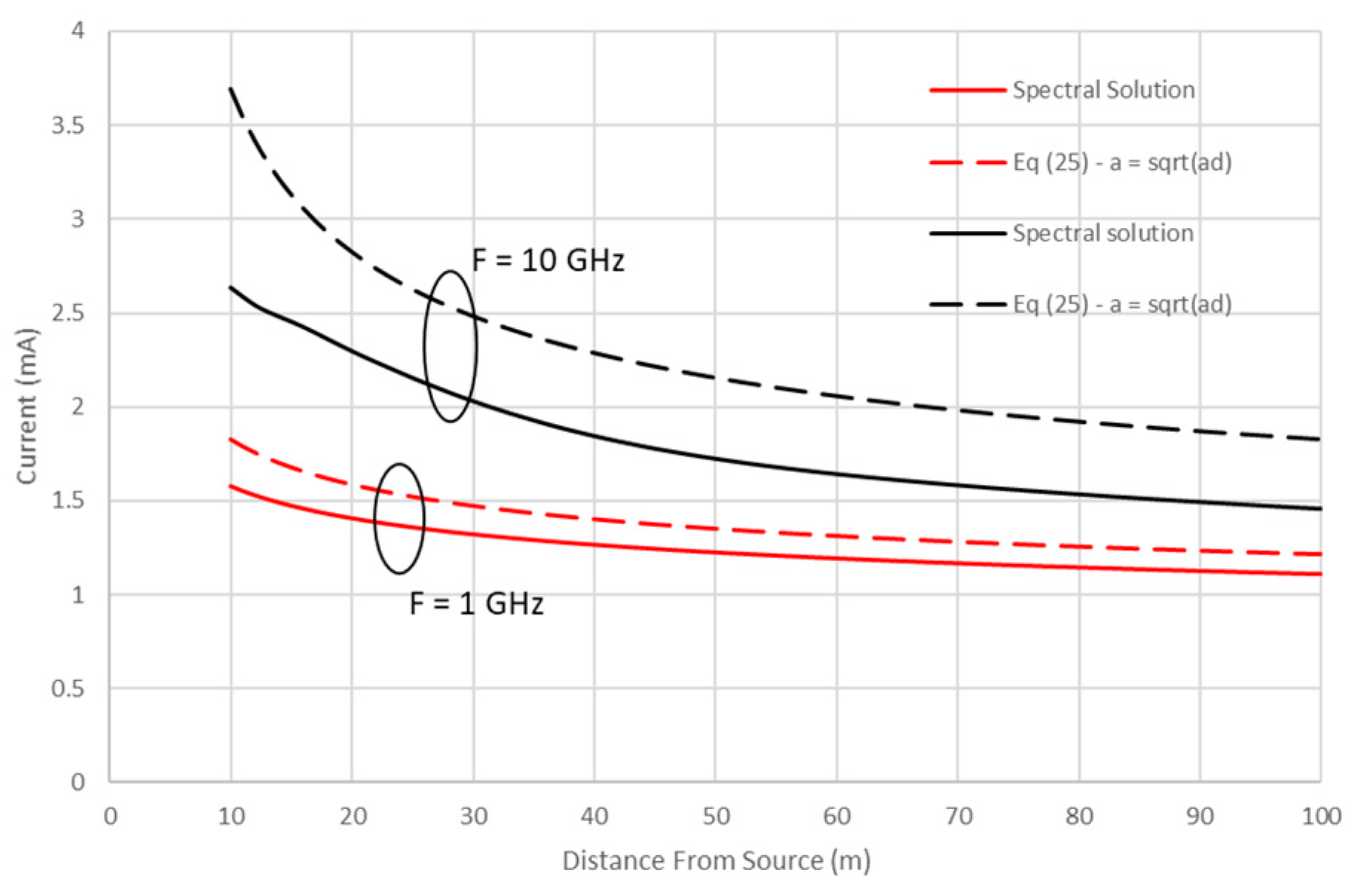
It was shown in [22] that (52) is a very good approximation of the total current (i.e., continuous spectrum plus the SG mode) induced on a conductor with typical conductivity. Hence, it was used as a simple approximation for the total current on a lossy wire. It will be shown in the next section that it is reasonable to use (52) for the common mode current in the two-wire case if the wire radius “a” is replaced by the geometric mean radius of the two wires, $\sqrt{ad}$. The notion that this is reasonable can be shown by examining (49) and noting that a major contribution to the common mode current is the same as that for the single wire case in [22} but with “a” replaced by $\sqrt{ad}$.

It will also be demonstrated shortly that the quasi-TEM mode contribution to the differential mode is the dominant contribution away from the immediate vicinity of the source. Its residue (using small argument expansions for the Hankel functions in (35) is

$${\widehat{I}}^{dA}(z)=\frac{2\pi V}{{\eta }_0\ln (d/a)}{e}^{-j{\gamma }_{QTEM}z}$$

(53)

Hence, a reasonable approximation for the total current on the two wires is as follows

$${\widehat{I}}_{1/2}(z)={\widehat{I}}^{cA}(z)\pm {\widehat{I}}^{dA}(z)$$

(54)

where the plus (minus) sign is for the current on wire one (two).

4. Results

4.1. Pole Locations

The first result (shown in

Table 1. Modal propagation constants for a = 1 cm, σ_w = 3.5 × 10⁷ S/m, d (for mSG and Quasi-TEM) = 0.5 m.

Frequency (GHz)	Type of Pole	$({\mathit{\gamma }}_{\mathit{p}}-{\mathit{k}}_0)/{\mathit{k}}_0 \times {10}^{-6}$
1	SG	9.1 − j10.3
1	mSG	5.9 − j7.0
1	Quasi-TEM	17.2 − j17.2
10	SG	3.8 − j4.5
10	mSG	2.8 − j3.7
10	Quasi-TEM	5.5 − j5.6

) is a set of propagation constants for the SG (single wire) mode discussed in [22] and the mSG (two-wire common) and quasi-TEM (differential) modes for 1 and 10 GHz. The SG and mSG modes were found using a numerical solution of (31) set to zero without (for the SG mode) and with (for the mSG mode assuming the + sign) the second Hankel function. The quasi-TEM pole location has been determined using (31) set to zero with a minus sign or (36).

It is clear that the mSG mode has slightly less loss than the SG mode. This is due to the fact that the current is spread out over a larger area of wire surface. However, the Quasi-TEM mode has a significantly larger loss factor. Hence, for communication systems, it is important to examine the excitation of each mode in the single- and two-wire cases.

4.2. Common vs. Differential Mode Solutions

In Figure 4, results are shown for the magnitude of the current distributions at 1 GHz for the common and differential modes. Two methods are used for calculating the common mode current: the perfect conducting method of (47) and the lossy conductor case in (45). There is little difference between these two methods over typical communication ranges, as was the case in [22]. Hence, perfect conductor theory can be used. Second, in the lossy conductor case, both the continuous spectrum and the mSG modal component are important for typical communication distances. There is no important condition (for communications) for which the mSG mode dominates the continuous spectrum (at least for the source studied here). Note, however, that for the differential mode, the quasi-TEM mode dominates even at very short distances away from the source.

Figure 5 illustrates that (52) is a reasonable approximation for the total common mode current, (44), with $a\to \sqrt{ad}$, especially at lower microwave frequencies. When this substitution is made, the branch cut integration of (40)–(43) can be avoided.

Figure 6 and Figure 7 are plots of the individual wire currents excited by a voltage generator at z = 0 on wires 1 and 2, as well as the single wire current from [22] for frequencies of 1 and 10 GHz, respectively. As expected, the current on wire 1 exceeds that on wire 2 in the two-wire case. In addition, of interest is the fact that the current on wire 1 at 100 m for the two-wire case is significantly higher than that on the single wire. This indicates that the performance of a microwave power line communication system can be enhanced by the existence of parallel wires. This conclusion is consistent with that reported in [7]. Additionally, when approximations of (52)–(54) can be used, very simple expressions for the current result. This is more commonly true for ${\widehat{I}}_1(z)$, which has smaller errors and is also more important for evaluating communication systems.

4.3. Communication System Performance

It was shown in [22] that there are significant advantages to using a power line conductor as an open waveguide compared to free space communication systems for microwave communications links between two power line poles on the order of 100 m apart. Because the total attenuation of a system containing two conductors is smaller than that for a single conductor, this conclusion is even stronger than the two-wire case.

5. Conclusions

• Closed-form solutions for the common and differential mode currents excited on a pair of parallel wires by a voltage source on one wire have been derived. Spectral solutions using a continuous spectrum of currents and the modified Sommerfeld–Goubau (mSG) and quasi-TEM modes in the common and differential mode cases, respectively, are given.
• It is shown that the mSG mode is not the primary reason why microwave communication using power line conductors for distances on the order of 100 m has relatively small losses.
• A simple formula for the total current on the driven wire may often be used to approximate the total induced current in the two-wire case.
• For distances comparable to microwave power line communication system repeater spacing, using power line conductors as a waveguide has significant advantages over free space communications. Further, a second conductor can enhance system performance.