Abstract
The global demand for energy has been steadily increasing due to population growth, urbanization, and industrialization. Numerous researchers worldwide are striving to create precise forecasting models for predicting energy consumption to manage supply and demand effectively. In this research, a time-series forecasting model based on multivariate multilayered long short-term memory (LSTM) is proposed for forecasting energy consumption and tested using data obtained from commercial buildings in Melbourne, Australia: the Advanced Technologies Center, Advanced Manufacturing and Design Center, and Knox Innovation, Opportunity, and Sustainability Center buildings. This research specifically identifies the best forecasting method for subtropical conditions and evaluates its performance by comparing it with the most commonly used methods at present, including LSTM, bidirectional LSTM, and linear regression. The proposed multivariate, multilayered LSTM model was assessed by comparing mean average error (MAE), root-mean-square error (RMSE), and mean absolute percentage error (MAPE) values with and without labeled time. Results indicate that the proposed model exhibits optimal performance with improved precision and accuracy. Specifically, the proposed LSTM model achieved a decrease in MAE of 30%, RMSE of 25%, and MAPE of 20% compared with the LSTM method. Moreover, it outperformed the bidirectional LSTM method with a reduction in MAE of 10%, RMSE of 20%, and MAPE of 18%. Furthermore, the proposed model surpassed linear regression with a decrease in MAE by 2%, RMSE by 7%, and MAPE by 10%.These findings highlight the significant performance increase achieved by the proposed multivariate multilayered LSTM model in energy consumption forecasting.
1. Introduction
Energy consumption refers to the amount of energy used over a certain period of time, typically measured in kilowatt-hours (kWh) or British thermal units (BTUs). It is a crucial metric for evaluating energy usage, efficiency, and understanding the energy requirements of a specific region or country [1]. Urban mining, which involves extracting valuable minerals from waste or secondary resources, is emphasized as a sustainable solution. Various secondary resources, such as biomass, desalination water, sewage sludge, phosphogypsum, and e-waste, have been evaluated for their market potential and elemental composition, showcasing their potential to partially replace minerals in different sectors. The review also discusses technological advancements in mineral extraction from waste, emphasizing the importance of improving processes for large-scale implementation [2]. In the context of renewable energy, biofuels are identified as a potential alternative for the transportation industry, and research on utilizing surplus rice straw as a feedstock for biofuels is explored. While biofuels have the potential to reduce emissions, further research is needed to address concerns regarding food security, feedstock selection, and their impact on climate and human health [3].
According to the International Energy Agency (IEA) [4], global energy consumption is expected to continue to increase in the coming decades, driven by population growth, urbanization, and industrialization in developing countries. However, most of the current research has focused on forecasting for countries or regions [5,6]. There are only a limited number of studies that specifically focus on forecasting for individual buildings. Energy consumption in buildings encompasses the precise measurement of energy utilized for specific purposes such as heating, cooling, lighting, and other essential functions within residential, commercial, and institutional structures. In China and India, buildings account for 37% [7] and 35% [8] of global energy consumption, making it an important area for energy efficiency and sustainability efforts [9].
In this study, we propose a forecasting model for energy consumption for various commercial buildings, such as Hawthorn Campus—ATC Building, Hawthorn Campus—AMDC Building, Wantirna Campus—KIOSC Building. In the study, the proposed model, along with its trained data preprocessing method, demonstrated superior performance compared with other popular models, particularly when there is a sufficient amount of training data available or when there is a lack of training data. The results indicate that the proposed method and model can be used to accurately predict energy consumption in commercial buildings, which is crucial for energy management and conservation. In addition, the proposed method can be easily applied to other commercial buildings with similar energy consumption patterns, providing a practical solution for energy management in the commercial building sector.
The rest of this study is organized as follows. Section 2 presents background knowledge by reviewing the existing research on forecasting models and their adoption for energy consumption forecasting. Section 3 introduces the available data and the configuration of the experiment. Section 2 provides the background of the research. Section 4 provides the details of the proposed model. Section 5 describes some popular bench-marking models. Section 6 presents the experiment to evaluate the efficiency of the models on different datasets. Finally, the conclusion of this study is given in Section 7.
2. Background
2.1. Forecasting Models
A forecasting model is a mathematical algorithm or statistical tool used to predict future trends, values, or events based on historical data and patterns. A forecasting model M that analyzes the historical values from the current time to return the predicted future value at time (denoted as ) is built. The objective of the forecasting model is to minimize the discrepancy between the estimated value and the actual value by seeking the closest approximation. To achieve this in a temporal context where data points are indexed in time order, a specific type of forecasting model is often used.
A time series forecasting model is a predictive algorithm that utilizes historical time-series data to anticipate future trends or patterns in the data over time. Two techniques are available for building the model M to obtain this objective, i.e., (i) univariate and (ii) multivariate time-series (TS) [10,11,12]. In univariate TS, only a 1D sequence of energy consumption value is utilized to produce the estimated value , where k is a period of time from the current time [13,14]. By contrast, for multivariate TS, we could employ one or more other historical features in addition to the energy consumption for training model M [15]. They can be time fields or other specific sources. Therefore, the input for multivariate TS is a multi-dimensional sequence , with is a vector of dimension n. In forecasting new values, the model could be enhanced if related available features are taken into account. The additional information could help the model capture the dependencies or correlations between features and the target variable. Therefore, the model could better understand the context, mitigate the impact of missing values, and make more precise predictions. Therefore, multivariate TS has been frequently employed for building the forecasting model recently [16].
2.2. Energy Consumption Forecasting
Energy consumption forecasting refers to predicting a particular region’s future energy consumption based on historical consumption and other relevant factors [1]. Accurate energy consumption forecasting is essential for proper energy planning, pricing, and management. It plays a significant role in the transition toward a more sustainable energy future. There have been numerous studies on energy consumption forecasting, and various models have been proposed for this purpose [17]. As shown in Figure 1, in the literature, forecasting models often fall into two categories: (i) Conventional Models and (ii) Artificial Intelligence (AI) Models. Table 1 shows different forecasting models for commercial buildings. It shows the names of forecasting techniques, locations, and performance evaluation indexes with the best accuracy.
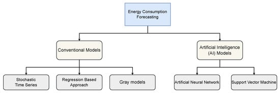
Figure 1.
Common categories of Forecasting model in the literature.

Table 1.
Summary of different forecasting models for commercial buildings.
Conventional models used in energy consumption forecasting commonly include Stochastic time series (TS) models [30], regression models (RMs) [31], and gray models (GMs) [32,33]. These models typically require historical energy consumption data as input and use various statistical and mathematical techniques to make future energy consumption predictions. However, these models may not be able to capture complex nonlinear relationships and may require manual feature engineering, making them less efficient and scalable compared with AI-based models. AI-based models have become increasingly popular in the field of energy forecasting due to their ability to learn patterns and relationships in complex data [34,35,36]. The use of AI in energy forecasting has the potential to reduce energy costs, optimize energy production, and enhance energy security. Furthermore, LSTM models are able to capture both short-term and long-term dependencies in TS data. They are also capable of handling non-linear relationships between input and output variables, which is important in energy forecasting, where the relationships may be complex. Finally, LSTMs could process sequential data of varying lengths, which is useful for handling variable-length TS data in energy forecasting.
3. Data Used in This Study
3.1. Data Collection
Data collected from three buildings in different regions is employed to evaluate the models, i.e., Hawthorn Campus—ATC Building (denoted as ), Hawthorn Campus—AMDC Building (denoted as ), and Wantirna Campus—KIOSC Building (denoted as ) are incredibly valuable as it provides real-time insights into the building’s performance, energy consumption, and operational efficiencies, allowing for a swift response to potential issues. This real-time data not only enhance decision-making capabilities for building management, maintenance, and optimization but also provides a basis for developing more accurate forecasting models. Furthermore, it can guide strategic energy management, potentially leading to significant cost savings, improved sustainability, and increased occupant comfort over time. The two datasets and contain the energy consumption from 2017 to 2019, and the dataset contains the energy consumption from 2018 to 2019. The prediction value is the difference between the previous and the intermediate next time in using energy, or the cumulation of energy. The historical value is 96 data points every 15 min to predict the next value. Figure 2 Indicates the location of the buildings from the Hawthorn Campus and the Wantrina Campus in the context of Melbourne and Figure 3 and Figure 4 indicate the Electricity accumulation in every 15 min and one hour for the Hawthorn campus (ATC building).
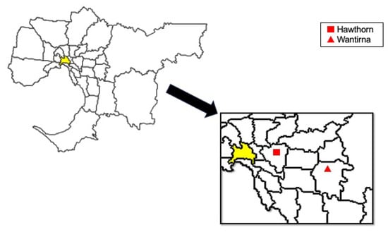
Figure 2.
Location of Hawthorn Campus and Wantirna Campus in Metropolitan Melbourne, Victoria, Australia.
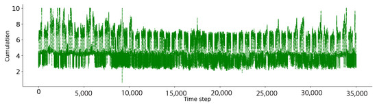
Figure 3.
Electricity accumulation in every 15 min at Hawthorn Campus—ATC Building.
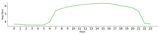
Figure 4.
Average electricity accumulation in every 1 h at Hawthorn Campus—ATC Building in 2018. As can be seen, electricity consumption peaks between 8 a.m. and 21 p.m.
3.2. Data Setup
Dataset. In this experiment, three datasets from three buildings in different regions are employed to evaluate the models, i.e., Hawthorn Campus—ATC Building (denoted as ), Hawthorn Campus—AMDC Building (denoted as ), and Wantirna Campus—KIOSC Building (denoted as ). The two datasets and contain the energy consumption from 2017 to 2019, and the dataset contains the energy consumption from 2018 to 2019. The prediction value is the difference between the previous and the intermediate next time in using energy, or the cumulation of energy. The historical value is 96 data points every 15 min to predict the next value.
Configuration of the proposed model. The proposed model, , consists of a succession of one input layer, two LSTM layers, and one dense layer at the end. The input layer contains two input types, as described in Section 4.1. In the following, the first LSTM layer wraps eight LSTM units, and the second wraps four units. The last dense layer has one unit for predicting energy consumption.
Configuration of bench-marking models. As mentioned earlier, three competitive models are used for comparison: LSTM, Bi-LSTM, LR, and SVM models. The LSTM model consists of one single layer with one unit, followed by a Dense layer for prediction. The Bi-LSTM consists of one single Bi-Directional LSTM layer of one unit, followed by a Dense layer for prediction as the LSTM model. The LR model trains on one dense layer.
Training Configuration. Both , LSTM, Bi-LSTM, LR, and SVM models are trained using the same training set and evaluated on the same test set. In and , the models are trained on the data from 2017 and 2018. In , the models are trained on the data from 2018 to demonstrate the ability of models with a lack of training data.
4. Methodology
In this section, we propose the forecasting model (Multivariate Multilayered LSTM), which is referred to as . The overview of the proposed method is illustrated in Figure 5. There are three phases, i.e., data preprocessing, model training, and evaluation.
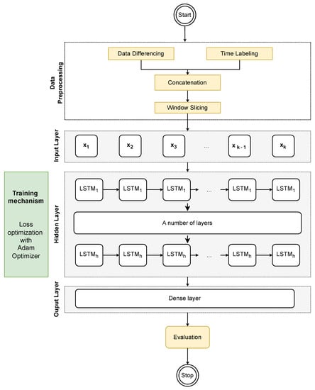
Figure 5.
Workflow of the proposed model.
4.1. Data Preprocessing
Two major techniques are used in the data preprocessing phase, i.e., (i) data differencing and (ii) time labeling. Additionally, there are two other techniques, i.e., (iii) concatenation and (iv) window slicing.
In regard to data differencing, due to a large amount of energy consumption and the fact that the value is not commonly stationary, the difference between the data value and its previous data value is taken into account. By removing these patterns through data differencing, the resulting stationary TS can be more easily modeled and forecasted. This technique is often required for many forecasting models [37].
In time labelling, the amount of energy consumed during peak time points is typically greater than that during non-peak times. Consequently, the labeling convention assigns a value of 1 to peak time and 0 to non-peak time [38]. These labeled time periods serve as valuable features for training the forecasting model. In the concatenation phase, the data from data differencing and labeled time are concatenated and then sliced into vectors with a length of k during the window-slicing phase.
4.2. Forecasting Model—Multivariate Multilayered LSTM
is an extension of the LSTM model, which is a type of recurrent neural network (RNN) architecture used for sequential data processing tasks such as TS forecasting. There are h sub-layers In the hidden layer. The model consists of multiple LSTM layers, with each layer having its own set of neurons that process the input variables independently. The output of each layer is then fed into the next layer, allowing the model to capture more complex and abstract relationships between the input variables. There are some additional layers, such as the dropout layer, normalization layer, etc., in the hidden part for training the model efficiently.
As shown in Figure 6, the memory cell is responsible for storing information about the long-term dependencies and patterns in the input sequence, while the gates control the flow of information into and out of the cell. The gates are composed of sigmoid neural network layers and a point-wise multiplication operation, that allows the network to learn which information to keep or discard. In particular, each ith cell at the layer m, denoted as , has three inputs, i.e., the hidden state , cell state of the previous cell, and the hidden state of the cell i at the previous layer . The cell has two recurrent features, i.e., hidden state , and cell state . is a mathematical function as Equation (1), that takes three inputs and returns two outputs. Both outputs leave the cell at time i and are fed into that same cell at time , and the input sequence is also fed into the cell. In the first layer (), the hidden state is the input .
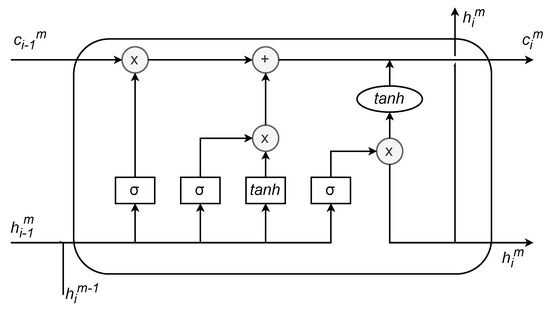
Figure 6.
Illustration of the ith LSTM cell at the layer m.
Inside the ith cell, the previous hidden state and input vector are fed into three gates. i.e., input gate (), forget gate (), output gate (). They are functions (), each of which produces a scalar value as described in Equations (2)–(4) respectively.
where and denote weight, which is the parameter that should be updated during the training of the cell. Another scalar function, called the update function (denoted as ) has a activation function as described in Equation (5).
where and are further weighted to be learned. The returned cell state () and hidden state () are formulated in Equation (6), (7) respectively.
In energy forecasting, loss optimization is one of the important steps to improve the accuracy of the model [39]. One common technique for loss optimization is using the Adam optimizer, which is a stochastic gradient descent optimizer that uses moving averages of the parameters to adapt the learning rate. The Adam optimizer computes individual adaptive learning rates for different parameters from estimates of the first and second moments of the gradients. This makes it suitable for optimizing the loss function in models where there are a large number of parameters. By using the Adam optimizer, the model can efficiently learn and update the weights of the neurons in each time step, resulting in better prediction accuracy. In addition, the loss function formulation of the Adam optimizer used in the proposed model aims to strike a balance between accuracy and robustness, taking into account the unique characteristics of the data and the specific requirements of the forecasting task.
5. Bench-Marking Models
In this study, we compare the proposed model with three well-known models, i.e., linear regression (LR), long-short-term memory (LSTM), bidirectional long-short-term memory (Bi-LSTM), and Support Vector Machine (SVM).
5.1. Linear Regression
LR allows knowing the relationship between the response variable (energy consumption) and the return variables (the other variables). As a causative technique, regression analysis predicts energy demand from one or more reasons (independent variables), which might include things such as the day of the week, energy prices, the availability of housing, or other variables. When there is a clear pattern in the previous forecast data, the LR method is applied. Due to this, its simple application has been used in numerous works related to the prediction of electricity consumption. Bianco V et al. (2009) used a LR model to conduct a study on the projection of Italy’s electricity consumption [40], while Saab C et al. (2001) looked into various univariate modeling approaches to project Lebanon’s monthly electric energy usage [41]. With the help of our statistical model, this research has produced fantastic outcomes.
The LR model works by fitting a line to a set of data points with the goal of minimizing the sum of the squared differences between the predicted and actual values of the dependent variable. The slope of the line represents the relationship between the dependent and independent variables, while the intercept represents the value of the dependent variable when the independent variable is equal to zero. The LR model describes the linear relationship between the previous values and the estimated future value , formulated as follows:
5.2. LSTM
The LSTM technique is a type of Recurrent Neural Network (RNN). The RNNs [42] are capable of processing data sequences, or data that must be read together in a precise order to have meaning, in contrast to standard neural networks. This ability is made possible by the RNNs’ architectural design, which enables them to receive input specific to each instant of time in addition to the value of the activation from the previous instant. Given their ability to preserve data from earlier actions, these earlier temporal instants provide for a certain amount of “memory”. Consequently, they possess a memory cell, which maintains the state throughout time [43]. Figure 7 illustrates an overview of the simple LSTM Model.
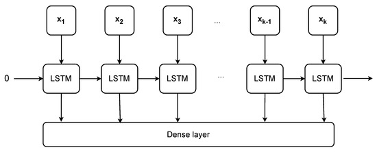
Figure 7.
Overview of the LSTM model.
As noted in Section 4, the LSTM [44] model has the ability to remove or add information to decide what information needs to go through the network from the cell state [44]. Different from the model, the LSTM model has just one LSTM layer, with the input sequence . Therefore, the hidden state (h) and cell state (c) for the ith LSTM cell are calculated as Equation (9).
In the experiment, we compare the performance of the proposed model with the univariate and multivariate LSTM models. The univariate LSTM takes the first input (i) described in Section 4.1, and the multivariate LSTM takes both those inputs.
5.3. Bidirectional LSTM
Bi-LSTM is also an RNN. It utilizes information in both the previous and following directions in the training phase [45]. The fundamental principle of the Bi-LSTM model is that it examines a specific sequence from both the front and back. Which uses one LSTM layer for forward processing and the other for backward processing. The network would be able to record the evolution of energy that would power both its history and its future [46]. This bidirectional processing is achieved by duplicating the hidden layers of the LSTM, where one set of layers processes the input sequence in the forward direction and another set of layers processes the input sequence in the reverse direction. As illustrated in Figure 8, the hidden state () and the cell state () in the ith forward LSTM cell are calculated as similar as the Equation (9). On the contrary, each LSTM cell in the backward LSTM takes the following hidden state (), and following cell state (), and as input. Therefore, the hidden state () and cell state () of the ith backward LSTM cell are calculated as Equation (10).
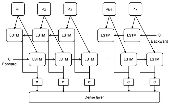
Figure 8.
Overview of the Bi-LSTM model.
After the calculations of both forward and backward LSTM cells, the hidden states of the two directions could be concatenated or combined in some way to obtain the output. The common combination is the sigmoid function, as noted in Figure 8. The output is fed into the Dense layer to obtain the final prediction. Similar to the LSTM model, we also compare the proposed model with univariate and multivariate Bi-LSTM models.
5.4. Support Vector Machine
Support Vector Machines (SVM) are supervised machine learning models used for both classification and regression tasks. In this paper, SVM with a Radial Basis Function (RBF) kernel is used for the regression task. This kind of SVM model utilizes the RBF kernel to transform the input space into a higher-dimensional feature space, enabling the SVM to learn nonlinear decision boundaries. The formulation of the RBF kernel is defined as Equation (11).
where , are input data points, denotes the Euclidean distance between them, and is a parameter that controls the width of the Gaussian curve. Higher values of gamma result in more localized and complex decision boundaries. Furthermore, the decision function in SVM with RBF kernel can be represented as Equation (12).
where, is the input data point, b is the bias term, is the Lagrange multiplier associated with the ith support vector, is the corresponding class label, is the RBF kernel function, and the summation is performed over all support vectors.
The SVM with RBF kernel formulation aims to find the optimal hyperplane that maximizes the margin between the classes while allowing some misclassifications. The RBF kernel enables the SVM to capture complex, nonlinear patterns in the data by mapping the data to a higher-dimensional feature space. The model is trained by solving the quadratic programming problem to find the Lagrange multipliers () and bias term b that define the decision function.
6. Experiment
6.1. Metric
To better evaluate the performance, a model is tested by making a set of predictions and then comparing it with a set of known actual values , where D is the size of the test set. Three common metrics are used to compare the overall distance of these two sets, i.e., mean absolute percentage error (), normalized root mean squared error (), and R-squared score ( score).
MAPE As shown in Equation (13), is calculated by taking the absolute difference between the predicted and actual values, dividing it by the actual value, and then taking the average of these values over the entire dataset. This calculation results in a single number that represents the average percentage difference between the predicted and actual values. The smaller the value, the better the model’s performance
NRMSE Normalized Root Mean Squared Error () is a metric used to evaluate the accuracy of a prediction model. It measures the normalized average magnitude of the residuals or errors between the predicted values and the actual values, as shown in Equation (14).
where, represents the predicted values, A represents the actual values, and denotes the square root function. The term calculates the squared residuals or errors between the predicted and actual values. The and represent the maximum and minimum values in the actual values, respectively. The smaller the value, the better the model’s performance.
score The score, also known as the coefficient of determination, is a statistical measure that indicates the proportion of the variance in the dependent variable that is predictable from the independent variables in a regression model. The score is typically used to evaluate the fitness of a regression model, as formulated in Equation (15).
where the mean of the actual values. In essence, the score is a measure of how well the regression model fits the data and provides an assessment of its predictive performance. A higher score indicates a better fit and stronger explanatory power of the model.
6.2. Result and Discussion
This study aims to experimentally address the effectiveness of the proposed model by answering the following research inquiries: the general performance of training the proposed model and the comparative performance analysis against other competitive models.
6.2.1. General Performance
In the first part of the experiments, is trained and evaluated with two types of data preprocessing strategies, i.e., with a labeled time field and without a labelled time field. Figure 9 shows the results of the test set in , , and . In this question, there are two results, (i) a sufficient training set, and (ii) a lack of a training set.
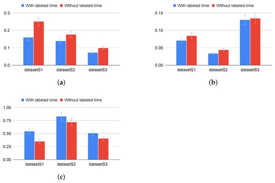
Figure 9.
Comparison of trained with labelled time and without labelled time. (a) error in the scale of (0, 1), (b) error, (c) score. Note that, the higher score indicates the better model’s performance.
For the first result (i), the model is sufficiently trained with data from 2017 and 2018 and evaluated in 2019 from and . Figure 9 shows that the model achieves better performance in all three metrics with the labeled time field. The results are similar under the same settings for the other models. The details are provided in Table 2 and the line plot in Figure 10. Therefore, the models can learn and extract more valuable features if they are trained with the appropriate data preprocessing strategy.
Table 2.
Comparison of with competitive models with and without labelled time. , , score. are denoted metrics for model trained with labelled time. , , score are denoted metrics for model trained without labelled time. and are rescale to the range from 0 to 1. Better values are marked in bold.
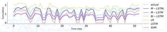
Figure 10.
Comparison of with labelled time () with without labelled time, and other models in case of lack of training data ( in 2019). The time step is 7 days.
For the second result (ii), the model is only trained with data from 2018 and evaluated in 2019 from . Figure 10 shows that the model performed well in predicting and matching the actual values, as evidenced by its superior fit line compared with the other models in Figure 9 and Figure 10. These findings suggest that the proposed preprocessing method is effective, particularly in situations with a limited amount of training data available for model training.
6.2.2. Experience Different Models
In the second part of the experiments, we compare the performance evaluation results of to those of other competitive models (LSTM, Bi-LSTM, LR, and SVM models) on three datasets in terms of three metrics. Two sets of performance metrics are presented; one set includes time label information (, , score), whereas the other set does not include time label information (, , score). Table 2 presents the performance evaluation results of and LSTM, Bi-LSTM, LR, and SVM models on three datasets in terms of three metrics. Figure 11 shows the error of models with and without labeled time.
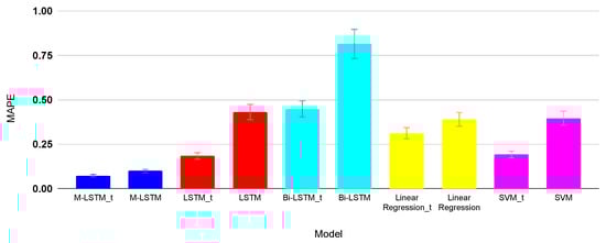
Figure 11.
Bart chart in the comparison of with labelled time () with without labelled time, and other models with and without labelled time in case of lack of training data ( in 2019).
In general, the results indicate that models using labelled time information tend to perform better than those that do not use labelled time information in the same setting. For example, on , the four models get lower values, while the same models have higher error values. On the other hand, among the different models, the model using the labeled time information tends to perform the best overall, with the lowest , , and the highest score in most cases. To summarize, using the proposed preprocessing method with time information tends to improve the performance of the models. The model using time label information performs the best in general. The labeled time field provides useful information for predicting energy consumption in peak and non-peak periods. These findings suggest that considering time information can help in accurately predicting the target variable in the studied datasets.
7. Conclusions
In conclusion, this work presents a method for pre-processing data and a model for accurately predicting energy consumption in commercial buildings, specifically focusing on buildings on the Hawthorn and Wantirna campuses. The proposed pre-processing method effectively improves the accuracy of energy consumption prediction, even when training data are limited. The results demonstrate the applicability of the proposed method and model for accurately predicting energy consumption in various commercial buildings.
The proposed model, denoted as , achieved the lowest values of 0.159, 0.139, and 0.072 for , , and , respectively. This achievement is crucial for effective energy management and conservation in commercial buildings. The practicality of this approach extends to other commercial buildings with similar energy consumption patterns, making it a viable solution for energy management in the commercial building sector. Visualizations were also provided to aid in understanding the data patterns and trends in the model predictions. Additionally, further research can explore the effectiveness of the proposed pre-processing method and models in predicting energy consumption for different types of buildings or larger datasets. Exploring alternative techniques, such as seasonal decomposition or time series analysis, for incorporating time information into the models could also yield valuable insights. These advancements in energy consumption forecasting contribute to significant cost savings and environmental benefits in commercial buildings.
Author Contributions
Individual Contribution: Conceptualization, T.N.D., G.S.T., M.S., S.M. and A.S.; Methodology, T.N.D., G.S.T. and M.S.; Software, T.N.D. and G.S.T.; Validation, M.S., A.S. and S.M.; Formal analysis, G.S.T., M.S., A.S. and S.M.; Investigation, G.S.T., M.S., S.M. and A.S.; Resources, M.S., A.S. and S.M.; Data curation, G.S.T., T.N.D. and M.S.; Writing—original draft preparation, T.N.D. and G.S.T.; Writing—review and Editing, M.S., S.M. and A.S.; Visualization, G.S.T., T.N.D. and M.S. All authors have read and agreed to the published version of the manuscript.
Funding
This research received no external funding.
Institutional Review Board Statement
Not applicable.
Informed Consent Statement
Not applicable.
Data Availability Statement
Not applicable.
Conflicts of Interest
The authors declare no conflict of interest.
References
- Khalil, M.; McGough, A.S.; Pourmirza, Z.; Pazhoohesh, M.; Walker, S. Machine learning, deep learning and statistical analysis for forecasting building energy consumption—A systematic review. Eng. Appl. Artif. Intell. 2022, 115, 105287. [Google Scholar] [CrossRef]
- Agrawal, R.; Bhagia, S.; Satlewal, A.; Ragauskas, A.J. Urban mining from biomass, brine, sewage sludge, phosphogypsum and e-waste for reducing the environmental pollution: Current status of availability, potential, and technologies with a focus on LCA and TEA. Environ. Res. 2023, 224, 115523. [Google Scholar] [CrossRef] [PubMed]
- Alok, S.; Ruchi, A.; Samarthya, B.; Art, R. Rice straw as a feedstock for biofuels: Availability, recalcitrance, and chemical properties: Rice straw as a feedstock for biofuels. Biofuels Bioprod. Biorefining 2017, 12, 83–107. [Google Scholar]
- IEA. Clean Energy Transitions in Emerging and Developing Economies; IEA: Paris, France, 2021. [Google Scholar]
- Shin, S.-Y.; Woo, H.-G. Energy consumption forecasting in korea using machine learning algorithms. Energies 2022, 15, 4880. [Google Scholar] [CrossRef]
- Özbay, H.; Dalcalı, A. Effects of COVID-19 on electric energy consumption in turkey and ann-based short-term forecasting. Turk. J. Electr. Eng. Comput. Sci. 2021, 29, 78–97. [Google Scholar] [CrossRef]
- Ji, Y.; Lomas, K.J.; Cook, M.J. Hybrid ventilation for low energy building design in south China. Build. Environ. 2009, 44, 2245–2255. [Google Scholar] [CrossRef]
- Manu, S.; Shukla, Y.; Rawal, R.; Thomas, L.E.; De Dear, R. Field studies of thermal comfort across multiple climate zones for the subcontinent: India Model for Adaptive Comfort (IMAC). Build. Environ. 2016, 98, 55–70. [Google Scholar] [CrossRef]
- Delzendeh, E.; Wu, S.; Lee, A.; Zhou, Y. The impact of occupants’ behaviours on building energy analysis: A research review. Renew. Sustain. Energy Rev. 2017, 80, 1061–1071. [Google Scholar] [CrossRef]
- Itzhak, N.; Tal, S.; Cohen, H.; Daniel, O.; Kopylov, R.; Moskovitch, R. Classification of univariate time series via temporal abstraction and deep learning. In Proceedings of the 2022 IEEE International Conference on Big Data (Big Data) IEEE, Osaka, Japan, 17–20 December 2022; pp. 1260–1265. [Google Scholar]
- Ibrahim, M.; Badran, K.M.; Hussien, A.E. Artificial intelligence-based approach for univariate time-series anomaly detection using hybrid cnn-bilstm model. In Proceedings of the 2022 13th International Conference on Electrical Engineering (ICEENG) IEEE, Cairo, Egypt, 29–31 March 2022; pp. 129–133. [Google Scholar]
- Hu, M.; Ji, Z.; Yan, K.; Guo, Y.; Feng, X.; Gong, J.; Zhao, X.; Dong, L. Detecting anomalies in time series data via a meta-feature based approach. IEEE Access 2018, 6, 27760–27776. [Google Scholar] [CrossRef]
- Niu, Z.; Yu, K.; Wu, X. Lstm-based vae-gan for time-series anomaly detection. Sensors 2020, 20, 3738. [Google Scholar] [CrossRef]
- Warrick, P.; Homsi, M.N. Cardiac arrhythmia detection from ecg combining convolutional and long short-term memory networks. In Proceedings of the 2017 Computing in Cardiology (CinC) IEEE, Rennes, France, 24–27 September 2017; pp. 1–4. [Google Scholar]
- Karim, F.; Majumdar, S.; Darabi, H.; Harford, S. Multivariate lstm-fcns for time series classification. Neural Netw. 2019, 116, 237–245. [Google Scholar] [CrossRef]
- Gasparin, A.; Lukovic, S.; Alippi, C. Deep learning for time series forecasting: The electric load case. CAAI Trans. Intell. Technol. 2021, 7, 1–25. [Google Scholar] [CrossRef]
- Wei, N.; Li, C.; Peng, X.; Zeng, F.; Lu, X. Conventional models and artificial intelligence-based models for energy consumption forecasting: A review. J. Pet. Sci. Eng. 2019, 181, 106187. [Google Scholar] [CrossRef]
- Kim, Y.; Son, H.G.; Kim, S. Short term electricity load forecasting for institutional buildings. Energy Rep. 2019, 5, 1270–1280. [Google Scholar] [CrossRef]
- Chitalia, G.; Pipattanasomporn, M.; Garg, V.; Rahman, S. Robust short-term electrical load forecasting framework for commercial buildings using deep recurrent neural networks. Appl. Energy 2020, 278, 115410. [Google Scholar] [CrossRef]
- Pinto, T.; Praça, I.; Vale, Z.; Silva, J. Ensemble learning for electricity consumption forecasting in office buildings. Neurocomputing 2021, 423, 747–755. [Google Scholar] [CrossRef]
- Pallonetto, F.; Jin, C.; Mangina, E. Forecast electricity demand in commercial building with machine learning models to enable demand response programs. Energy AI 2022, 7, 100121. [Google Scholar] [CrossRef]
- Skomski, E.; Lee, J.Y.; Kim, W.; Chandan, V.; Katipamula, S.; Hutchinson, B. Sequence-to-sequence neural networks for short-term electrical load forecasting in commercial office buildings. Energy Build. 2020, 226, 110350. [Google Scholar] [CrossRef]
- Dagdougui, H.; Bagheri, F.; Le, H.; Dessaint, L. Neural network model for short-term and very-short-term load forecasting in district buildings. Energy Build. 2019, 203, 109408. [Google Scholar] [CrossRef]
- Khan, Z.A.; Hussain, T.; Ullah, A.; Rho, S.; Lee, M.; Baik, S.W. Towards efficient electricity forecasting in residential and commercial buildings: A novel hybrid CNN with a LSTM-AE based framework. Sensors 2020, 20, 1399. [Google Scholar] [CrossRef]
- Karijadi, I.; Chou, S.Y. A hybrid RF-LSTM based on CEEMDAN for improving the accuracy of building energy consumption prediction. Energy Build. 2022, 259, 111908. [Google Scholar] [CrossRef]
- Hwang, J.; Suh, D.; Otto, M.O. Forecasting electricity consumption in commercial buildings using a machine learning approach. Energies 2020, 13, 5885. [Google Scholar] [CrossRef]
- Fernández-Martínez, D.; Jaramillo-Morán, M.A. Multi-Step Hourly Power Consumption Forecasting in a Healthcare Building with Recurrent Neural Networks and Empirical Mode Decomposition. Sensors 2022, 22, 3664. [Google Scholar] [CrossRef] [PubMed]
- Jozi, A.; Pinto, T.; Marreiros, G.; Vale, Z. Electricity consumption forecasting in office buildings: An artificial intelligence approach. In Proceedings of the 2019 IEEE Milan PowerTech, Milan, Italy, 23–27 June 2019; pp. 1–6. [Google Scholar]
- Mariano-Hernández, D.; Hernández-Callejo, L.; Solís, M.; Zorita-Lamadrid, A.; Duque-Pérez, O.; Gonzalez-Morales, L.; Alonso-Gómez, V.; Jaramillo-Duque, A.; Santos García, F. Comparative study of continuous hourly energy consumption forecasting strategies with small data sets to support demand management decisions in buildings. Energy Sci. Eng. 2022, 10, 4694–4707. [Google Scholar] [CrossRef]
- Divina, F.; Torres, M.G.; Vela, F.A.G.; Noguera, J.L.V. A comparative study of time series forecasting methods for short term electric energy consumption prediction in smart buildings. Energies 2019, 12, 1934. [Google Scholar] [CrossRef]
- Johannesen, N.J.; Kolhe, M.; Goodwin, M. Relative evaluation of regression tools for urban area electrical energy demand forecasting. J. Clean. Prod. 2019, 218, 555–564. [Google Scholar] [CrossRef]
- Singhal, R.; Choudhary, N.; Singh, N. Short-Term Load Forecasting Using Hybrid ARIMA and Artificial Neural Network Model. In Advances in VLSI, Communication, and Signal Processing: Select Proceedings of VCAS 2018; Springer: Singapore, 2020; pp. 935–947. [Google Scholar]
- Li, K.; Zhang, T. Forecasting electricity consumption using an improved grey prediction model. Information 2018, 9, 204. [Google Scholar] [CrossRef]
- del Real, A.J.; Dorado, F.; Duran, J. Energy demand forecasting using deep learning: Applications for the french grid. Energies 2020, 13, 2242. [Google Scholar] [CrossRef]
- Fathi, S.; Srinivasan, R.S.; Kibert, C.J.; Steiner, R.L.; Demirezen, E. AI-based campus energy use prediction for assessing the effects of climate change. Sustainability 2020, 12, 3223. [Google Scholar] [CrossRef]
- Khan, S.U.; Khan, N.; Ullah, F.U.M.; Kim, M.J.; Lee, M.Y.; Baik, S.W. Towards intelligent building energy management: AI-based framework for power consumption and generation forecasting. Energy Build. 2023, 279, 112705. [Google Scholar] [CrossRef]
- Athiyarath, S.; Paul, M.; Krishnaswamy, S. A comparative study and analysis of time series forecasting techniques. SN Comput. Sci. 2020, 1, 175. [Google Scholar] [CrossRef]
- Noor, R.M.; Yik, N.S.; Kolandaisamy, R.; Ahmedy, I.; Hossain, M.A.; Yau, K.L.A.; Shah, W.M.; Nandy, T. Predict Arrival Time by Using Machine Learning Algorithm to Promote Utilization of Urban Smart Bus. Preprints.org 2020, 2020020197. [Google Scholar] [CrossRef]
- Ciampiconi, L.; Elwood, A.; Leonardi, M.; Mohamed, A.; Rozza, A. A Survey and Taxonomy of Loss Functions in Machine Learning. arXiv 2023, arXiv:2301.05579. [Google Scholar]
- Bianco, V.; Manca, O.; Nardini, S. Electricity consumption forecasting in italy using linear regression models. Energy 2009, 34, 1413–1421. [Google Scholar] [CrossRef]
- Saab, S.; Badr, E.; Nasr, G. Univariate modeling and forecasting of energy consumption: The case of electricity in lebanon. Energy 2001, 26, 1–14. [Google Scholar] [CrossRef]
- Yuan, X.; Li, L.; Wang, Y. Nonlinear dynamic soft sensor modeling with supervised long short-term memory network. IEEE Trans. Ind. Inform. 2019, 16, 3168–3176. [Google Scholar] [CrossRef]
- Durand, D.; Aguilar, J.; R-Moreno, M.D. An analysis of the energy consumption forecasting problem in smart buildings using lstm. Sustainability 2022, 14, 13358. [Google Scholar] [CrossRef]
- Hochreiter, S.; Schmidhuber, J. Long short-term memory. Neural Comput. 1997, 9, 1735–1780. [Google Scholar] [CrossRef]
- Graves, A.; Schmidhuber, J. Framewise phoneme classification with bidirectional lstm and other neural network architectures. Neural Netw. 2005, 18, 602–610. [Google Scholar] [CrossRef]
- Le, T.; Vo, M.T.; Vo, B.; Hwang, E.; Rho, S.; Baik, S.W. Improving electric energy consumption prediction using cnn and bi-lstm. Appl. Sci. 2019, 9, 4237. [Google Scholar] [CrossRef]


Disclaimer/Publisher’s Note: The statements, opinions and data contained in all publications are solely those of the individual author(s) and contributor(s) and not of MDPI and/or the editor(s). MDPI and/or the editor(s) disclaim responsibility for any injury to people or property resulting from any ideas, methods, instructions or products referred to in the content. |
© 2023 by the authors. Licensee MDPI, Basel, Switzerland. This article is an open access article distributed under the terms and conditions of the Creative Commons Attribution (CC BY) license (https://creativecommons.org/licenses/by/4.0/).