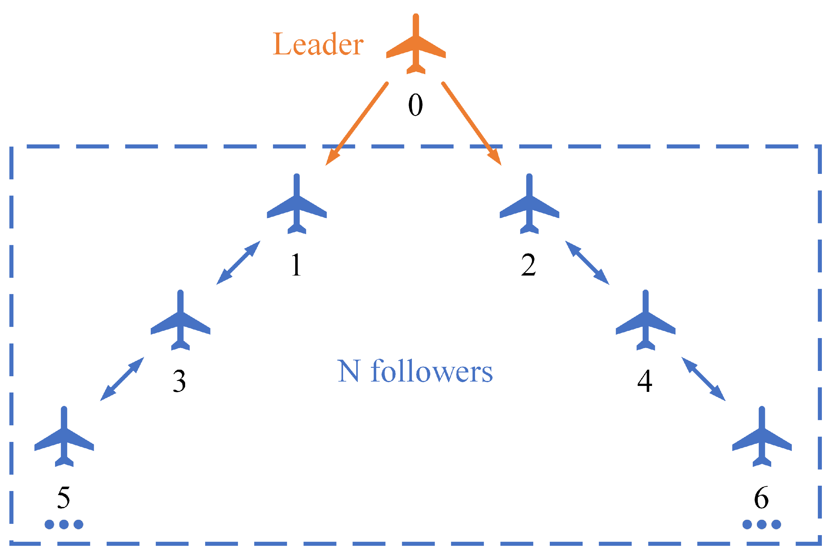
Figure 1.
The communication topology of the leader–follower multi-UAVs.
Figure 1.
The communication topology of the leader–follower multi-UAVs.
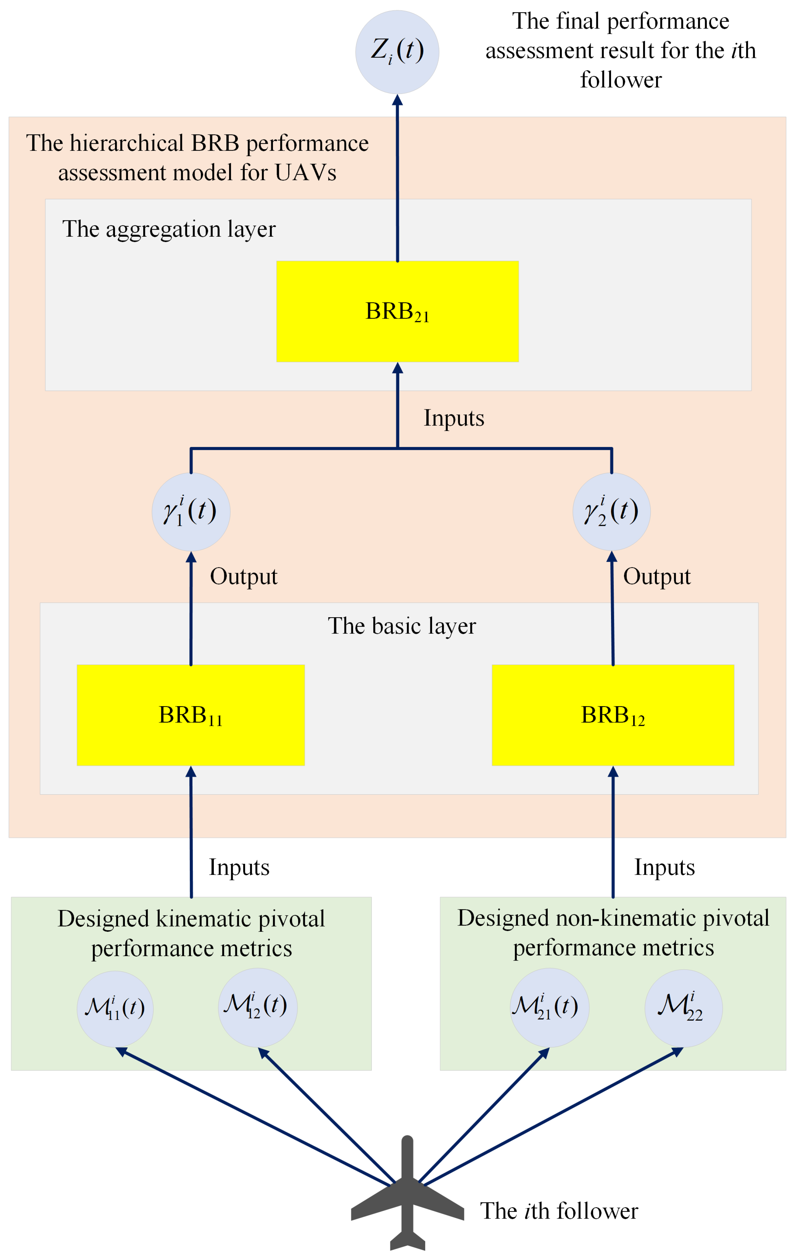
Figure 2.
The architecture of the hierarchical BRB performance assessment model for UAVs.
Figure 2.
The architecture of the hierarchical BRB performance assessment model for UAVs.
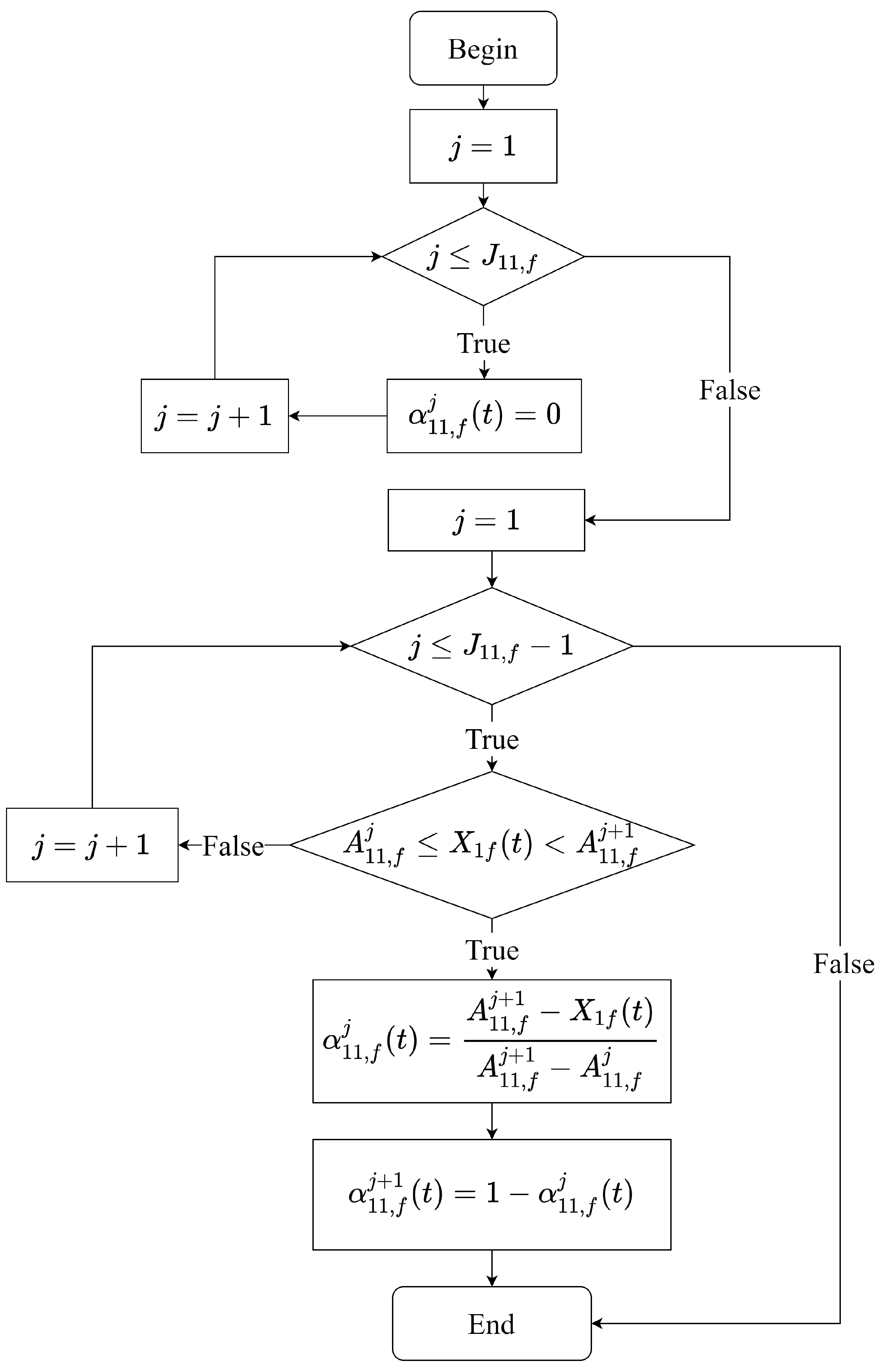
Figure 3.
Flowchart of calculating the belief degree of the jth referential value with respect to the fth antecedent attribute .
Figure 3.
Flowchart of calculating the belief degree of the jth referential value with respect to the fth antecedent attribute .
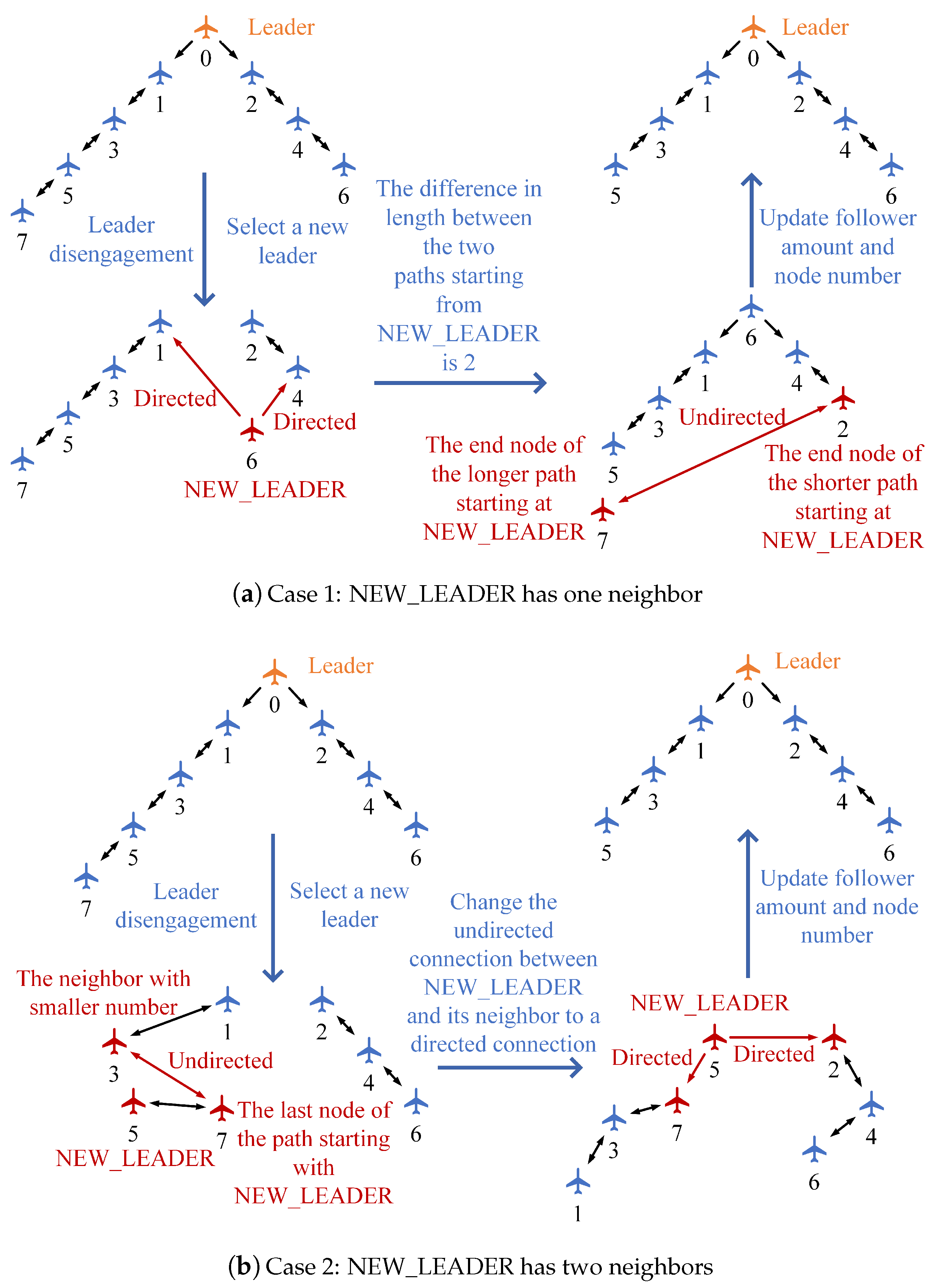
Figure 4.
The renewal of the swarm communication topology under leader disengagement.
Figure 4.
The renewal of the swarm communication topology under leader disengagement.
Figure 5.
The restoration of the swarm communication topology under follower disengagement.
Figure 5.
The restoration of the swarm communication topology under follower disengagement.
Figure 6.
The renewal of the swarm communication topology under new member addition.
Figure 6.
The renewal of the swarm communication topology under new member addition.
Figure 7.
The flight trajectories of the leader–follower multi-UAVs when .
Figure 7.
The flight trajectories of the leader–follower multi-UAVs when .
Figure 8.
The position trace error for each follower when .
Figure 8.
The position trace error for each follower when .
Figure 9.
The linear velocity for each follower when .
Figure 9.
The linear velocity for each follower when .
Figure 10.
The pitch angle for each follower when .
Figure 10.
The pitch angle for each follower when .
Figure 11.
The yaw angle for each follower when .
Figure 11.
The yaw angle for each follower when .
Figure 12.
The flight trajectories of the leader–follower multi-UAVs when .
Figure 12.
The flight trajectories of the leader–follower multi-UAVs when .
Figure 13.
The trajectory trace error for each follower when .
Figure 13.
The trajectory trace error for each follower when .
Figure 14.
The linear velocity for each follower when .
Figure 14.
The linear velocity for each follower when .
Figure 15.
The pitch angle for each follower when .
Figure 15.
The pitch angle for each follower when .
Figure 16.
The yaw angle for each follower when .
Figure 16.
The yaw angle for each follower when .
Figure 17.
Comparison of the performance scores for each follower.
Figure 17.
Comparison of the performance scores for each follower.
Figure 18.
The flight trajectories of the leader–follower multi-UAVs when .
Figure 18.
The flight trajectories of the leader–follower multi-UAVs when .
Figure 19.
The trajectory trace error for each follower when .
Figure 19.
The trajectory trace error for each follower when .
Figure 20.
The linear velocity for each follower when .
Figure 20.
The linear velocity for each follower when .
Figure 21.
The pitch angle for each follower when .
Figure 21.
The pitch angle for each follower when .
Figure 22.
The yaw angle for each follower when .
Figure 22.
The yaw angle for each follower when .
Figure 23.
The flight trajectories of the leader–follower multi-UAVs when .
Figure 23.
The flight trajectories of the leader–follower multi-UAVs when .
Figure 24.
The trajectory trace error for each follower when .
Figure 24.
The trajectory trace error for each follower when .
Figure 25.
The linear velocity for each follower when .
Figure 25.
The linear velocity for each follower when .
Figure 26.
The pitch angle for each follower when .
Figure 26.
The pitch angle for each follower when .
Figure 27.
The yaw angle for each follower when .
Figure 27.
The yaw angle for each follower when .
Figure 28.
The flight trajectories of the leader–follower multi-UAVs when .
Figure 28.
The flight trajectories of the leader–follower multi-UAVs when .
Table 1.
The innovation of the article compared with existing works.
Table 1.
The innovation of the article compared with existing works.
| Aspect | Existing Works | The Article |
|---|
| Reconfiguration | Geometry [9,16,36] | Communication |
| Swarm scale | Static [16,34,35] | Dynamic |
| Leader election | Single-source information [16] | Multi-sources information |
Table 2.
The referential information of the antecedent attribute of in the basic layer.
Table 2.
The referential information of the antecedent attribute of in the basic layer.
| Referential point | | | |
| Referential value | 28 | 33 | 38 |
Table 3.
The referential information of the antecedent attribute of in the basic layer.
Table 3.
The referential information of the antecedent attribute of in the basic layer.
| Referential point | | | |
| Referential value | 0 | 0.0005 | 0.001 |
Table 4.
The assessment grades of in the basic layer.
Table 4.
The assessment grades of in the basic layer.
| Referential point | | | | |
| Referential value | 20 | 40 | 60 | 80 |
Table 5.
The consequent belief distribution table of in the basic layer.
Table 5.
The consequent belief distribution table of in the basic layer.
| Rule Number | Antecedent Attributes | Consequent Belief Distribution |
|---|
| | {} |
|---|
| 1 | | | {0, 0.1, 0.1, 0.8} |
| 2 | | | {0, 0.2, 0.5, 0.3} |
| 3 | | | {0.2, 0.3, 0.3, 0.2} |
| 4 | | | {0, 0.2, 0.5, 0.3} |
| 5 | | | {0.1, 0.45, 0.45, 0} |
| 6 | | | {0.4, 0.4, 0.2, 0} |
| 7 | | | {0.2, 0.3, 0.3, 0.2} |
| 8 | | | {0.4, 0.4, 0.2, 0} |
| 9 | | | {0.6, 0.3, 0.1, 0} |
Table 6.
The referential information of the antecedent attribute of in the basic layer.
Table 6.
The referential information of the antecedent attribute of in the basic layer.
| Referential point | | | |
| Referential value | 500 | 1000 | 1500 |
Table 7.
The referential information of the antecedent attribute of in the basic layer.
Table 7.
The referential information of the antecedent attribute of in the basic layer.
| Referential point | | | |
| Referential value | 10 | 20 | 30 |
Table 8.
The assessment grades of in the basic layer.
Table 8.
The assessment grades of in the basic layer.
| Referential point | | | | |
| Referential value | 20 | 40 | 60 | 80 |
Table 9.
The consequent belief distribution table of in the basic layer.
Table 9.
The consequent belief distribution table of in the basic layer.
| Rule Number | Antecedent Attributes | Consequent Belief Distribution |
|---|
| | {} |
|---|
| 1 | | | {0.6, 0.3, 0.1, 0} |
| 2 | | | {0.4, 0.4, 0.2, 0} |
| 3 | | | {0.2, 0.3, 0.3, 0.2} |
| 4 | | | {0.4, 0.4, 0.2, 0} |
| 5 | | | {0.1, 0.45, 0.45, 0} |
| 6 | | | {0, 0.2, 0.5, 0.3} |
| 7 | | | {0.2, 0.3, 0.3, 0.2} |
| 8 | | | {0, 0.2, 0.5, 0.3} |
| 9 | | | {0, 0.1, 0.1, 0.8} |
Table 10.
The referential information of the antecedent attribute of in the aggregation layer.
Table 10.
The referential information of the antecedent attribute of in the aggregation layer.
| Referential point | | | |
| Referential value | 20 | 50 | 80 |
Table 11.
The referential information of the antecedent attribute of in the aggregation layer.
Table 11.
The referential information of the antecedent attribute of in the aggregation layer.
| Referential point | | | |
| Referential value | 20 | 50 | 80 |
Table 12.
The assessment grades of in the aggregation layer.
Table 12.
The assessment grades of in the aggregation layer.
| Referential point | | | | |
| Referential value | 20 | 40 | 60 | 80 |
Table 13.
The consequent belief distribution table of in the aggregation layer.
Table 13.
The consequent belief distribution table of in the aggregation layer.
| Rule Number | Antecedent Attributes | Consequent Belief Distribution |
|---|
| | {} |
|---|
| 1 | | | {0.6, 0.3, 0.1, 0} |
| 2 | | | {0.4, 0.4, 0.2, 0} |
| 3 | | | {0.2, 0.3, 0.3, 0.2} |
| 4 | | | {0.4, 0.4, 0.2, 0} |
| 5 | | | {0.1, 0.45, 0.45, 0} |
| 6 | | | {0, 0.2, 0.5, 0.3} |
| 7 | | | {0.2, 0.3, 0.3, 0.2} |
| 8 | | | {0, 0.2, 0.5, 0.3} |
| 9 | | | {0, 0.1, 0.1, 0.8} |
Table 14.
Correspondence between the identifier and the number in the swarm communication topology for each member of the multi-UAVs.
Table 14.
Correspondence between the identifier and the number in the swarm communication topology for each member of the multi-UAVs.
| Triggering Event | 0 | 1 | 2 | 3 | 4 | 5 |
|---|
| Initial correspondence | UAV 0 | UAV 1 | UAV 2 | UAV 3 | UAV 4 | UAV 5 |
| Addition of UAV 11 | UAV 0 | UAV 1 | UAV 2 | UAV 3 | UAV 4 | UAV 5 |
| Disengagement of UAV 0 | UAV 2 | UAV 1 | UAV 4 | UAV 3 | UAV 6 | UAV 5 |
| Disengagement of UAV 9 | UAV 2 | UAV 4 | UAV 1 | UAV 6 | UAV 3 | UAV 8 |
| Triggering Event | 6 | 7 | 8 | 9 | 10 | 11 |
| Initial correspondence | UAV 6 | UAV 7 | UAV 8 | UAV 9 | UAV 10 | |
| Addition of UAV 11 | UAV 6 | UAV 7 | UAV 8 | UAV 9 | UAV 10 | UAV 11 |
| Disengagement of UAV 0 | UAV 8 | UAV 7 | UAV 10 | UAV 9 | UAV 11 | |
| Disengagement of UAV 9 | UAV 5 | UAV 10 | UAV 7 | UAV 11 | | |
Table 15.
Connection retention rate (CRR) for the swarm communication topology using the proposed reconfiguration strategies.
Table 15.
Connection retention rate (CRR) for the swarm communication topology using the proposed reconfiguration strategies.
| Triggering Event | | | CRR |
|---|
| Addition of UAV 11 | 2 | 20 | 90% |
| Disengagement of UAV 0 | 6 | 18 | 67% |
| Disengagement of UAV 9 | 0 | 16 | 100% |


