Appointed-Time Leader-Following Consensus for Second-Order Multi-Agent Systems with Prescribed Performance Guarantees

Abstract

The appointed-time leader-following consensus problem for second-order multi-agent systems with external disturbance on directed graphs is addressed. A distributed controller based on the cumulative position difference and cumulative velocity difference is proposed, which does not require prior knowledge of external disturbances. It is shown that the proposed controller guarantees the prescribed performance of the controlled systems, namely, to keep the cumulative position difference within a predefined boundary envelope. Furthermore, by employing a novel performance function, it is ensured that the position tracking error converges to an arbitrarily small expected region within the appointed time. Different from most existing finite/fixed-time control methods, here the settling time and the convergence region can both be predefined, which are also independent of initial conditions and the system parameters. Finally, the theoretical results are verified by simulations.

1. Introduction

The cooperative control of multi-agent systems (MASs) has been widely investigated in many disciplines [1,2,3]. The leader-following consensus problem of MASs is an important problem for cooperative control that needs to be explored and solved [4,5,6,7,8]. In such MASs, the leader is a special agent whose movements are not affected by followers, and all the other followers are driven to follow the leader.

However, steady-state performance is mainly pursued in the leader-following consensus of MASs, while transient performance is less considered. To address this issue, the finite-time consensus protocol was developed [9], such that consensus in finite-time by using a distributed, event-triggered method is achieved, and in [10], an adaptive, dynamic sliding mode-based control protocol was proposed for heterogeneous MASs with uncertain dynamics and external disturbances to achieve finite-time consensus. Furthermore, so-called reset consensus protocols were proposed in [11,12], which provide faster convergence and less control effort than some conventional consensus controllers. In practice, it is usually expected that a large convergence rate and small overshoot can be guaranteed simultaneously, which is a trade-off. Sometimes, it is also desired that the controlled variable can be evolved within some certain boundary envelope. However, most of the literature, such as [9,10,11,12], cannot achieve this requirement. In order to achieve such expected performance requirements, the prescribed performance control (PPC) approach was firstly proposed in [13], solving the robust adaptive control problem for single systems. It is worth mentioning that guaranteeing the prescribed performance means that the controlled variable converges to a given region, achieving a large convergence rate with a small overshoot. Due to the capability of allowing people to prescribe the above-mentioned performance in practice, the concepts of PPC are widely used and applied in many single systems, such as strict feedback systems, non-strict-feedback systems and multi-degree-of-freedom robot systems, which can be found in [14,15,16,17,18,19]. Moreover, PPC has also been applied in MASs. In [20,21], PPC is applied to linear MASs with guaranteed prescribed performance to address the average consensus on undirected graphs. Subsequently, scholars began to study leader-following consensus in MASs under directed graphs to ensure prescribed performance [22,23,24,25,26]. Bechlioulis and Rovithakis designed a decentralized control law based on the Lyapunov theory to achieve leader-following consensus with guaranteed prescribed performance, for uncertain nonlinear MASs in [22]. PPC-based controllers were designed based on a backstepping method to address the consensus tracking problem for nonlinear MASs in [23,24,25,26]. Considering the agents’ state may be unmeasured, observers were designed to estimate state variables in [23,25,26]. However, applying the backstepping method may lead to the computational complexity explosion problem because of the repeated differentiation of virtual controllers at each step. In fact, we need a controller with lower complexity; in other words, we need the generation of control signals that only requires simple calculations.

When analyzing and dealing with consensus problems, in addition to ensuring that the control variable can be predefined with maximum allowable overshoot and minimum convergence rate, whether the consensus can be achieved in a finite-time is also an important issue. Because in some scenarios, such as military drone operations, it is necessary to ensure that the agents achieve formation consensus at the appointed time. Therefore, this topic has also attracted the attention and research of many scholars. The distributed finite-time consensus protocol was firstly proposed by Cortés [27]. Subsequently, various finite-time controllers for MASs have been designed in the current works [28,29,30]. However, in these studies, the convergence time depends on the initial states of agents, which means that if the initial states are not known a priori, and the convergence time for the consensus can not be estimated. To relax such a limitation, in [31,32], the fixed-time control was realized, and the upper bound of the settling time can be determined by some state-independent parameter by using the terminal sliding mode control technology. The cost is that the controller will be discontinuous, and in this case, it is difficult to be effectively applied in practical engineering. Therefore, it is necessary to find other control schemes, so that the controller is continuous, making it suitable for a wide range of practical engineering applications. In addition, most of the PPC methods in the literature usually use traditional exponential performance functions to quantitatively describe the transient and steady-state performance of the controlled systems, and sometimes it is difficult to guarantee that the controlled variable achieves the expected accuracy in fixed time.

Motivated by the above issues, we propose a PPC method to achieve leader-following consensus for the second-order MASs in this paper. The specified performance index is described as error constraints, and the constrained MAS is transformed into an unconstrained system by using the transformation error function. The controller of each agent only uses the position and velocity information of the neighbor agent and itself. The main contributions are given as follows.

• Compared with the works [28,29,30,33,34], where the consensus error accuracy cannot be specified a priori and the overshoot was neglected, the proposed controller based on PPC methods in this paper can guarantee the transient performance constraint, which means that the cumulative position difference evolves within a predefined region and the position tracking error can converge to a predefined arbitrarily small residual set within the appointed-time. The appointed time in the paper can be chosen arbitrarily.
• Compared with [22,23,24,25,26], we successfully drive the cumulative position difference to fall into the expected region in the appointed time by using a novel performance function. Furthermore, compared with the backstepping method in [23,24,25,26], our proposed scheme has low complexity.
• Compared with the work on sliding mode control-based fixed-time control [31,32], we only need to adjust several design parameters and the proposed controller is continuous, which it is more applicable for practical engineering.
• The control input of each agent is based on the position and velocity information of the neighbor agents, without the prior knowledge of the external disturbance of the dynamics of agents.

The rest of this paper is arranged as follows. In Section 2, the basic knowledge of graph theory, the core idea of PPC design, and the description of the problem studied in this paper are introduced. The main results are presented in Section 3, which includes the proposed controller and the proof of leader-following appointed-time consensus with prescribed performance. Simulation examples are presented in Section 4. Some conclusions are drawn in Section 5.

Notations: Throughout this paper, ${\mathbb{R}}^i$ denotes the i-dimensional Euclidean space; $\mid ·\mid$ is the absolute value of a real number; $\parallel ·\parallel$ is the Euclidean norm of a vector; ${\lambda }_{min}(·)$ and ${\lambda }_{max}(·)$, respectively, denote the smallest eigenvalue of a matrix and the largest eigenvalue of a matrix; matrix $K>0$ means K is positive definite. An M-matrix $\Lambda \in R^{n\times n}$ can be expressed in the form $\Lambda =sI-D$, where $D={(d_{ij})}_{n\times n}$ with $d_{ij}\ge 0$ for $\forall i,j$, and $s>\rho (D)$, with $\rho (D)$ being the spectral radius of matrix D.

2. Problem Formulation and Preliminaries

2.1. Graph Theory

The network among the N followers is represented by a directed graph $\mathcal{G}=\left\{\mathcal{V},\mathcal{E},\mathcal{A}\right\}$, where $\mathcal{V}=[{\vartheta }_1,{\vartheta }_2,\cdots ,{\vartheta }_N]$ is the set of nodes that represent the followers, with ${\vartheta }_i$ representing the ith follower, and $\mathcal{E}\subseteq \mathcal{V}\times \mathcal{V}$ is a directed edge set. $\mathcal{A}=(a_{ij})\in {\mathbb{R}}^{N\times N}$ is the adjacency matrix with $a_{ij}\in \left\{0,1\right\}$, $i,j=1,2,\cdots ,N$. In particular, if follower ${\vartheta }_i$ has access to follower ${\vartheta }_j$ information, then $a_{ij}=1$, which also means that edge $({\vartheta }_j,{\vartheta }_i)$ exists, otherwise $a_{ij}=0$, and in adjacency matrix $\mathcal{A}$, $a_{ii}=0$ for any i. For a directed graph, the Laplace matrix $L={[l_{ij}]}_{N\times N}$ related to the adjacency matrix is defined as $l_{ij}=-a_{ij}$ for $i\ne j$; $l_{ii}={\sum }_{j=1}^N{a}_{ij}.$ Matrix $B=\mathrm{diag}\left\{b_1,\cdots ,b_n\right\}$ with $b_i\in \left\{0,1\right\}$. In this paper, we only consider the case where there is only one leader. It is defined that when information flows from the leader to the follower ${\vartheta }_i$, $b_i=1$, otherwise, $b_i=0$. To distinguish the leader node from the follower nodes, we use ${\vartheta }_0$ to denote the leader and ${\vartheta }_1,{\vartheta }_2,\cdots ,{\vartheta }_N$ denotes the follower nodes. Then, the whole topology can be described by $\overline{\mathcal{G}}=\left\{\overline{\mathcal{V}},\overline{\mathcal{E}},\overline{\mathcal{A}}\right\}$ with $\overline{\mathcal{V}}=\mathcal{V}\cup \left\{{\vartheta }_0\right\}$.

A directed path is an ordered sequence of edges. For example, the edge sequence of a directed path from node ${\vartheta }_j$ to node ${\vartheta }_i$ has the form $({\vartheta }_j,{\vartheta }_k),({\vartheta }_k,{\vartheta }_m),\cdots ,({\vartheta }_n,{\vartheta }_i)$. In a directed graph, if every node except the root node (the root node has no parent node and has a directed path to other nodes) has a parent node, we call such a directed graph a spanning tree. If there is a (directed) spanning tree that is a subset of a graph, the graph is said to have (or contain) a (directed) spanning tree.

2.2. Prescribed Performance Control

In this section, we will introduce the main idea for the PPC approach, which is used for linearizable MIMO nonlinear systems [13].

First, the constraints are imposed on the controlled variable $e(t)$, which are designed as upper and lower bound constraints. The mathematical expression of the prescribed performance specification can be formulated by the following inequality [13]:

$$\left\{\begin{array}{c}-m\varsigma (t)<e(t)<\varsigma (t),ife(0)>0\hfill \\ -\varsigma (t)<e(t)<m\varsigma (t),ife(0)<0\hfill \end{array}\right.$$

(1)

for all $t\ge 0$, where $0\le m\le 1$ and $\varsigma (t)$ is the performance function satisfying that (i) $\varsigma (t)$ is a smooth function, (ii) $\varsigma (t)$ is positive and decreasing, and (iii) ${lim}_{t\to \infty }\varsigma (t)={\varsigma }_{\infty }$, where ${\varsigma }_{\infty }$ is a small positive constant.

Second, by means of spatial equivalent mapping, the nonlinear system under constraint (in the sense of (1)) can be transformed to the unconstrained system of $\epsilon$. More specifically, define

$$\varrho (t)=\Gamma (\epsilon )$$

(2)

where $\varrho (t)=\frac{e(t)}{\varsigma (t)}$, $\epsilon$ is the transformed error, and $\Gamma$ satisfies

(i)

$\Gamma (\epsilon )$ is strictly increasing and smooth

(ii)

$\left\{\begin{array}{c}-m<\Gamma (\epsilon )<1,ife(0)>0\hfill \\ -1<\Gamma (\epsilon )<m,ife(0)<0\hfill \end{array}\right.$

(iii)

if $e(0)>0$$\left\{\begin{array}{c}{lim}_{\epsilon \to -\infty }\Gamma (\epsilon )=-m\hfill \\ {lim}_{\epsilon \to +\infty }\Gamma (\epsilon )=1\hfill \end{array}\right.$

if $e(0)<0$$\left\{\begin{array}{c}{lim}_{\epsilon \to -\infty }\Gamma (\epsilon )=-1\hfill \\ {lim}_{\epsilon \to +\infty }\Gamma (\epsilon )=m\hfill \end{array}\right.$

A diagrammatic sketch of $\epsilon (t)$ is represented in Figure 1. The boundedness of $\epsilon$ leads to $-m<\varrho (t)<1$ in the case of $e(0)\ge 0$ and $-1<\varrho (t)<m$ in the case of $e(0)<0$. Hence, the evolution of $e(t)$ with some constraint specification, namely, (1) holds if $\epsilon$ is bounded.

2.3. Problem Statement

We consider the MASs with N followers and a leader over directed graphs. The double-integrator dynamics of follower i are described as follows:

$$\left\{\begin{array}{c}{\dot{x}}_i(t)=v_i(t)\hfill \\ {\dot{v}}_i(t)=u_i(t)+d_i(t)\hfill \end{array}\right.$$

(3)

where $x_i(t),v_i(t),u_i(t),d_i(t)\in \mathbb{R}$ are the position, velocity, control input, and external disturbance of the ith follower, respectively, for $i=1,\cdots ,N$. Let $x={[x_1,x_2,\cdots ,x_N]}^T$ and $v={[v_1,v_2,\cdots ,v_N]}^T$ be the stack vector of MASs. The leader’s dynamics is described as

$${\dot{x}}_0(t)=v_0(t)$$

(4)

where $x_0\in \mathbb{R}$ is leader’s position and $v_0\in \mathbb{R}$ is leader’s velocity. In order to simplify the subsequent controller design of each follower, the following assumptions are required.

Assumption 1.

The graph $\overline{\mathcal{G}}$ contains a spanning tree with the root node being the leader, and there exists no self-loop for each vertex.

Assumption 2.

$v_0(t)$ is piecewise continuous and ${\dot{v}}_0$ is bounded.

Assumption 3.

For the external disturbance $d_i(t)$, there exists a positive constant $\overline{d}$ such that $|d_i|\le \overline{d}$.

We use $e_{ix}$ and $e_{iv}$ to represent the cumulative position difference and the cumulative velocity difference of the ith follower agent, respectively, which are defined as follows:

$$e_{ix}=\sum _{j=1}^N{a}_{ij}(x_i-x_j)+b_i(x_i-x_0)$$

(5)

$$e_{iv}=\sum _{j=1}^N{a}_{ij}(v_i-v_j)+b_i(v_i-v_0).$$

(6)

Then, we define the position tracking error ${\delta }_{ix}$ and the velocity tracking error ${\delta }_{iv}$ for the ith follower as ${\delta }_{ix}=x_i-x_0$, ${\delta }_{iv}=v_i-v_0$.

Definition 1

([35]). (Practical appointed-time consensus for leader-following networks): For the leader-follower networks described by MASs (3) and (4), the practical appointed-time consensus can be achieved if the following conditions hold:

$$\mid {\delta }_{ix}(t)\mid \le k_x,\forall t\ge t_f$$

and

$$\mid {\delta }_{iv}(t)\mid \le k_v,\forall t\ge t_f$$

where $t_f$ is the appointed setting time, $k_x>0$ is the maximum allowable steady-state error, and $k_v>0$.

Our goal is to design a distributed consensus control protocol for linear MASs expressed by (3) and (4) such that the following apply:

(1) The practical appointed-time consensus as defined by Definition 1 is achieved.

(2) The cumulative position difference $e_{ix}$ evolves within a prescribed region, which is quantified as

$$-{\varsigma }_i(t)<e_{ix}(t)<{\varsigma }_i(t),i=1,\cdots ,N$$

(7)

where ${\varsigma }_i(t)>0$ is the performance function.

(3) The control input $u_i$ and the velocity of the ith follower, i.e., $v_i$, are bounded.

Before moving on, three lemmas are introduced as follows, which will be employed in the proof of the main results.

Lemma 1

([36]). Let $H\in R^{N\times N}$ be a nonsingular M-matrix, then there exists a diagonal positive definite matrix $Q={(\mathrm{diag}(q))}^{-1}$ such that $QH+H^{T}Q$ is positive definite, where $q=H^{-1}\mathbf{1}$ and $\mathbf{1}={[1,\cdots ,1]}^T\in {\mathbb{R}}^N$.

Lemma 2

(H$\ddot{o}$lder’s Inequality [37]). For $p_i\in R$ and $q_i\in R$, the following inequality is satisfied:

$$\sum _{i=1}^n|p_i{q}_i|\le \{\sum _{i=1}^n|p_i{|}^a{\}}^{1/a}\{\sum _{i=1}^n|q_i{{|}^b\}}^{1/b}$$

with $a>1$ and $b>1$ being real numbers and $1/a+1/b=1$.

Lemma 3

([38]). Consider a class of differential equation such that $\dot{\chi }=\beta (t,\chi (t))$, $\chi (0)={\chi }^0\in {\Pi }_{\chi }$ with β: ${\mathbb{R}}_{+}\times {\Pi }_{\chi }\to {\mathbb{R}}^N$ and ${\Pi }_{\chi }\subset {\mathbb{R}}^N$ being a non-empty open set. If the conditions hold:

(i) 

β is locally Lipschitz over χ;

(ii) 

β is continuous over t;

(iii) 

β is locally integrable over t, $\forall \chi (t)\in {\Pi }_{\chi }$.

A unique maximal solution can be obtained that χ: [0,$t_{max}$) $\to {\Pi }_{\chi }$ of $\dot{\chi }(t)=\beta (t,\chi (t))$ on the time domain $[0,t_{max})$ with $t_{max}\in \left\{{\mathbb{R}}_{+},\infty \right\}$, and consequently, $\chi (t)\in {\Pi }_{\chi }$, $t\in [0,t_{max})$. Furthermore, if $t_{max}<\infty$ and ${\Pi }_{\chi }^{*}\subset {\Pi }_{\chi }$, there exists a time moment $t^{*}\in [0,t_{max})$ such that $\chi (t^{*})\notin {\Pi }_{\chi }^{*}$.

3. Main Results

Define $e_x={[e_{1x},\cdots ,e_{Nx}]}^T$, $e_v={[e_{1v},\cdots ,e_{Nv}]}^T$. The dynamic model of the cumulative difference in vector form is written as follows:

$$\left\{\begin{array}{c}{\dot{e}}_x=e_v\hfill \\ {\dot{e}}_v=(L+B)(u+d-\mathbf{l}{\dot{v}}_0)\hfill \end{array}\right.$$

(8)

where $d={[d_1,\cdots ,d_N]}^T$ and $\mathbf{1}={[1,\cdots ,1]}^T\in {\mathbb{R}}^N$.

Let us define the normalized error ${\xi }_i$ as ${\xi }_i=\frac{e_{ix}}{{\varsigma }_i},i=1,\cdots ,N$. Then, let

$$\xi ={[{\xi }_1,\cdots ,{\xi }_N]}^T={[\frac{e_{1x}}{{\varsigma }_1},\cdots ,\frac{e_{Nx}}{{\varsigma }_N}]}^T=C(t)e_x$$

(9)

where $C(t)=\mathrm{diag}(\frac{1}{{\varsigma }_1(t)},\cdots ,\frac{1}{{\varsigma }_N(t)})$, with ${\varsigma }_i(t),i=1,\cdots ,N$ being performance functions to be determined later.

Define the transformation error

$${\epsilon }_i=ln(\frac{1+{\xi }_i}{1-{\xi }_i}),i=1,\cdots ,N.$$

(10)

Let $\epsilon ={[{\epsilon }_1,\cdots ,{\epsilon }_N]}^T.$ Differentiating $\epsilon$ with respect to t obtains

$$\dot{\epsilon }=\mathsf{\Phi }(t)(e_v-\dot{S}(t)\xi )$$

(11)

where $\mathsf{\Phi }(t)=\mathrm{diag}(\frac{2}{(1-{\xi }_1^2){\varsigma }_1},\cdots ,\frac{2}{(1-{\xi }_N^2){\varsigma }_N})$, $S(t)=\mathrm{diag}({\varsigma }_1(t),\cdots ,{\varsigma }_N(t))$. In order to simplify the description of $\mathsf{\Phi }(t)$ and $S(t)$, $\mathsf{\Phi }$ and S are used to denote $\mathsf{\Phi }(t)$ and $S(t)$, respectively, in the following content.

Next, partly inspired by [39], a novel smooth performance function is defined as

$${\varsigma }_i(t)=\left\{\begin{array}{cc}({\varsigma }_i(0)-\frac{t}{t_f})e^{(1-\frac{t_f}{t_f-t})}+{\varsigma }_i(t_f),\hfill & t\in [0,t_f)\hfill \\ {\varsigma }_i(t_f),\hfill & t\in [t_f,+\infty )\hfill \end{array}\right.$$

(12)

where $i=1,\cdots ,N$, ${\varsigma }_i(0)>\frac{5}{4}$, and ${\varsigma }_i(t_f)>0$.

With the given performance function (12), Lemma 4 is introduced.

Lemma 4.

The performance function (12) satisfies the following properties:

(1) 

${\varsigma }_i(t)>0$

(2) 

${\dot{\varsigma }}_i(t)\le 0$

(3) 

${lim}_{t\to t_f}{\varsigma }_i(t)={\varsigma }_i(t_f)$ and ${\varsigma }_i(t)={\varsigma }_i(t_f)$ for any $t\ge t_f$ where ${\varsigma }_i(t_f)$ represents any small constant and $t_f$ is the setting time.

(4) 

${\varsigma }_i(t)$ is a smooth function.

The proof of Lemma 4 can be found in Appendix A.

Remark 1.

In the present research results on PPC, a conventional performance function [13] is shown in (13). Compared with ${\overline{\varsigma }}_i(t)$, our proposed performance function in (12) has the property that it guarantees appointed-time convergence, which does not hold for ${\overline{\varsigma }}_i(t)$ due to ${lim}_{t\to \infty }{\overline{\varsigma }}_i(t)={\overline{\varsigma }}_i(\infty )$

$${\overline{\varsigma }}_i(t)=({\overline{\varsigma }}_i(0)-{\overline{\varsigma }}_i(\infty ))e^{-l_{i}t}+{\overline{\varsigma }}_i(\infty )$$

(13)

where ${\overline{\varsigma }}_i(\infty )>0$, ${\overline{\varsigma }}_i(0)>0$ and $l_i>0$.

The distributed control protocol is given as follows:

$$u_i=-k_1{\epsilon }_i(t)-k_2{e}_{iv}(t),{\vartheta }_i\in \mathcal{V}$$

(14)

with $k_1$, $k_2$ being positive constants, and $e_{iv}(t)$, ${\epsilon }_i(t)$ have been defined in (6) and (10), respectively.

With control input (14), system (8) can be rewritten as follows:

$$\left\{\begin{array}{c}{\dot{e}}_x=e_v\hfill \\ {\dot{e}}_v=(L+B)(-k_1\epsilon (t)-k_2{e}_v(t)+d(t)-\mathbf{l}{\dot{v}}_0).\hfill \end{array}\right.$$

(15)

The following theorem presents our main results.

Theorem 1.

Under Assumptions 1 and 2, consider MASs (3) and (4) with a directed graph. With the control protocol given by (14), if the controller parameters are chosen such that $k_1>\sqrt{\frac{2+|\overline{\varphi }{|}^2}{w{\lambda }_1}}$, $k_1^2\beta <\frac{{\lambda }_{min}^2(L+B)}{w^2{\parallel P(L+B)\parallel }^2}$, and $\frac{{\lambda }_{min}(L+B)-\sqrt{\alpha }}{w^2{k}_1^2{\parallel P(L+B)\parallel }^2}<k_2<\frac{{\lambda }_{min}(L+B)+\sqrt{\alpha }}{w^2{k}_1^2{\parallel P(L+B)\parallel }^2}$ with $0<\omega <\frac{1}{k_1{\lambda }_{max}(P)}$, $P={(\mathrm{diag}({(L+B)}^{-1}\mathbf{1}))}^{-1}$, $\parallel \mathsf{\Phi }\parallel \le \overline{\varphi }$, $\alpha ={\lambda }_{min}^2(L+B)-w^2{k}_1^2\beta {\parallel P(L+B)\parallel }^2$, $\beta =1+2w{k}_1\parallel \overline{\varphi }P\parallel +{\lambda }_{max}^2(L+B)k_1^2$, ${\lambda }_1={\lambda }_{min}(P(L+B)+{(L+B)}^{T}B)$ and let ${\varsigma }_i(0)>max\left\{|e_{ix}(0)|,\frac{5}{4}\right\}$, then the control objectives mentioned in Section 2.3 can be achieved.

Proof. 

It follows from Assumption 1 that $L+B$ is a nonsingular M-matrix [40]. According to Lemma 1, there exists a diagonally positive definite matrix $P={(\mathrm{diag}(q))}^{-1}$, with $q={(L+B)}^{-1}\mathbf{1}$ and $\mathbf{1}={[1,\cdots ,1]}^T\in {\mathbb{R}}^N$. We propose the following Lyapunov function candidate:

$$V(\epsilon ,e_v)=\frac{1}{2}{\epsilon }^T\epsilon +\frac{1}{2}{e_v}^T{e}_v+\omega {\epsilon }^T{k}_{1}P{e}_v$$

(16)

with $0<\omega <\frac{1}{k_1{\lambda }_{max}(P)}$ and $k_1>0$. It can be verified that

$$V=[{\epsilon }^T,e_v^T]\left[\begin{array}{cc}\frac{I}{2}& \frac{w}{2}{k}_{1}P\\ \frac{w}{2}{k}_{1}P& \frac{I}{2}\end{array}\right][\begin{array}{c}\epsilon \\ e_v\end{array}]>0,$$

which means that the Lyapunov function is positive definite. Differentiating (16) with respect to t obtains

$$\begin{array}{cc}\hfill \dot{V}& ={\epsilon }^T[\mathsf{\Phi }(e_v-\dot{S}\xi )]\hfill \\ \hfill & +\omega {\epsilon }^T{k}_{1}P(L+B)(-k_1\epsilon -k_2{e}_v+d-\mathbf{1}{\dot{v}}_0)\hfill \\ \hfill & +{\omega e_v}^T{k}_{1}P[\mathsf{\Phi }(e_v-\dot{S}\xi )]\hfill \\ & +{e_v}^T(L+B)(-k_1\epsilon -k_2{e}_v+d-\mathbf{1}{\dot{v}}_0)\hfill \end{array}$$

Differentiating $\xi$ versus time obtains

$$\dot{\xi }=C(t)(e_v-\dot{S}\xi )$$

(17)

Define the open set

$${\mathsf{\Omega }}_{\xi }=\underset{Ntimes}{\underbrace{(-1,1)\times \cdots \times (-1,1)}}$$

(18)

Since the performance functions ${\varsigma }_i(t),i=1,\cdots ,N$ are selected such that ${\varsigma }_i(0)>max\left\{|e_{ix}(0)|,\frac{5}{4}\right\},i=1,\cdots ,N$, then $|{\xi }_i(0)|<1,i=1,\cdots ,N$ is satisfied. Suppose there is a time instant ${\tau }_{max}$ after which $\xi (t)$ escapes from ${\mathsf{\Omega }}_{\xi }$. It is deduced

$$\xi (t)\in {\mathsf{\Omega }}_{\xi },\forall t\in [0,{\tau }_{max})$$

Then, it is easy to find that there exists $t_{s_1}\in [0,{\tau }_{max})$ and $t_{s_2}\in [0,{\tau }_{max})$, such that the following inequalities hold,

$${\varsigma }_i(t)-e_{ix}(t)>\frac{\mu {\varsigma }_i(t_f)}{e^{\parallel s(0)\parallel }+1},t\in [0,t_{s_1})$$

(19)

$${\varsigma }_i(t)+e_{ix}(t)>\mu \frac{e^{-\parallel s(0)\parallel }{\varsigma }_i(t_f)}{e^{-\parallel s(0)\parallel }+1},t\in [0,t_{s_2})$$

(20)

where $s(0)=[\parallel \epsilon (0)\parallel ,\parallel e_v(0){\parallel ]}^T$, $\mu$ is a constant to be determined. Define $t_s=min\left\{t_{s_1},t_{s_2}\right\}$.

Define ${\mathsf{\Omega }}_{\xi }^{*}={[R_1,R_2]}^N$ with $R_1=-1+\frac{\mu e^{-\parallel s(0)\parallel }{\varsigma }_i(t_f)}{(e^{-\parallel s(0)\parallel }+1){\varsigma }_i(t)}$ and $R_2=1-\frac{\mu {\varsigma }_i(t_f)}{(e^{\parallel s(0)\parallel }+1){\varsigma }_i(t)}$. ${\mathsf{\Omega }}_{\xi }^{*}$ is the subset of ${\mathsf{\Omega }}_{\xi }$, and $\xi (t)$ escapes from ${{\mathsf{\Omega }}_{\xi }}^{*}$ only when $t\ge t_s$. In other words,

$$\xi (t)\in {\mathsf{\Omega }}_{\xi }^{*}\subset {\mathsf{\Omega }}_{\xi },\forall t\in [0,t_s)$$

(21)

Owing to (21) and the boundedness of ${\varsigma }_i(t)$ by its construction, it can be obtained that there exists a $\overline{\varphi }>0$, such that $\parallel \mathsf{\Phi }\parallel \le \overline{\varphi }$, for all $t\in [0,t_s)$. Then the following inequality is satisfied for all $t\in [0,t_s)$.

$$\begin{array}{cc}\hfill \dot{V}& \le \frac{1}{2}{(\parallel \epsilon \parallel }^2|\overline{\varphi }{|}^2+\parallel e_v{\parallel }^2)+\parallel \overline{\varphi }\dot{S}\xi \parallel \parallel \epsilon \parallel -\frac{\omega }{2}{k}_1^2{\lambda }_1{\parallel \epsilon \parallel }^2+\frac{1}{2}{\parallel \epsilon \parallel }^2+\omega \parallel \overline{\varphi }{k}_{1}P\parallel \parallel e_v{\parallel }^2\hfill \\ & +\omega \parallel {\xi }^T\dot{S}\overline{\varphi }{k}_{1}P\parallel \parallel e_v\parallel -k_2{\lambda }_{min}(L+B)\parallel e_v{\parallel }^2+\frac{1}{2}{\lambda }_2\parallel e_v{\parallel }^2+\frac{1}{2}{\parallel \epsilon \parallel }^2+\omega \parallel k_{1}P(L+B)\mathbf{1}{\dot{v}}_0\parallel \parallel \epsilon \parallel \hfill \\ & +\parallel (L+B)\mathbf{1}{\dot{v}}_0\parallel \parallel e_v\parallel +\frac{{\omega }^2}{2}\parallel k_1{F\parallel }^2\parallel e_v{\parallel }^2+\omega \parallel k_{1}P(L+B)\parallel \sqrt{N}\overline{d}\parallel {\epsilon }^T\parallel +\parallel (L+B)\parallel \sqrt{N}\overline{d}\parallel e_v^T\parallel \hfill \end{array}$$

where ${\lambda }_1={\lambda }_{min}(P(L+B)+{(L+B)}^{T}P)$, $F=P(L+B)k_2$, ${\lambda }_2=k_1^2{{\lambda }^2}_{max}(L+B)$. It is noted that in the above expression, ${\epsilon }^T\mathsf{\Phi }{e}_v\le \frac{1}{2}{(\parallel \epsilon \parallel }^2|\overline{\varphi }{|}^2+\parallel e_v{\parallel }^2)$ is obtained by using $x^{T}y\le \frac{1}{2}{(\parallel x\parallel }^2+{\parallel y\parallel }^2)$, and $-{e_v}^T(L+B)\mathbf{1}{\dot{v}}_0\le \parallel (L+B)\mathbf{1}{\dot{v}}_0\parallel \parallel e_v\parallel$ is obtained by using ${\sum }_{i=1}^N|x_i{y}_i|\le {({\sum }_{i=1}^N|x_i{|}^2)}^{\frac{1}{2}}{({\sum }_{i=1}^N|y_i{|}^2)}^{\frac{1}{2}}$.

Moreover, one yields

$$\begin{array}{cc}\hfill \dot{V}& \le -s^{T}Ws+b^{T}s\hfill \\ \hfill & \le -{\lambda }_{min}{(W)\parallel s\parallel }^2+\parallel b\parallel \parallel s\parallel \hfill \end{array}$$

(22)

where $s=[\parallel \epsilon \parallel ,\parallel e_v{\parallel ]}^T$, $W=\mathrm{diag}(w_1,w_2)$, $w_1=\frac{\omega }{2}{k}_1^2{\lambda }_1-1-\frac{1}{2}{|\overline{\varphi }|}^2$, $w_2=k_2{\lambda }_{min}(L+B)-\frac{1}{2}-\omega \parallel k_1\overline{\varphi }P\parallel -\frac{{\omega }^2}{2}{\parallel k_{1}F\parallel }^2-\frac{1}{2}{\lambda }_2$ and $b={[b_1,b_2]}^T$ with $b_1=\parallel \overline{\varphi }\dot{S}\xi \parallel +\omega \parallel k_{1}P(L+B)\mathbf{1}{\dot{v}}_0\parallel +\omega \parallel k_{1}P(L+B)\parallel \sqrt{N}\overline{d}$, $b_2=\omega \parallel {\xi }^T\dot{S}\overline{\varphi }{k}_{1}P\parallel +\parallel (L+B)\mathbf{1}{\dot{v}}_0\parallel +\parallel (L+B)\parallel \sqrt{N}\overline{d}$.

By choosing appropriate $k_1$ and $k_2$, we can ensure that W is positive definite. More specifically, by chosing $k_1>\sqrt{\frac{2+|\overline{\varphi }{|}^2}{w{\lambda }_1}}$, it can be verified that $w_1>0$. To guarantee that $w_2>0$, one obtains the following inequality

$$w^2{k}_1^2{\parallel P(L+B)\parallel }^2{k}_2^2-2{\lambda }_{min}(L+B)k_2+\beta <0$$

(23)

where $\beta =1+2w{k}_1\parallel \overline{\varphi }P\parallel +k_1^2{\lambda }_{max}^2(L+B)$. We further require that $\alpha ={\lambda }_{min}^2(L+B)-w^2{k}_1^2\beta {\parallel P(L+B)\parallel }^2>0$, which is equivalent to $k_1^2\beta <\frac{{\lambda }_{min}^2(L+B)}{w^2{\parallel P(L+B)\parallel }^2}$, and in this case, $\frac{{\lambda }_{min}(L+B)-\sqrt{\alpha }}{w^2{k}_1^2{\parallel P(L+B)\parallel }^2}<k_2<\frac{{\lambda }_{min}(L+B)+\sqrt{\alpha }}{w^2{k}_1^2{\parallel P(L+B)\parallel }^2}$.

Then it follows from (22) that $\dot{V}<0$ if $\parallel s\parallel >\frac{\parallel b\parallel }{{\lambda }_{min}(W)}$. Owing to Assumption 2, we obtain that $\parallel b\parallel$ is finite. It is concluded that

$$\parallel s\parallel \le s^{*}=max\left\{\parallel s(0)\parallel ,\frac{\parallel b\parallel }{{\lambda }_{min}(W)}\right\},\forall t\in [0,t_s)$$

(24)

From (24), it can be further obtained that $\parallel e_v(t)\parallel \le \parallel s(t)\parallel \le s^{*}$, and $\parallel \epsilon (t)\parallel \le s^{*}$ for all $t\in [0,t_s)$. Through (10), (19), and (20), it is obtained that for $\forall t\in [0,t_s)$

$$-1<R_1<{\sigma }_1\le {\xi }_i(t)\le {\sigma }_2<R_2<1$$

(25)

where ${\sigma }_1=\frac{e^{-s^{*}}-1}{e^{-s^{*}}+1}$ and ${\sigma }_2=\frac{e^{s^{*}}-1}{e^{s^{*}}+1}$. It is noted that if $\parallel s(0)\parallel >\frac{\parallel b\parallel }{{\lambda }_{min}(W)}$, $R_1<{\sigma }_1$ and ${\sigma }_2<R_2$ can be guaranteed by selecting $\mu \in (0,2)$. Similarly, if $\frac{\parallel b\parallel }{{\lambda }_{min}(W)}>\parallel s(0)\parallel$, $\mu$ can be chosen such that $\mu \le 2(e^{\parallel s(0)\parallel }+1)/(e^{\frac{\parallel b\parallel }{{\lambda }_{min}(W)}}+1)$.

Define ${\mathsf{\Omega }}_{\xi }^{**}={[{\sigma }_1,{\sigma }_2]}^N$. From (25) we can obtain that at all $t\in [0,t_s)$, $\xi (t)\in {\mathsf{\Omega }}_{\xi }^{**}\subset {\mathsf{\Omega }}_{\xi }^{*}\subset {\mathsf{\Omega }}_{\xi }$. Hence, assuming $t_s<\infty$, it follows from Lemma 3 that ${\mathsf{\Omega }}_{\xi }^{**}\subset {\mathsf{\Omega }}_{\xi }^{*}$ implies the existence of $t^{\prime }\in [0,t_s)$, such that $\xi (t^{\prime })\notin {\mathsf{\Omega }}_{\xi }^{**}$, which contradicts (25). Therefore, $t_s$ and then ${\tau }_{max}$ can be extended to $+\infty$. Thus we can obtain, for any time $-{\varsigma }_i(t)<e_{ix}<{\varsigma }_i(t)$. Moreover, owing to Lemma 4, it is easy to verify that $\underset{t\ge t_f}{lim}|e_{ix}(t)|<{\varsigma }_i(t_f),i=1,\cdots ,N$.

In addition, according to [22], one has

$$\parallel {\delta }_m\parallel \le k_N\parallel e_m\parallel ,m\in \left\{x,v\right\}$$

(26)

where ${\delta }_x={[{\delta }_{1x},\cdots ,{\delta }_{Nx}]}^T$, ${\delta }_v={[{\delta }_{1v},\cdots ,{\delta }_{Nv}]}^T$, and $k_N=\frac{N^2+N-1}{{(\frac{N-1}{N})}^{\frac{N-1}{2}}}$.

Therefore, it can be further obtained that

$$\underset{t\ge t_f}{lim}|{\delta }_{ix}|<k_N\sqrt{N}\underset{1\le i\le N}{max}({\varsigma }_i(t_f))$$

(27)

$$|{\delta }_{iv}|\le k_N\parallel e_v\parallel \le k_N{s}^{*},i=1,\cdots ,N$$

(28)

From (28), we can verify that $e_{iv}$ and $v_i$ are also bounded.

Moreover, the control input $u_i$ remains bounded:

$$|u_i|\le (k_1+k_2)s^{*},i=1,\cdots ,N$$

(29)

This completes the proof of the Theorem 1. □

Remark 2.

It is noted that in [35], the control input information of its neighbor followers is needed to achieve appointed-time consensus for second-order MASs with guaranteed prescribed performance. As a contrast, our proposed controller of the ith follower does not need the control input information of its neighbors.

In order to summarize the main results, we provide the following algorithm in

Table 1. Distributed consensus control algorithm of second-order MASs.

Algorithm 1	Distributed consensus control algorithm of second-Order MASs
step 1	obtain the position $x_0(t)$ and velocity $v_0(t)$ of leader
step 2	select the $t_f$, ${\varsigma }_i(0)$, ${\varsigma }_i(t_f)$ for $i=1,\cdots ,7$
step 3	select the suitable control gain $k_1$, $k_2$ in (14) according to Theorem 1.

, and the consensus control block diagram is shown in Figure 2.

4. Simulations

This section presents an example to validate the effectiveness of our proposed control protocol. Consider the MASs with one leader agent and seven following agents in this example, wherein the dynamics of the leader and the followers are represented by (3) and (4), respectively. Figure 3 shows the information flow among all agents, with which Assumption 1 is satisfied. From Figure 3, the Laplace matrix L, the adjacency matrix $\mathcal{A}$, and matrix B are given as

$$L=\left[\begin{array}{ccccccc}0& 0& 0& 0& 0& 0& 0\\ -1& 1& 0& 0& 0& 0& 0\\ 0& -1& 1& 0& 0& 0& 0\\ 0& 0& -1& 1& 0& 0& 0\\ 0& 0& 0& -1& 1& 0& 0\\ -1& 0& 0& 0& -1& 2& 0\\ 0& 0& 0& 0& 0& -1& 1\end{array}\right]$$

$$\mathcal{A}=\left[\begin{array}{ccccccc}0& 0& 0& 0& 0& 0& 0\\ 1& 0& 0& 0& 0& 0& 0\\ 0& 1& 0& 0& 0& 0& 0\\ 0& 0& 1& 0& 0& 0& 0\\ 0& 0& 0& 1& 0& 0& 0\\ 1& 0& 0& 0& 1& 0& 0\\ 0& 0& 0& 0& 0& 1& 0\end{array}\right]$$

$B=diag\left\{1,0,0,0,0,0,1\right\}$. Let $p_i={[x_i,y_i]}^T$, $v_i={[v_{x_i},v_{y_i}]}^T,i\in \left\{1,\cdots ,7\right\}$, be the position and the velocity of each follower i, respectively. The initial values of the followers are set as $p_1(0)={[0.2,-1]}^T$, $p_2(0)={[-1,1]}^T$, $p_3(0)={[1,0]}^T$, $p_4(0)={[1,1]}^T$, $p_5(0)={[-1,-0.5]}^T$, $p_6(0)={[1,-1]}^T$, $p_7(0)={[-1,1]}^T$, $v_1(0)={[1,1]}^T$, $v_2(0)={[-0.5,0.5]}^T$, $v_3(0)={[1,-1]}^T$, $v_4(0)={[1.5,1]}^T$, $v_5(0)={[0,0]}^T$, $v_6(0)={[-1,-1]}^T$, $v_7(0)={[0.5,1]}^T$. The vector of disturbance for followers on x-dimension and y-dimension are both set as $d(t)=0.1\times {[cos(0.6t),sin(0.6t),sin(0.6t),sin(0.6t),sin(0.6t),sin(0.6t),sin(0.6t)]}^T$.

Let $p_0={[x_0,y_0]}^T$, $v_0={[sin(t),sin(t)]}^T$ be the position and the velocity of the leader. The values of the leader’s initial position and initial velocity are set as $p_0(0)={[0,0]}^T$ and $v_0(0)={[0,0]}^T$, respectively.

The designed parameters in (12) are selected as $t_f=6 \mathrm{s}$, ${\varsigma }_i(0)=3.2$, ${\varsigma }_i(t_f)=0.0095$$(i=1,\cdots ,7)$. Finally, by using Theorem 1, the control parameters are selected as $k_1=64$, $k_2=150$. In order to prove that the controller proposed in this paper achieves the appointed-time leader–follower consensus for the MASs with the prescribed performance, the simulation results will be compared with the existing controller without PPC [6], whose controller is given as follows:

$$u_i(t)=-k_1(\sum _{j=1}^N{a}_{ij}(x_i-x_j)-b_i(x_i-x_0))-k_2(\sum _{j=1}^N{a}_{ij}(v_i-v_j)-b_i(v_i-v_0))$$

(30)

where $k_1=64$ and $k_2=150$, and Wei’s controller in [35], whose controller is given as follows:

$$u_i\left(t\right)={\left(l_{ii}+b_i\right)}^{-1}\left(\sum _{j\in N_i}-l_{ij}{u}_j+f_i\right)$$

(31)

where $f_i=-(\frac{k_1}{t_f}-\frac{{\dot{p}}_{fi}}{p_{fi}})(\frac{1}{2}(e_{iv}+{\iota }_i{e}_{ix})+\frac{\partial {\epsilon }_i\left({\varpi }_i\right)}{\partial {\varpi }_i}\frac{1}{p_{fi}\left(t\right)}{\epsilon }_i)-{\iota }_i{e}_{iv}-\frac{1}{2p_{fi}}(e_{iv}+{\iota }_i{e}_{ix})+b_i{\ddot{x}}_0$, ${\varpi }_i=\frac{e_{ix}}{p_{fi}}$, ${\epsilon }_i=ln(\frac{1+{\varpi }_i}{1-{\varpi }_i})$ and $p_{fi}$ is the performance function designed in [35]. The designed parameters in (31) are selected as $k_1=1$, $t_f=6 \mathrm{s}$, ${\iota }_i=100$, $p_{fi}(0)=3.2$, $p_{fi}(\infty )=0.0095$, $\alpha =0.95$ and the $\alpha$ was defined in [35].

Simulations are carried out based on the MATLAB R2020b platform. The simulation results are illustrated in Figure 4, Figure 5, Figure 6, Figure 7, Figure 8, Figure 9 and Figure 10. In Figure 4, we can see the comparison with respect to the transient performance of MASs using controller (14) and controller (30). It is worth noting that controller (30) can only deal with the MASs without disturbance, and controller (14) deals with the MASs whose disturbance is d set above. We can see that the controller (30) cannot guarantee the prescribed transient performance, i.e., overshoot and convergence speed, and it is also difficult to determine when the system can reach the tracking accuracy. Looking back at Figure 4a, using controller (14), seven followers’ cumulative position difference evolves within the performance function boundary, and the error converges to an arbitrarily small expected region within the appointed time, proving that the proposed controller can ensure that each follower satisfies the prescribed performance constraints. Define the average control effort as $\frac{1}{N}\underset{t=0}{\overset{t_f}{\int }}{\sum }_{i=1}^N\left|u_i\left(x\right)|\right.dx$. It should be noted that

Table 2. Maximum control input and control effort for different controllers in x-dimension.

Controller	Maximum Control Input	Control Effort
controller (14) with $k_1=64,k_2=150$	318.4	720.8
controller (31)	345.4	770.1

and Figure 5 are obtained with the disturbance equaling 2d rather than d. Table 2 shows the maximum amplitude of the control input and control effort of followers using both controller (14) and controller (31). We can see that the proposed controller (14) reduces the maximum control input and control effort, while the appointed-time and tracking accuracy are the same as (31). Figure 5 shows the seven followers’ cumulative position difference trajectories using both controler (14) and (31). Although using controller (31) can achieve faster convergence rate, the control input also increases accordingly. Furthermore, the controller (31) of follower i needs the control input $u_j$ of its neighbor j, which needs more information, and thus it is more difficult to implement in practice. 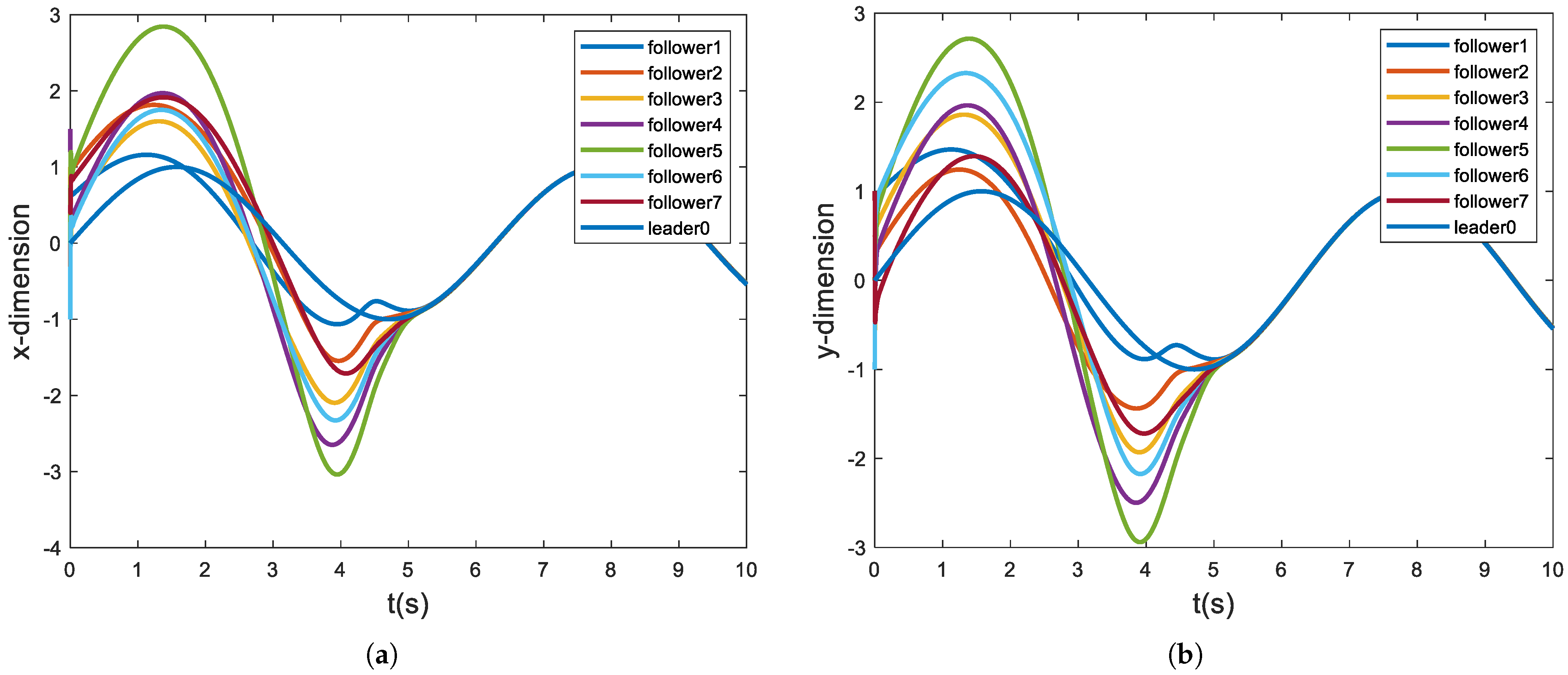Figure 6 shows the seven followers’ cumulative velocity difference converges to a bounded region. The trajectories of the agents in the x-y dimension are pictured in Figure 7, and it can be seen from the figure that all followers can follow the leader’s movements within 6 s. As demonstrated by Figure 8, the velocity of each follower is bounded, and before the appointed time, the follower’s velocity converges to the leader’s velocity, which is also consistent with the convergence of the followers’ position, as shown in Figure 7. Figure 9 further shows that the position tracking error converges to an arbitrarily small expected region within the appointed time, which verifies that the system achieves the practically leader-following appointed-time consensus.

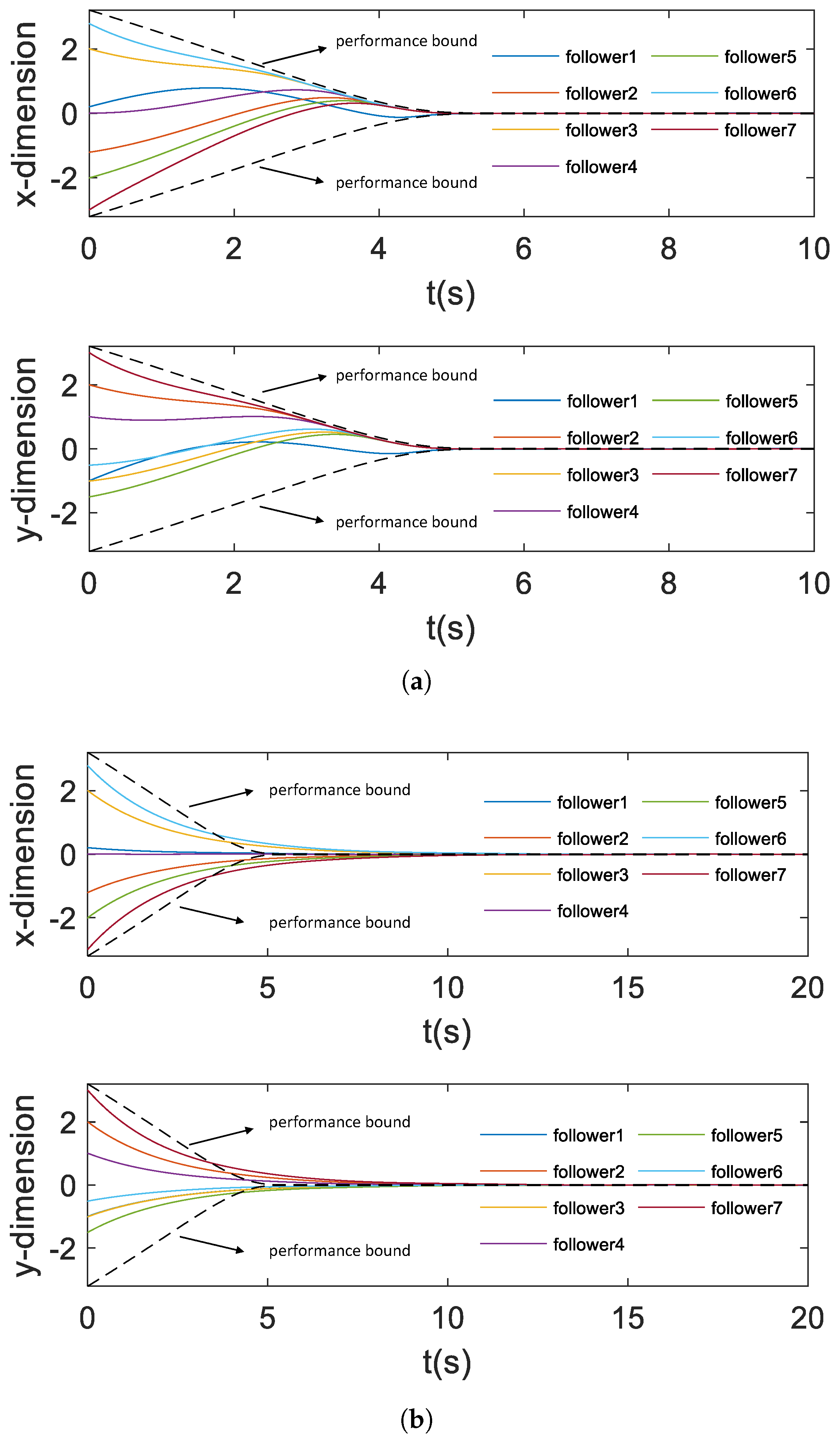
In order to analyze the sensitivities of the control parameters for the system performance, we choose different control parameters for the proposed control scheme. In both three cases, except for $k_1$ and $k_2$, all other parameters remain the same. The maximum amplitude of the control input and the control effort under different parameters on x-dimension are shown in

Table 3. Maximum control input and control effort for the proposed controller with different design parameters in x-dimension.

Parameters	Maximum Control Input	Control Effort
$k_1=24,k_2=70$	145.5	362.4
$k_1=64,k_2=150$	318.4	361.5
$k_1=120,k_2=300$	625.2	361.3

. Figure 10a,b show the cumulative position difference trajectories with controller parameters set to $k_1=24$, $k_2=70$ and $k_1=120$, $k_2=300$, respectively.

Remark 3.

As shown in Table 3, we further choose different $k_1$ and $k_2$. In all the three cases, convergence can be achieved with the similar control effort. Furthermore, as $k_1$ and $k_2$ are increased, the oscillation is reduced at the cost of increasing the control input, as shown in Figure 4a and Figure 10.

5. Conclusions and Future Works

In this paper, a distributed prescribed performance control approach is developed for second-order leader-following MASs with external disturbance under directed graphs. Compared with most of the traditional consensus control schemes which only guarantee the steady-state performance of the system, our controller can ensure that the position tracking error converges to a specified arbitrarily small expected region in appointed-time, and the cumulative position difference converges to the specified performance bound region; in other words, the transient and steady-state performance of the system are guaranteed simultaneously. In addition, the controller does not require prior knowledge of the external disturbance. It is assumed in this paper that the state of the system is measurable, and thus the proposed control method is not applicable to cases where the state is not measurable. Future research will focus on adopting event-triggered control strategies to reduce the communication resources of individual agents, and to deal with cases where the state variables of MASs are not measured.

References

1. Gul, F.; Mir, A.; Mir, I.; Mir, S.; Islaam, T.U.; Abualigah, L.; Forestiero, A. A Centralized Strategy for Multi-Agent Exploration. IEEE Access 2022, 10, 126871–126884. [Google Scholar] [CrossRef]
2. Xu, C.; Wu, B.; Wang, D. Distributed Prescribed-Time Attitude Coordination for Multiple Spacecraft With Actuator Saturation Under Directed Graph. IEEE Trans. Aerosp. Electron. Syst. 2022, 58, 2660–2672. [Google Scholar] [CrossRef]
3. Gao, S.; Dong, H.; Ning, B.; Zhang, Q. Cooperative Prescribed Performance Tracking Control for Multiple High-Speed Trains in Moving Block Signaling System. IEEE Trans. Intell. Transp. Syst. 2019, 20, 2740–2749. [Google Scholar] [CrossRef]
4. Hong, Y.; Gao, L.; Cheng, D.; Hu, J. Lyapunov-based approach to multiagent systems with switching jointly connected interconnection. IEEE Trans. Autom. Control. 2007, 52, 943–948. [Google Scholar] [CrossRef]
5. Peng, K.; Yang, Y. Leader-following consensus problem with a varying-velocity leader and time-varying delays. Phys. A Stat. Mech. Its Appl. 2009, 388, 193–208. [Google Scholar] [CrossRef]
6. Ni, W.; Cheng, D. Leader-following consensus of multi-agent systems under fixed and switching topologies. Syst. Control. Lett. 2010, 59, 209–217. [Google Scholar] [CrossRef]
7. Li, H.; Liao, X.; Huang, T.; Zhu, W. Event-triggering sampling based leader-following consensus in second-order multi-agent systems. IEEE Trans. Autom. Control 2014, 60, 1998–2003. [Google Scholar] [CrossRef]
8. Hu, W.; Yang, C.; Huang, T.; Gui, W. A distributed dynamic event-triggered control approach to consensus of linear multiagent systems with directed networks. IEEE Trans. Cybern. 2018, 50, 869–874. [Google Scholar] [CrossRef]
9. Du, C.; Liu, X.; Ren, W.; Lu, P.; Liu, H. Finite-Time Consensus for Linear Multiagent Systems via Event-Triggered Strategy Without Continuous Communication. IEEE Trans. Control. Netw. Syst. 2020, 7, 19–29. [Google Scholar] [CrossRef]
10. Mazare, M.; Asharioun, H.; Davoudi, E.; Mokhtari, M. Distributed finite-time neural network observer-based consensus tracking control of heterogeneous underwater vehicles. Ocean. Eng. 2023, 272, 113882. [Google Scholar] [CrossRef]
11. Hu, W.; Cheng, Y.; Chen, Z. Reset control for consensus of double-integrator multi-agent systems. Automatica 2022, 136, 110057. [Google Scholar] [CrossRef]
12. Cheng, Y.; Hu, W.; Guo, Y.; Xie, Y. Reset control for leader-following consensus of multi-agent systems. ISA Trans. 2022, 129, 130–139. [Google Scholar] [CrossRef] [PubMed]
13. Bechlioulis, C.P.; Rovithakis, G.A. Robust adaptive control of feedback linearizable MIMO nonlinear systems with prescribed performance. IEEE Trans. Autom. Control 2008, 53, 2090–2099. [Google Scholar] [CrossRef]
14. Bechlioulis, C.P.; Rovithakis, G.A. Adaptive control with guaranteed transient and steady state tracking error bounds for strict feedback systems. Automatica 2009, 45, 532–538. [Google Scholar] [CrossRef]
15. Han, S.I.; Lee, J.M. Improved prescribed performance constraint control for a strict feedback non-linear dynamic system. IET Control Theory Appl. 2013, 7, 1818–1827. [Google Scholar] [CrossRef]
16. Li, Y.; Tong, S.; Liu, L.; Feng, G. Adaptive output-feedback control design with prescribed performance for switched nonlinear systems. Automatica 2017, 80, 225–231. [Google Scholar] [CrossRef]
17. Kostarigka, A.K.; Doulgeri, Z.; Rovithakis, G.A. Prescribed performance tracking for flexible joint robots with unknown dynamics and variable elasticity. Automatica 2013, 49, 1137–1147. [Google Scholar] [CrossRef]
18. Guo, Q.; Zhang, Y.; Celler, B.G.; Su, S.W. Neural adaptive backstepping control of a robotic manipulator with prescribed performance constraint. IEEE Trans. Neural Netw. Learn. Syst. 2018, 30, 3572–3583. [Google Scholar] [CrossRef]
19. Hu, Q.; Shao, X.; Guo, L. Adaptive fault-tolerant attitude tracking control of spacecraft with prescribed performance. IEEE/ASME Trans. Mechatron. 2017, 23, 331–341. [Google Scholar] [CrossRef]
20. Karayiannidis, Y.; Dimarogonas, D.V.; Kragic, D. Multi-agent average consensus control with prescribed performance guarantees. In Proceedings of the 2012 IEEE 51st IEEE Conference on Decision and Control (CDC), Maui, HI, USA, 10–13 December 2012; pp. 2219–2225. [Google Scholar]
21. Macellari, L.; Karayiannidis, Y.; Dimarogonas, D.V. Multi-agent second order average consensus with prescribed transient behavior. IEEE Trans. Autom. Control 2016, 62, 5282–5288. [Google Scholar] [CrossRef]
22. Bechlioulis, C.P.; Rovithakis, G.A. Decentralized robust synchronization of unknown high order nonlinear multi-agent systems with prescribed transient and steady state performance. IEEE Trans. Autom. Control 2016, 62, 123–134. [Google Scholar] [CrossRef]
23. Zhang, L.; Hua, C.; Guan, X. Distributed output feedback consensus tracking prescribed performance control for a class of non-linear multi-agent systems with unknown disturbances. IET Control Theory Appl. 2016, 10, 877–883. [Google Scholar] [CrossRef]
24. Wang, W.; Wang, D.; Peng, Z.; Li, T. Prescribed performance consensus of uncertain nonlinear strict-feedback systems with unknown control directions. IEEE Trans. Syst. Man Cybern. Syst. 2015, 46, 1279–1286. [Google Scholar] [CrossRef]
25. Zhang, L.; Che, W.W.; Chen, B.; Lin, C. Adaptive fuzzy output-feedback consensus tracking control of nonlinear multiagent systems in prescribed performance. IEEE Trans. Cybern. 2022, 53, 1932–1943. [Google Scholar] [CrossRef]
26. Dong, G.; Ren, H.; Yao, D.; Li, H.; Lu, R. Prescribed performance consensus fuzzy control of multiagent systems with nonaffine nonlinear faults. IEEE Trans. Fuzzy Syst. 2020, 29, 3936–3946. [Google Scholar] [CrossRef]
27. Cortés, J. Finite-time convergent gradient flows with applications to network consensus. Automatica 2006, 42, 1993–2000. [Google Scholar] [CrossRef]
28. Xiao, F.; Wang, L.; Chen, T. Finite-time consensus in networks of integrator-like dynamic agents with directional link failure. IEEE Trans. Autom. Control 2013, 59, 756–762. [Google Scholar] [CrossRef]
29. Fu, J.; Wen, G.; Yu, W.; Ding, Z. Finite-time consensus for second-order multi-agent systems with input saturation. IEEE Trans. Circuits Syst. II Express Briefs 2017, 65, 1758–1762. [Google Scholar] [CrossRef]
30. Hong, H.; Yu, W.; Fu, J.; Yu, X. Finite-time connectivity-preserving consensus for second-order nonlinear multiagent systems. IEEE Trans. Control. Netw. Syst. 2018, 6, 236–248. [Google Scholar] [CrossRef]
31. Zuo, Z. Nonsingular fixed-time consensus tracking for second-order multi-agent networks. Automatica 2015, 54, 305–309. [Google Scholar] [CrossRef]
32. Huang, Y.; Jia, Y. Fixed-time consensus tracking control for second-order multi-agent systems with bounded input uncertainties via NFFTSM. IET Control Theory Appl. 2017, 11, 2900–2909. [Google Scholar] [CrossRef]
33. Wen, G.X.; Chen, C.P.; Liu, Y.J.; Liu, Z. Neural-network-based adaptive leader-following consensus control for second-order non-linear multi-agent systems. IET Control Theory Appl. 2015, 9, 1927–1934. [Google Scholar] [CrossRef]
34. Wang, W.; Wang, D.; Peng, Z. Cooperative fuzzy adaptive output feedback control for synchronisation of nonlinear multi-agent systems under directed graphs. Int. J. Syst. Sci. 2015, 46, 2982–2995. [Google Scholar] [CrossRef]
35. Wei, C.; Luo, J.; Yin, Z.; Yuan, J. Leader-following consensus of second-order multi-agent systems with arbitrarily appointed-time prescribed performance. IET Control Theory Appl. 2018, 12, 2276–2286. [Google Scholar] [CrossRef]
36. Qu, Z. Cooperative Control of Dynamical Systems: Applications to Autonomous Vehicles; Springer Science & Business Media: Berlin/Heidelberg, Germany, 2009. [Google Scholar]
37. Horn, R.A.; Horn, R.A.; Johnson, C.R. Topics in Matrix Analysis; Cambridge University Press: Cambridge, UK, 1994. [Google Scholar]
38. Gao, S.; Li, M.; Zheng, Y.; Zhao, N.; Dong, H. Fuzzy Adaptive Protective Control for High-Speed Trains: An Outstretched Error Feedback Approach. IEEE Trans. Intell. Transp. Syst. 2022, 23, 17966–17975. [Google Scholar] [CrossRef]
39. Liu, Y.; Liu, X.; Jing, Y. Adaptive fuzzy finite-time stability of uncertain nonlinear systems based on prescribed performance. Fuzzy Sets Syst. 2019, 374, 23–39. [Google Scholar] [CrossRef]
40. Shivakumar, P.; Chew, K.H. A sufficient condition for nonvanishing of determinants. Proc. Am. Math. Soc. 1974, 43, 63–66. [Google Scholar] [CrossRef]
Figure 1. Error transformation: (a) case of e ( 0 ) 0 , and (b) case of e ( 0 ) < 0 .
Applsci 13 05937 g001
Figure 2. Consensus control block diagram for each follower i.
Applsci 13 05937 g002
Figure 3. Topology in the simulation.
Applsci 13 05937 g003
Figure 4. The evolution of seven followers’ cumulative position difference on x-dimension and y-dimension with performance bounds (dashed lines) with t f = 6 s. (a) Case of the consensus protocol with PPC and d ( t ) 0 . (b) Case of the consensus protocol without PPC and d ( t ) 0 .
Applsci 13 05937 g004
Figure 5. The evolution of seven followers’ cumulative position difference on x-dimension with t f = 6 s . (a) Case of the proposed protocol (14). (b) Case of the protocol (31).
Applsci 13 05937 g005
Figure 6. The evolution of seven followers’ cumulative velocity difference on x-dimension and y-dimension.
Applsci 13 05937 g006
Figure 7. Trajectory of the agents in the x–y dimension.
Applsci 13 05937 g007
Figure 8. The evolution of the velocity of seven followers and one leader: (a) x-dimension and (b) y-dimension.
Applsci 13 05937 g008
Figure 9. The evolution of seven followers’ position tracking error with t f = 6 s .
Applsci 13 05937 g009
Figure 10. The evolution of seven followers’ cumulative position difference on x-dimension and y-dimension with performance bounds (dashed lines) with t f = 6 s . (a) Case of the PPC controller with k 1 = 24 , k 2 = 70 . (b) Case of the PPC controller with k 1 = 120 , k 2 = 300 .
Applsci 13 05937 g010