A Partitioned Rigid-Element and Interface-Element Method for Rock-Slope-Stability Analysis

Abstract

The stability analysis of rock slopes has been a prominent topic in the field of rock mechanics, primarily due to the widespread occurrence of discontinuous structural planes in rock masses. Based on this complex characteristic of rock slopes, this paper proposes a novel numerical method, the Partitioned-Rigid-Element and Interface-Element (PRE-IE) method. In the PRE-IE method, the structure is modeled as several rigid bodies and discontinuous structural planes, which are, respectively, divided into partitioned rigid elements and interface elements. Taking the contact force of node pairs and the displacement of the rigid body centroid as mixed variables, according to the principle of minimum potential energy, the governing equations of PRE-IE can be established using the Lagrange multiplier method and then solved using the nonlinear contact iterative method and the incremental method. A classic case study demonstrates that using the failure of all contact node pairs as the criterion for slope failure is appropriate. This criterion is objective and avoids the potential impact of personal bias on safety factor calculations. Two numerical examples of differently shaped slopes are provided to verify the correctness and validity of the PRE-IE method. By comparing the safety factor calculated using the PRE-IE method with those obtained from other different methods, as well as comparing the computational time, it is shown that the PRE-IE method, in combination with the SRM, can accurately and efficiently analyze the stability problems of rock slopes.

1. Introduction

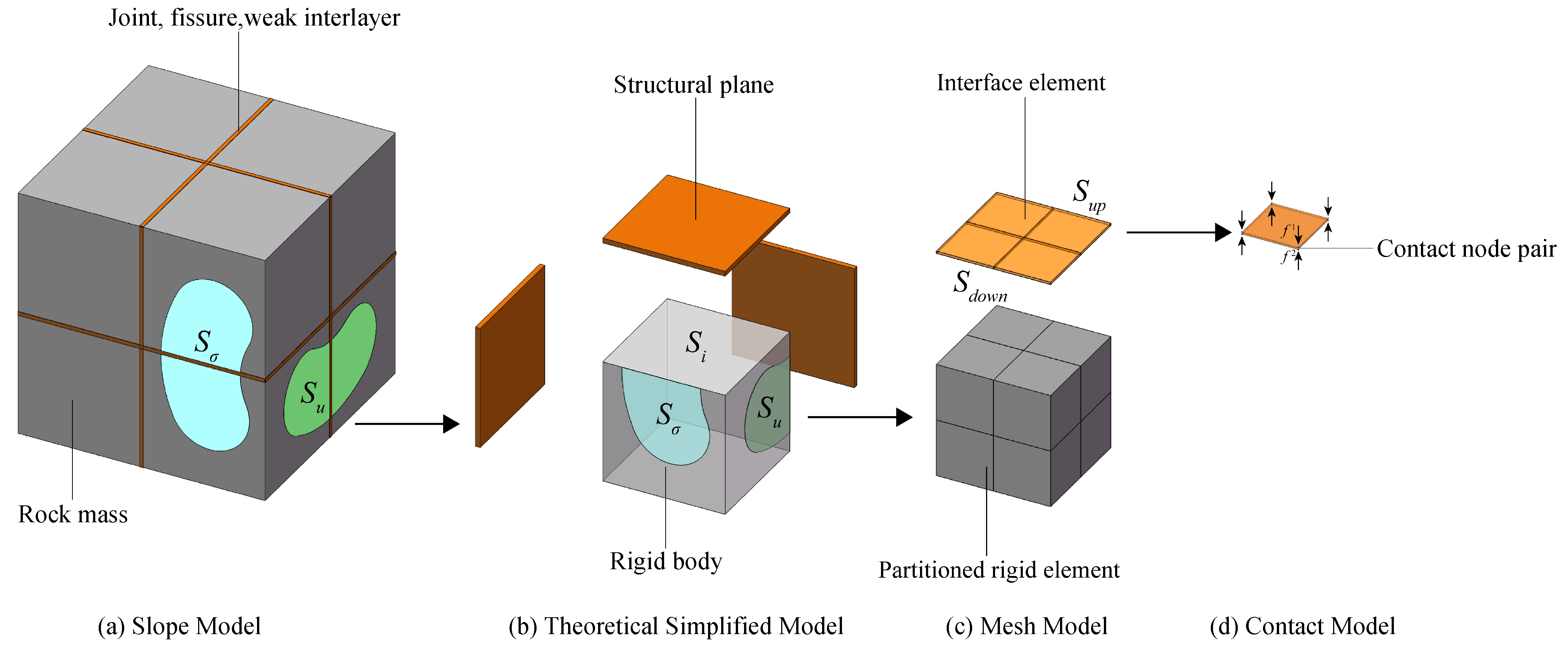
In recent years, China has planned to establish numerous water conservancy and hydropower projects in the southwest. In these areas, there may be a large number of rock slopes with complex structures and frequent geotectonic movements, which can cause serious consequences for nearby facilities in case of landslides or earthquakes. Therefore, ensuring the stability of rock slopes is crucial for the long-term safe and effective operation of engineering projects. Rock slopes often contain many discontinuous structural planes, such as joints, fissures, and weak interlayers. As a result, the slope can be viewed as consisting of two distinct structures: the rock masses segmented by structural planes, which collectively form a continuous medium, and the discontinuous structural planes themselves, characterized by their irregular shapes, thinness, and vastly different mechanical properties compared to the adjacent rock masses. As such, the structural plane becomes a potential slip surface during slope failure. Therefore, in order to study and analyze the failure mechanism of rock slope, it is necessary to explore innovative methods and conduct in-depth research on the nonlinear and discontinuous characteristics of the structural planes.

The commonly used methods for slope-stability analysis are the limit equilibrium method (LEM) [1,2,3], limit analysis method (LAM) [4,5], and other numerical methods. The first two methods are based on the assumption of elastic and perfectly plastic material or rigid and perfectly plastic material, ignoring the loading process and only considering the ultimate load at the time of structural failure. Therefore, they are mostly used for simple two-dimensional problems, are not suitable for solving complex three-dimensional problems, and cannot simulate the process of slope transformation from continuous-medium to discontinuous-medium when slope failure occurs. With the popularization of computers and the improvement in computational efficiency, the use of numerical methods to analyze slope stability has gradually become mainstream [6]. These numerical methods can not only satisfy the mechanical equilibrium conditions while considering the nonlinear constitutive relation of materials, but also demonstrate the development process of the plastic zone during slope failure, which is suitable for solving slope problems with complex conditions.

Since Zienkiewicz [7] proposed the finite-element method–strength-reduction-method (FEM-SRM) in 1975, FEM has gradually become a popular numerical method for slope-stability analysis [8,9,10]. Lin et al. [11] constructed a 3D slope model by extending the 2D model longitudinally to study the effects of the dilatancy angle using the PLAXIS 3D FEM with the built-in strength reduction technique. The results showed that the effects of the dilatancy angle on the convergence of 3D and 2D slope models are different. Liu et al. [12] proposed a 2D and 3D slope-stability finite-element limit equilibrium method using elastic finite-element stress fields and indicated that FEM can be applied to solve various slope problems. The FEM also introduces a large number of special elements (such as joint element [13,14], and thin layer element [15,16]) to simulate the nonlinear characteristics of the slope structural plane. However, this will put forward a high requirement for meshing, which not only requires the mesh near the discontinuity to be dense enough to ensure the computational accuracy, but also requires the mesh of ordinary elements and special elements to satisfy the compatibility condition on the boundary. Furthermore, in the dynamic case, despite the introduction of special elements, the elastic–plastic constitutive relationship adopted by the finite element makes it difficult to simulate the stick and debonding of discontinuous interfaces. Moreover, in the calculation process, the stiffness matrix of the whole region needs to be updated even if the nonlinear relationship only appears in the local region. Therefore, the conventional FEM is inefficient in solving complicated discontinuity issues. In 1999, Belytschko [17] proposed a minimal remeshing finite-element method for crack growth. This method allows the crack to be arbitrarily aligned within the mesh. For severely curved cracks, remeshing may be needed, but only away from the crack tip, where remeshing is much easier. Then it evolved into a novel method called the extended finite element method (XFEM) and has subsequently been developed quickly worldwide. XFEM can be used to simulate heterogeneous materials with voids and inclusions, interfaces of bimaterial, and two-phase, so it is a possible computational alternative to treat slope instability, concrete cracking, and interfacial problems [18].

With the in-depth study of numerical methods, the numerical methods based on the continuous medium hypothesis can hardly meet the requirements of researchers for calculation accuracy, and the numerical simulation of complex structural planes in the rock slope has gradually developed into discontinuous medium methods. The continuum medium method is dominated by FEM, and the discontinuous medium method is dominated by the discrete element method (DEM) [19] and discontinuous deformation analysis (DDA) [20]. Jiang et al. [21] presented a numerical investigation into the rainfall-induced instability mechanism of a jointed rock slope with two joint inclinations of dipping 45° and 60° and the corresponding safety factor using the two-dimensional DEM, where the non-uniform strength reduction approach is employed. The results show that the proposed DEM strength reduction provides a feasible approach to analyze the rainfall-triggered instability of the jointed rock slope. Gong et al. [22] took an anti-dip layered rock slope supported with anchor cables that failed owing to flexural toppling as an example, and took the DDA as the main analytical tool. The rationality of DDA was verified by correctly simulating the failure state of the anti-layered rock slope, and the underlying failure mechanism was studied. In recent years, the coupled FEM-DEM approach [23] has been widely used. In this method, DEM is used in the discontinuous medium region and FEM is used in the continuous medium region, and the two regions are connected by defining a special transition layer, which can be used to simulate the failure process of local discontinuous and heterogeneous structures. However, DEM and DDA have the following limitations in practical use: DEM and DDA can usually only simulate two-dimensional models or simple three-dimensional models; these two methods require many mechanical and kinematic parameters to be determined before calculation, but the relationship between these parameters and the macroscopic properties of object is not clear; and most importantly, the DEM and DDA have high requirements for computer performance and are time-consuming when solving large and complex slope stability problems.

The rigid element method (REM) [24,25] is another numerical method that can simulate structural planes in rock slopes. The REM regards the system as a mass of rigid elements connected by springs distributed on contact surfaces, and the strain energy of the structure is only stored at the interface between the rigid elements. Compared with FEM, REM can solve the problems of cracking, dislocation, and sliding between elements. Compared with DEM and DDA, the computational efficiency is greatly improved. However, since the displacement interpolation function of REM is first-order, the displacement has only first-order approximation. In addition, the node stress cannot be obtained directly by REM, but only indirectly by the surface force on the interface. Therefore, the accuracy of displacement and stress solved by REM is low, which makes it difficult apply to practical slope stability analysis.

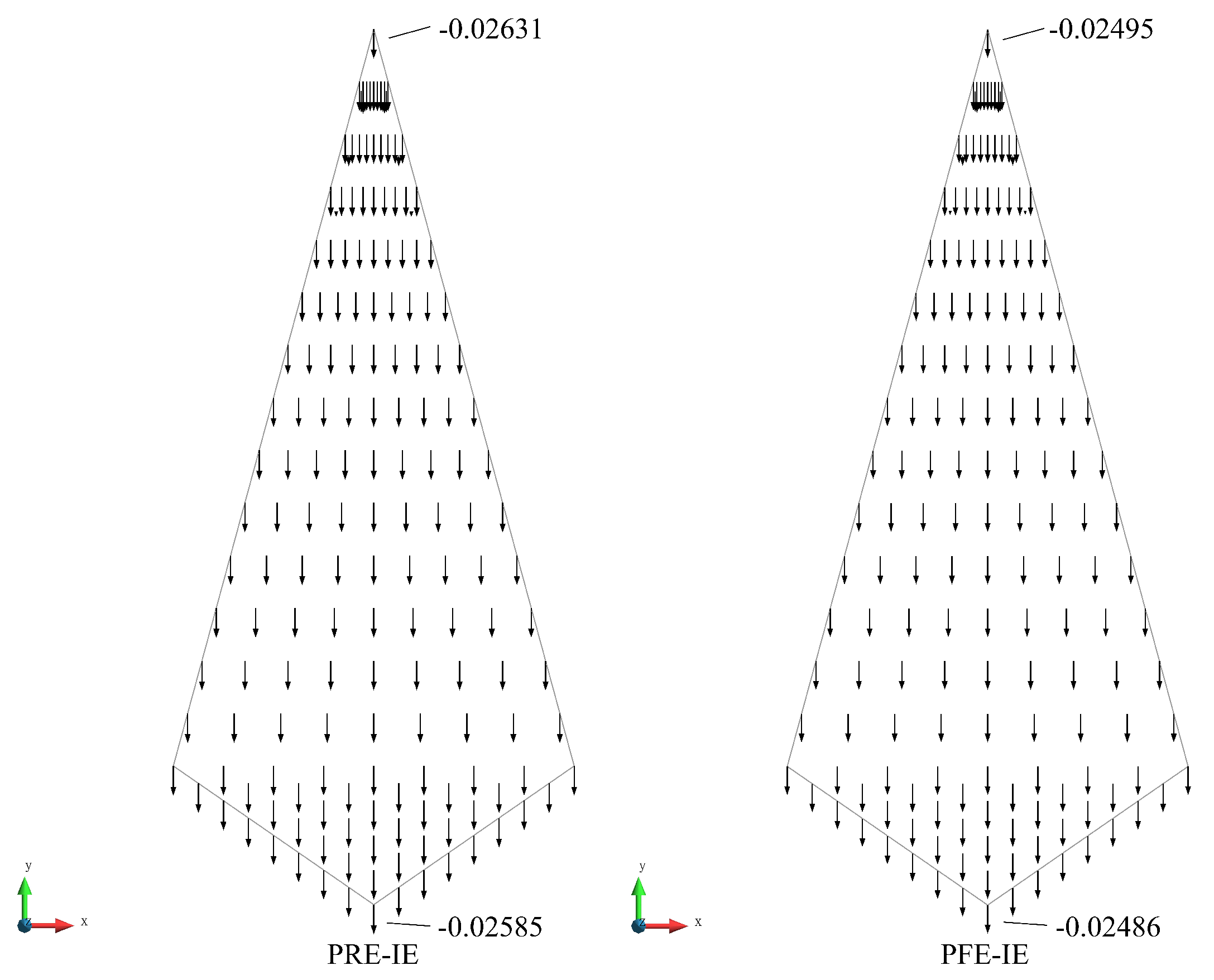
To solve such problems as slope instability, concrete cracking, and opening or closing of internal contraction joints in the dam, Li [26] proposed an interactive method of partitioned finite elements and interface elements (PFE-IE). This method divides the structure into several continuous and locally discontinuous interfaces. Treating nodal displacement as a variable, the elastic deformation of the continuum is solved using PFE, and the rigid displacements in each body and the constraining internal forces on the interface are solved using IE based on the continuous stress condition and the static force equilibrium condition. The PFE-IE method absorbs the advantages of FEM, DEM, and DDA and partitions the large-scale model with structural discontinuity and nonlinear mechanical properties so that each region can be solved independently and the solution speed can be improved. Moreover, the PFE-IE method can conveniently calculate the stability safety factor of rock slopes with the SRM [27].

With PFE-IE method, most of the time is spent solving the stiffness matrix of the elastic body in the slope. However, in practice, when the rock slope is in the limit equilibrium state, the elastic deformation of the rock mass can be ignored compared with the deformation at the structural plane. Therefore, we would like to find a new method to treat the rock mass as a rigid body, which can greatly improve the computational speed with less impact on the calculation accuracy.

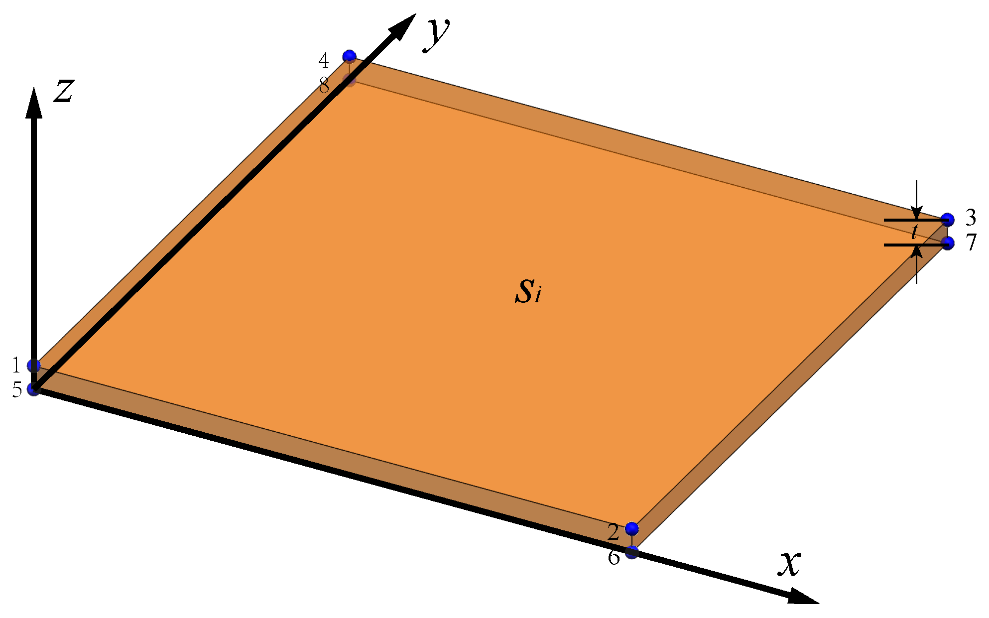
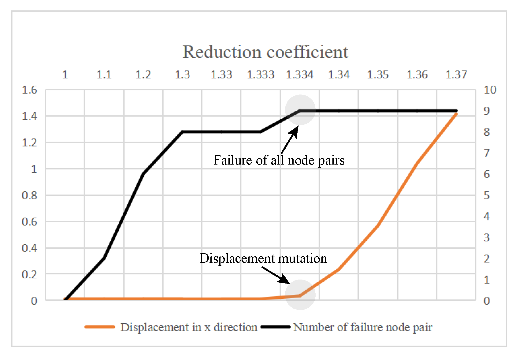
In this paper, the partitioned rigid elements and interface elements (PRE-IE) method is proposed as an improvement to the existing PFE-IE method: the structure is divided into several rigid bodies and discontinuous structural planes, on which the partitioned rigid element and interface element are established, respectively, so that the contact forces and displacements on the nodes between the rigid elements and the corresponding interface elements can be coupled. By taking the contact force of node pairs and the displacement of the rigid body centroid as mixed variables, the Lagrange multiplier method is used to establish a potential energy functional according to the principle of minimum potential energy. Then, the governing equations of PRE-IE are obtained through variational calculus and solved using the nonlinear contact iterative method and the incremental method. Finally, taking the failure of all contact node pairs as the criterion of slope failure, the stability safety factor of rock slope can be calculated using SRM. PRE-IE method absorbs the advantages of PFE-IE method and only performs nonlinear iteration on possible discontinuous structural planes, which greatly improves the efficiency of numerical calculation.

The PFE-IE method can be applied to analyze the dynamic stability of a high steep rock slope [28,29] and can be coupled with the smoothed particle hydrodynamics (SPH) method to investigate the effects of a landslide-generated wave (LGW) for the the safety of reservoir areas [30]. As an improvement to the PFE-IE method, the PRE-IE method also has the potential to solve these problems. Therefore, future research could focus on using the PRE-IE method to analyze the dynamic behaviors of structures such as slopes, dams, and retaining walls and investigate the coupling of the PRE-IE method with other emerging methods [31,32] to monitor the stability of reservoir bank slopes and the structural health of dams.

2. Theory

A schematic diagram of the PRE-IE method is shown in Figure 1:

(a)

There are a large number of joints, fissures, and weak interlayers in the rock slope.

(b)

The rock masses are considered as a rigid body, which are connected by discontinuous structural planes between them. The thicknesses of structural planes are much smaller than the geometric sizes of adjacent rock masses.

(c)

The interface elements are divided on the structure planes, and the corresponding rigid elements are partitioned, so that the contact forces and displacements of nodes on the contact interface can be coupled.

(d)

The contact node pair can be used to transfer the contact force and judge the contact mode.

The main theory of the PRE-IE method is based on the innovative modifications of the PFE-IE method [33], as detailed below.

2.1. Equations of Rigid Element

As shown in Figure 1b, The boundary of the rigid element consists of three parts: the stress boundary $S_{\mathit{\sigma }}$, the displacement boundary $S_u$, and the interface boundary $S_i$. Since there is no deformation inside the rigid element, the strain is 0. According to the principle of virtual displacement, the equivalent integral weak form of equilibrium equations and boundary conditions of the rigid element can be obtained, which has the following matrix expression:

$${\int }_{S_{\mathit{\sigma }}}\delta {\mathit{u}}^T\mathit{t}\mathrm{d}S+{\int }_{S_i}\delta {\mathit{u}}^T\mathit{F}\mathrm{d}S+{\int }_V\delta {\mathit{u}}^T{\mathit{f}}_g\mathrm{d}V=0$$

(1)

where $\delta \mathit{u}$ is the virtual displacement, $\mathit{t}$ is the surface force on the $S_{\mathit{\sigma }}$, $\mathit{F}$ is the surface force on the $S_i$, ${\mathit{f}}_g$ is the body force, and V is the integral region of the rigid element. According to the principle of minimum potential energy, Equation (1) can be expressed as

$$\delta {\Pi }_P^r=0$$

(2)

where ${\Pi }_P^r$ is the potential energy of a rigid element, which can be expressed as

$${\Pi }_P^r={\int }_{S_{\mathit{\sigma }}}{\mathit{u}}^T\mathit{t}\mathrm{d}S+{\int }_{S_i}{\mathit{u}}^T\mathit{F}\mathrm{d}S+{\int }_V{\mathit{u}}^T{\mathit{f}}_g\mathrm{d}V$$

(3)

The displacement $\mathit{u}$ of any node on a rigid element can be expressed as

$$\mathit{u}=\left[\begin{array}{c}{u}_x\hfill \\ u_y\hfill \\ u_z\hfill \end{array}\right]=\left[\begin{array}{cccccc}1& 0& 0& 0& z-z_c& y_c-y\\ 0& 1& 0& z_c-z& 0& x-x_c\\ 0& 0& 1& y-y_c& x_c-x& 0\end{array}\right]\left[\begin{array}{c}{u}_x^c\\ u_y^c\\ u_z^c\\ {\theta }_x^c\\ {\theta }_y^c\\ {\theta }_z^c\end{array}\right]=\mathit{W}{\mathit{\gamma }}^e$$

(4)

where $\mathit{W}$ is the rigid displacement transformation matrix, ${\gamma }^e$ is the displacement of the rigid body centroid, and $\left(x_c,y_c,z_c\right)$ is the coordinates of the rigid body centroid. Substituting Equation (4) into Equation (3), the potential energy of rigid element can be written as follows:

$${\Pi }_P^r={\int }_{S_{\mathit{\sigma }}}{\mathit{\gamma }}^{e^T}{\mathit{W}}^T\mathit{t}\mathrm{d}S+{\int }_{S_i}{\mathit{\gamma }}^{e^T}{\mathit{W}}^T\mathit{F}\mathrm{d}S+{\int }_V{\mathit{\gamma }}^{e^T}{\mathit{W}}^T{\mathit{f}}_g\mathrm{d}V$$

(5)

2.2. Equations of Interface Element

Since the use of non-thickness joint elements may cause the adjacent rigid elements to overlap, PRE-IE uses thin-layer elements as interface elements [15,16] (as shown in Figure 1c). In this paper, we take the eight-node hexahedral thin-layer element shown in Figure 2 as an example. The thickness of the interface element is t, and the mass force is negligible. According to the principle of virtual displacement, the equivalent integral weak form of equilibrium equations and boundary conditions of the interface element can be obtained, which has the following matrix expression:

$${\int }_{\Omega }\delta {\mathit{\epsilon }}^T\mathit{\sigma }\mathrm{d}V-{\int }_{S_i}\delta {\mathit{u}}^T\mathit{F}\mathrm{d}S=0$$

(6)

where $\Omega$ is the integral region of the interface element, $\mathit{\epsilon }$ and $\mathit{\sigma }$ are the stress and strain inside the interface, and $\mathit{F}$ is the surface force on the $S_i$. According to the principle of minimum potential energy, Equation (6) can be expressed as

$$\delta {\Pi }_P^i=0$$

(7)

where ${\Pi }_P^i$ is the potential energy of the rigid element, which can be expressed as

$${\Pi }_P^i=\frac{1}{2}{\int }_{\Omega }{\epsilon }^T\mathit{\sigma }\mathrm{d}V-{\int }_{S_i}{\mathit{u}}^T\mathit{F}\mathrm{d}S$$

(8)

${\mathit{u}}_{up}$ is the displacement of any point on the upper surface of the interface element, and ${\mathit{u}}_{down}$ is the nodal displacement, the displacement of any point on the lower surface of the interface element, which can be expressed as follows:

$${\mathit{u}}_{up}={\mathit{N}}_1{\mathit{u}}_1+{\mathit{N}}_2{\mathit{u}}_2+{\mathit{N}}_3{\mathit{u}}_3+{\mathit{N}}_4{\mathit{u}}_4=\mathit{N}{\mathit{a}}_{up}^e$$

(9)

$${\mathit{u}}_{down}={\mathit{N}}_1{\mathit{u}}_5+{\mathit{N}}_2{\mathit{u}}_6+{\mathit{N}}_3{\mathit{u}}_7+{\mathit{N}}_4{\mathit{u}}_8=\mathit{N}{\mathit{a}}_{down}^e$$

(10)

where $\mathit{N}$ is the shape function matrix of the four-node quadrilateral isoparametric element, $\mathit{u}$ is the nodal displacement, ${\mathit{a}}_{up}^e$ is the nodal displacement array on the upper surface of the interface element, and ${\mathit{a}}_{down}^e$ is the nodal displacement array on the lower surface of the interface element.

Then, the displacement difference between upper and lower surfaces $\Delta \mathit{u}$ can be expressed as

$$\Delta \mathit{u}=\left[\begin{array}{c}\Delta u_x\\ \Delta u_y\\ \Delta u_z\end{array}\right]={\mathit{u}}_{up}-{\mathit{u}}_{down}=\mathit{B}{\mathit{a}}^e$$

(11)

where $\mathit{B}$ is the shape function matrix of the interface element and ${\mathit{a}}^e$ is the nodal displacement array of the interface element, which can be expressed as follows:

$$B=\left[\begin{array}{cccccccc}{\mathit{N}}_1\hfill & {\mathit{N}}_2\hfill & {\mathit{N}}_3\hfill & {\mathit{N}}_4\hfill & -{\mathit{N}}_1\hfill & -{\mathit{N}}_2\hfill & -{\mathit{N}}_3\hfill & -{\mathit{N}}_4\hfill \end{array}\right]$$

(12)

$${\mathit{a}}^e=\left[\begin{array}{c}{\mathit{u}}_1\hfill \\ {\mathit{u}}_2\hfill \\ {\mathit{u}}_3\hfill \\ {\mathit{u}}_4\hfill \\ {\mathit{u}}_5\hfill \\ {\mathit{u}}_6\hfill \\ {\mathit{u}}_7\hfill \\ {\mathit{u}}_8\hfill \end{array}\right]=\left[\begin{array}{c}{\mathit{a}}_{up}^e\\ {\mathit{a}}_{\mathrm{down}}^e\end{array}\right]$$

(13)

Since the element thickness t is small compared to the whole structure, there are only tangential strains ${\gamma }_{zx}$ and ${\gamma }_{zy}$ parallel to the interface and normal strain ${\epsilon }_z$ perpendicular to the interface in the interface element. The strain $\epsilon$ is related to the displacement difference $\Delta \mathit{u}$ and is constant in the thickness direction, which can be expressed as follows:

$$\mathit{\epsilon }=\left[\begin{array}{c}{\mathit{\gamma }}_{zx}\hfill \\ {\mathit{\gamma }}_{zy}\hfill \\ {\epsilon }_z\hfill \end{array}\right]=\left[\begin{array}{c}\frac{\Delta u_x}{t}\\ \frac{\Delta u_y}{t}\\ \frac{\Delta u_z}{t}\end{array}\right]=\frac{\Delta \mathit{u}}{t}$$

(14)

the stress $\mathit{\sigma }$ can be expressed as:

$$\mathit{\sigma }=\left[\begin{array}{c}{\tau }_{zx}\\ {\tau }_{zy}\\ {\sigma }_z\end{array}\right]=\left[\begin{array}{ccc}t{k}_{xx}& 0& 0\\ 0& t{k}_{yy}& 0\\ 0& 0& t{k}_{zz}\end{array}\right]\left[\begin{array}{c}{\mathit{\gamma }}_{zx}\\ {\mathit{\gamma }}_{zy}\\ {\epsilon }_z\end{array}\right]=\mathit{D}\mathit{\epsilon }$$

(15)

where $\mathit{D}$ is the elastic matrix of the structural plane, $k_{zz}$ is the normal stiffness, and $k_{xx}$ and $k_{yy}$ are the tangential stiffnesses.

Substituting Equations (11), (14) and (15) into Equation (8), the potential energy of the interface element can be written as follows:

$$\begin{array}{cc}\hfill {\Pi }_P^i& =\frac{1}{2}{\int }_{\Omega }{\mathit{\epsilon }}^T\mathit{D}\epsilon \mathrm{d}V-{\int }_{S_i}{\mathit{u}}^T\mathit{F}\mathrm{d}S\hfill \\ \hfill & =\frac{1}{2}{\int }_{\Omega }\frac{1}{{\mathit{t}}^2}\Delta {\mathit{u}}^T\mathit{D}\Delta \mathit{u}\mathrm{d}V-{\int }_{S_i}{\mathit{a}}^{e^T}{\mathit{N}}^T\mathit{F}\mathrm{d}S\hfill \\ \hfill & =\frac{1}{2}{\int }_{\Omega }\frac{1}{{\mathit{t}}^2}{\mathit{a}}^{e^T}{\mathit{B}}^T\mathit{D}\mathit{B}{\mathit{a}}^e\mathrm{d}V-{\int }_{S_i}{\mathit{a}}^{e^T}{\mathit{N}}^T\mathit{F}\mathrm{d}S\hfill \end{array}$$

(16)

2.3. Equations of PRE-IE

In order to make the force and displacement of the rigid element and interface element transfer correctly on the contact surface, the rigid element is partitioned so that the rigid element and interface element have corresponding nodes on the contact surface (as shown in Figure 1c). It is also necessary to make the following assumptions about the distribution modes of contact force and nodal displacement so that the force and displacement of the rigid element and the interface element can be coupled on the contact surface:

$${\mathit{a}}^e=\mathit{W}{\mathit{\gamma }}^{e}on{S}_i$$

(17)

$$\mathit{F}={\mathit{N}}_p{\mathit{f}}^{e}on{S}_i$$

(18)

where ${\mathit{N}}_p$ is the interpolation function matrix. By setting different interpolation functions, the contact force can be interpolated to obtain the linear distribution, quadratic distribution, or other forms of distribution surface force. In the following numerical examples, the surface forces are assumed to be linearly distributed. ${\mathit{f}}^e$ is the contact force array of contact node pairs on the interface element.

By combining Equations (5) and (16), the potential energy equation of PRE-IE can be obtained. By taking Equations (17) and (18) as constraint conditions, using the Lagrange multiplier method, the modified functional equation as shown below can be obtained:

$$\begin{array}{cc}\hfill {\Pi }_P^e& ={\int }_{S_{\mathit{\sigma }}}{\mathit{\gamma }}^{e^T}{\mathit{W}}^T\mathit{t}\mathrm{d}S+{\int }_{S_i}{\mathit{\gamma }}^{e^T}{\mathit{W}}^T\mathit{F}\mathrm{d}S+{\int }_V{\mathit{\gamma }}^{e^T}{\mathit{W}}^T{\mathit{f}}_g\mathrm{d}V\hfill \\ \hfill & +\frac{1}{2}{\int }_{\Omega }\frac{1}{{\mathit{t}}^2}{\mathit{a}}^{e^T}{\mathit{B}}^T\mathit{D}\mathit{B}{\mathit{a}}^e\mathrm{d}V-{\int }_{S_i}{\mathit{a}}^{e^T}{\mathit{N}}^T\mathit{F}\mathrm{d}S\hfill \\ \hfill & +{\int }_{S_i}\lambda \left({\mathit{a}}^e-\mathit{W}{\mathit{\gamma }}^e\right)\mathrm{d}S+{\int }_{S_i}\mu \left(\mathit{F}-{\mathit{N}}_p{\mathit{f}}^e\right)\mathrm{d}S\hfill \end{array}$$

(19)

The total potential energy ${\Pi }_P$ of a structure is the sum of the potential energy of each element:

$${\Pi }_P=\sum _e{\Pi }_P^e$$

(20)

The above equation requires that the order of each matrix in the element is the same as that in the overall structure, so the following transformation matrix needs to be introduced:

$${\mathit{f}}^e={\mathit{G}}_f\mathit{f}$$

(21)

$${\mathit{\gamma }}^e={\mathit{G}}_{\mathit{\gamma }}\gamma$$

(22)

where ${\mathit{G}}_f$ and ${\mathit{G}}_{\gamma }$ are the transformation matrixes, $\mathit{f}$ is the contact force array of overall structure, and $\mathit{\gamma }$ is the rigid displacement array of the overall structure.

The governing equation of PRE-IE shown below can be obtained from Equation (20) by using the variational calculus:

$$\left[\begin{array}{cc}{\mathit{K}}_{ff}\hfill & {\mathit{K}}_{f\mathit{\gamma }}\hfill \\ {\mathit{K}}_{\mathit{\gamma }f}\hfill & {\mathit{K}}_{\mathit{\gamma }\mathit{\gamma }}\hfill \end{array}\right]\left[\begin{array}{c}\mathit{f}\hfill \\ \mathit{\gamma }\hfill \end{array}\right]=\left[\begin{array}{c}\mathit{0}\hfill \\ \mathit{P}\hfill \end{array}\right]$$

(23)

where

$${\mathit{K}}_{ff}=-\sum _e{\int }_{S_i}{\mathit{G}}_{\mathit{\gamma }}{}^T{\mathit{W}}^T{\mathit{N}}^T{\mathit{N}}_p{\mathit{G}}_f\mathrm{d}S$$

(24)

$${\mathit{K}}_{f\mathit{\gamma }}=\sum _e{\int }_{\Omega }\frac{1}{{\mathit{t}}^2}{\mathit{G}}_{\mathit{\gamma }}{}^T{\mathit{W}}^T{\mathit{B}}^T\mathit{D}\mathit{BW}{\mathit{G}}_{\mathit{\gamma }}\mathrm{d}V$$

(25)

$${\mathit{K}}_{\mathit{\gamma }f}=-\sum _e{\int }_{S_i}{\mathit{G}}_{\mathit{\gamma }}{}^T{\mathit{W}}^T{\mathit{N}}_p{\mathit{G}}_f\mathrm{d}S$$

(26)

$${\mathit{K}}_{\mathit{\gamma }\mathit{\gamma }}=\mathit{0}$$

(27)

$$\mathit{P}=\sum _e\left({\int }_{S_{\mathit{\sigma }}}{\mathit{G}}_{\mathit{\gamma }}^T{\mathit{W}}^T\mathit{t}\mathrm{d}S+{\int }_V{\mathit{G}}_{\mathit{\gamma }}^T{\mathit{W}}^T{\mathit{f}}_g\mathrm{d}V\right)$$

(28)

The contact force $\mathit{f}$ and rigid displacement $\mathit{\gamma }$ can be obtained by solving the Equation (23).

2.4. Nonlinear Contact Iterative Method

The change in nodal displacement on a discontinuous interface will change the contact mode of the node pair (as shown in Figure 1d), and the change in the contact mode will lead to a change in the contact force; furthermore, the change in the contact force will affect the constitutive relation of interface material. This nonlinear problem can be solved using the contact iterative method below, and the contact model is shown in Figure 3. $\xi \eta \zeta$ is the local coordinate system of the contact node pair, ${\mathit{f}}^1$ and ${\mathit{f}}^2$ are the contact forces of any contact node pair, and $\delta$ is the vertical distance between the node pair, which can be written as

$${\mathit{f}}^1=-{\mathit{f}}^2=\left(f_{\xi },f_{\eta },f_{\zeta }\right)$$

(29)

$$\delta =\left({\mathit{u}}_1-{\mathit{u}}_2\right)·\mathit{\xi }$$

(30)

where ${\mathit{u}}_1$ and ${\mathit{u}}_2$ are the nodal displacements of the contact node pair.

Assuming that the interface material is elastic and perfectly plastic, according to the Mohr–Coulomb criterion, the contact modes of node pairs can be divided in three modes, as shown in

Table 1. Definition of contact mode.

Contact Mode		Displacement Criterion	Stress Criterion
Debonding		$\delta >t+{\sigma }_t/k_{zz}$	${\mathit{f}}^1=-{\mathit{f}}^2=0$
Close	Stick	$0\le \delta \le t+{\sigma }_t/k_{zz}$	$f_{\xi }<{\sigma }_{t}A,\sqrt{f_{\zeta }^2+f_{\eta }^2}<-tan\phi f_{\xi }+Ac$
	Slip	$0\le \delta \le t+{\sigma }_t/k_{zz}$	$f_{\xi }<{\sigma }_{t}A,\sqrt{f_{\zeta }^2+f_{\eta }^2}=-tan\phi f_{\xi }+Ac$

t is the initial thickness of interface; A is the control area of contact node pair; ${\sigma }_t$, $\phi$, and c are the tensile strength, internal friction angle, and cohesion, respectively.

. When the contact force or the vertical distance between the node pair changes, the contact mode of the node pair will also change. The relevant parameters of the node pair can be modified using the operations in

Table 2. Contact mode transformation.

Contact Mode	Before Iteration	After Iteration	Modified Parameters
Debonding–close	$\delta >t+{\sigma }_t/k_{zz}$	$\delta <0$	$\delta =0$
Close–debonding	$f_{\zeta }<{\sigma }_t$ A	$f_{\zeta }>{\sigma }_{t}A$	${\mathit{f}}^1=-{\mathit{f}}^2=\mathit{s}$
Stick–slip	$f_{\xi }<{\sigma }_{t}A$	$\sqrt{f_{\zeta }^2+f_{\eta }^2}>-tan\phi f_{\xi }+Ac$	${\alpha }_1=\left|f_{\zeta }\right|/\sqrt{f_{\zeta }^2+f_{\eta }^2}$ ${\alpha }_2=\left|f_{\eta }\right|/\sqrt{f_{\zeta }^2+f_{\eta }^2}$ $f_{\zeta }={\alpha }_1\left(-tan\phi f_{\xi }+Ac\right)$ $f_{\eta }={\alpha }_2\left(-tan\phi f_{\xi }+Ac\right)$

.

Firstly, the vertical distance between the contact node pair is $\delta$, which determines whether the contact node pair is in the close or debonding mode. When the vertical distance is greater than $t+{\sigma }_t/k_{zz}$ before iteration and less than 0 after iteration, the contact mode is changed from debonding to close, and the vertical distance is modified to 0 because the node pairs cannot penetrate each other.

Next, the normal force $f_{\xi }$ is used to determine whether the contact node pair will debond or not. When the normal force is greater than the limit after iteration, the contact mode is changed from close to debonding. According to the principle that the debonding node pair cannot transfer the contact force, the contact force is modified to have a small value of $\mathit{s}$.

Then, the tangential forces $f_{\zeta }$ and $f_{\eta }$ are used to determine whether the contact node pair will slip or not. When the node pair is in the stick mode and does not yield before the iteration and then yields after the iteration, the contact mode changes from stick to slip, and the tangential forces are modified according to the Mohr–Coulomb criterion.

When the contact node pair is in the close mode, according to the equivalent deformation, the normal stiffness $k_{zz}$ can be taken as $E/t$, where E is the elasticity modulus of the structural plane based on the test and t is the thickness of the interface. However, the normal compression deformation is not the main cause of slope failure, and to prevent the excessive interpenetration of the node pair and ensure the normal displacement coordination of the rigid element and interface element on the contact surface, the normal stiffness can be taken as a value according to experience, such as $k_{zz}={10}^7\mathrm{kN}/{\mathrm{m}}^3$. When the contact node pair is in the debonding mode, a small value of $k_{zz}$ is taken as the normal stiffness, such as $k_{zz}=10\mathrm{kN}/{\mathrm{m}}^3$.

Different nonlinear elastic models can be used for tangential stiffness $k_{xx}$ and $k_{yy}$ according to the mechanical properties of the structural plane. The following Clough–Duncan hyperbolic model [6] is used for the numerical examples in this paper (assuming that the tangential modulus is isotropic):

$$k_{xx}=k_{yy}=k_1{\gamma }_w{\left(\frac{{\sigma }_n}{P_a}\right)}^n{\left(1-\frac{R_f\tau }{{\sigma }_{n}tan{\phi }_1}\right)}^2$$

(31)

where ${\gamma }_w$ is the volumetric weight of water; $P_a$ is the atmospheric pressure, $k_1$, n, $R_f$, and ${\phi }_1$ are model parameters; which can be obtained using the direct shear test; and ${\mathit{\sigma }}_n$ and $\tau$ are the normal stress and tangential stress, which can be obtained by dividing the contact force $\mathit{f}$ by the nodal control area A. In the iteration, the contact force which is that by the operations in Table 2 needs to be substituted into Equation (31) to modify the interface stiffness.

When modifying the parameters using the operations in Table 2, the excess contact force can be obtained by subtracting the initial contact force from the modified contact force. According to the interpenetration control method proposed by Desai [16], the excess contact force can also be obtained by multiplying the difference between the modified vertical distance and the initial vertical distance by the normal stiffness. In the iteration, the excess contact force is converted into the equivalent node load and carried into the next incremental iteration as the incremental load.

2.5. Solutions of PRE-IE Equations

The governing equations of PRE-IE can be solved by using the incremental method and the contact iterative method above. The flow chart is shown in the Figure 4.

3. Slope Stability Analysis

According to the FEM-SRM proposed by Zienkiewicz [7], the PRE-IE method can also be combined with the SRM to calculate the slope safety factor and analyze the slope stability. In order to improve the reduction efficiency, we also need to find a new failure criterion suitable for the PRE-IE method.

3.1. Strength-Reduction Method

Duncan [34] states that the slope safety factor can be defined as “the factor by which the shear strength of soil would have to be divided to bring the slope into a state of barely stable equilibrium”. Therefore, we can obtain the safety factor via the following method:

$$c^{\prime }=\frac{c}{F_s}$$

(32)

$${\phi }^{\prime }=arctan\left(\frac{tan\phi }{F_s}\right)$$

(33)

where c is the cohesive force and $\phi$ is the internal friction angle. These two strength parameters are divided by the reduction coefficient until slope failure occurs, and the reduction coefficient $F_s$ is exactly the safety factor.

With the PRE-IE method, the failure of the slope is limited to the structural plane, So when using SRM, only the strength parameters in the interface element need to be reduced.

3.2. Criteria of Slope Failure

The following three criteria are often used in slope stability analysis when using the SRM [35].

(1)

Non-convergence of the solution.

When slope failure occurs, it is impossible to find a solution from the governing equations that can not only satisfy the static equilibrium but also satisfy the stress–strain relationship and strength criterion, so in this case, neither the displacement solution nor the force solution converges. Therefore, many numerical methods take non-convergence as the criterion of slope failure. However, when the slope does not fail but has large deformation, the solution will also not converge, so it is necessary to combine other criteria to judge the stability of the slope.

(2)

A plastic zone going through the slope from the bottom to the top.

This is only a necessary condition for slope instability, but not a sufficient condition. Because the plastic zone penetration does not necessarily represent the failure of the structure, the slope will be unstable only when there is infinitely developing plastic deformation and large displacement on the slip surface.

(3)

Displacement mutation

Zienkiewicz used it as a failure criterion when he proposed the SRM. By focusing on the nodal displacement on the slope, with the extension of the plastic zone and the increase in the number of iterations, the displacement will mutate somewhere and the slope will become unstable. However, when the slope failure occurs, not all the nodal displacements will change dramatically, so it is necessary to select and observe the node with the obvious displacement mutation artificially; as a result, the judgment may be subjective.

According to the characteristics of the above criteria, a slope failure criterion suitable for the PRE-IE method can be obtained through the following example.

3.3. Slope Failure Criterion Suitable for the PRE-IE Method

A rock slope with an inclined weak structural plane is a classic example in slope stability analysis. The slope model is shown in Figure 5: a vertical concentrated load $F=1500\mathrm{kN}$ is applied to the midpoint of a strip foundation, the angle between the weak structural plane and the horizontal direction is ${45}^{\circ }$, the gravity of slope is not considered, and there are displacement constraints on the right and bottom of the slope. The material properties of the structural plane are cohesion $c=200\mathrm{Pa}$, friction angle $\phi =0^{\circ }$, elasticity modulus $E=1.0\times {10}^5\mathrm{Pa}$, and Poisson ratio $\nu =0.495$. It can be obtained from the calculation that the theoretical safety factor $K^{*}=1.333$.

The mesh model is shown in Figure 6. The slope is divided into rigid elements I and II, which are connected by an interface element with nine contact node pairs. Under the initial condition, all node pairs are in the stick mode. When the node pair changes to debonding or slip mode, the node pair is regarded as a failure. Using the PRE-IE method andthe SRM described above, we can obtain the rigid displacements of element I centroid and the number of failed node pairs under different reduction coefficients. The results are shown in

Table 3. Results for different reduction coefficients.

Reduction Coefficient ${\mathit{F}}_{\mathit{s}}$	Displacement /m		Number of Failure Node Pair
	x	y
1.000	−0.0112	−0.017	0
1.100	−0.0112	−0.017	2
1.200	−0.0116	−0.0175	6
1.300	−0.0100	−0.0174	8
1.330	−0.0107	−0.0178	8
1.333	−0.0108	−0.0178	8
1.334	−0.0333	−0.0403	9
1.340	−0.2348	−0.2419	9
1.350	−0.5667	−0.5737	9
1.360	−1.0399	−1.0471	9
1.370	−1.4158	−1.4229	9

and Figure 7.

It can be seen from Table 3 and Figure 7 that when the reduction coefficient increases from 1.0 to 1.333, the rigid displacement of the element I centroid is almost unchanged, and the number of failure node pairs is gradually increasing. When the reduction coefficient exceeds 1.333, the rigid displacement of the element I centroid changes dramatically, and all node pairs on the interface debond or slip. It can be seen in Figure 7 that when the Reduction coefficient is 1.333, there is an obvious displacement mutation in the X direction, and all node pairs fail. Therefore, we can draw a conclusion: when the reduction coefficient gradually approaches the theoretical safety factor, the contact node pairs on the interface will gradually slip or debond, and finally, all the node pairs will not stick while the slope failure occurs. Figure 8 is the Mises stress contour plot of the interface element when the reduction coefficient is 1.334. From Figure 8a, we can see that all the node pairs are in the stick mode before the iteration, and the stress is concentrated in the middle part of the interface element. After the nonlinear contact iterative method described in Figure 4 is used, all the node pairs change to the slip mode. Therefore, it can be seen from Figure 8b that the stress is modified and redistributed according to Table 2, which satisfies the criterion of plastic zone penetration. Accordingly, the failure of all node pairs on the interface indicates that the infinitely developing plastic deformation appears on the slip surface. At the same time, there is no need to set convergence criteria and select nodes to observe the displacement mutation, which prevents the subjective effect on the safety factor. To sum up, the failure of all the contact node pairs is very suitable to be used as the slope failure criterion of PFE-IE method.

3.4. Safety Factor Search Method

In the conventional FEM-SRM, in order to make the displacement mutation obvious and easy to observe, the increment of the reduction coefficient will be taken as a small value in the reduction calculation, which makes the reduction occur too many times and become time-consuming. However, with the PFE-IE method, the failure of all node pairs is taken as the criterion of slope failure, so with reference to the bracketing and bisection method proposed by Dawson [36], the safety factor search method shown in Figure 9 can be used to obtain the safety factor efficiently.

$\left[F_a,F_b\right]$ is the initial search interval for the safety factor, m is the iteration coefficient greater than 1, N is the number of contact node pairs, $N_a$ and $N_b$ are the number of failure node pairs when the safety factors are $F_a$ and $F_b$. respectively. After the search interval is determined using the bracketing method, the safety factor of slope can be obtained using bisection method.

4. Numerical Example

Two typical numerical examples are used to verify the reliability and validity of the PRE-IE method in slope stability analysis.

4.1. Stability Analysis of the Symmetrical Wedge

The stability analysis of a rock slope containing a symmetrical wedge is a classic three-dimensional limit equilibrium problem, which is often used to verify the correctness and rationality of a new numerical method. Hoek [37] and Li [27] have solved this problem using different methods. The overall model is a homogeneous rock slope composed of bedrock and a symmetric wedge, as shown in Figure 10. The structural model of the symmetric wedge is shown in Figure 11. The maximum height of the wedge is $64.89\mathrm{m}$, and its attitude is listed in

Table 4. The attitude of the symmetric wedge.

Surface	L-WSP	R-WSP	Top Surface	Front Surface
Dip angle/(${}^{\circ }$)	45	45	10	60
Dip direction/(${}^{\circ }$)	115	245	180	180

. The left and right sides of the wedge are weak structural planes, on which the interface elements are built.

Both the bedrock and the wedge are considered rigid elements, so only their density needs to be considered. The material properties are listed in

Table 5. Material properties of the rock mass and structural plane.

Material	$\mathit{E}/\left(\mathbf{GPa}\right)$	v	$\mathit{c}/\left(\mathbf{kPa}\right)$	$\mathit{\phi }/{(}^{\circ })$	$\mathit{\rho }/(\mathbf{kg}/{\mathbf{m}}^3)$
Rock mass	-	-	-	-	2600
Structural plane	1	0.3	50	20	2000

. The values of model parameters $k_1$, n, $R_f$, and $\phi$ in Equation (31) are 4800, $0.56$, $0.74$, and ${36}^{\circ }$. The tensile strength of the structural plane is 0.

The displacement distribution of the symmetric wedge on the YZ cross-section is shown in Figure 12 when the slope failure occurs with the PRE-IE method. Since the wedge is regarded as a rigid body, the displacement can be decomposed into translational displacement along the intersection of the left and right structural planes and rotational displacement around the centroid of the wedge. The following observations can be made based on the figure. The wedge mainly slides along the intersection of the left and right structural planes. At the same time, due to gravity, the lower part of the wedge has a larger vertical displacement compared to the upper part, which causes the wedge to have a small rotation around the centroid. This displacement model is consistent with the practical situation of slope failure.

The values of the safety factor are shown in

Table 6. Comparison of safety factor values obtained with various methods.

Analytical Solution	PFE-IE [27]	PRE-IE
1.556	1.554	1.554

. The analytical solution of the slope safety factor given by E. Hoek is 1.556. Li treats the slope as an elastic body and uses the PFE-IE method with SRM to obtain the safety factor of 1.554. In this paper, the safety factor 1.554 is calculated via the PRE-IE method with SRM, which uses the slope failure criterion proposed above. Figure 13 shows the maximum and minimum y-direction displacements of the wedge on the XY cross-section: (a) is the result calculated using the PRE-IE method proposed in this paper, and (b) is the result calculated using the PFE-IE method. Compared with the PFE-IE method, the PRE-IE method treats the wedge as a rigid body, and its elastic deformation was not taken into account; the maximum displacement increased by $3.98\%$, the minimum displacement increased by $5.45\%$, and the displacement distribution was the same. It can be seen from the above results that although there are some differences in the displacement calculated using the two methods, the safety factor is the same and very close to the analytical solution. Therefore, when the external load is only self-weight, the failure of the slope mainly exists in the weak structural plane, the elastic deformation of the rock mass has little influence on the safety factor, and the PRE-IE method can be used to calculate the slope-stability safety factor.

The computation time of two numerical methods is shown in

Table 7. Computation times of two numerical methods.

Numerical Method	Single Iteration Time (s)	Total Time (s)
PRE-IE	1	5
PFE-IE	52/54/63/68/70	305

. The total computation time of PRE-IE method is only 5 s. When using the incremental method to solve the governing equation of PFE-IE, the nodal displacement increment includes elastic displacement and rigid displacement, and most of time is spent on solving the stiffness matrix of the elastic part in the element. Moreover, the elastic deformation of the element makes the contact node pairs more likely to debond and penetrate, which requires several modifications to the parameters. Therefore, each iteration takes a lot of time, and the total computation time is 305 s. For large practical slope-stability problems, the parameters need to be reduced many times and the equations need to be repeatedly calculated. In this case, the PRE-IE method can greatly improve the computation speed.

4.2. Stability Analysis of a Slope with Circular Slip Surface

A circular slip surface is a common type of slip surface in slope stability analysis. The following numerical example is of a homogeneous slope with a circular slip surface. The schematic diagram of the circular slip surface is shown in Figure 14, and the slip surface equation is shown below:

$$\frac{{(x-40)}^2}{1600}+\frac{y^2}{800}+\frac{{(z-40)}^2}{1600}=1$$

(34)

The mesh model of the slope is shown in Figure 15. The model is divided into two rigid elements—the rotational sliding mass (gray) and the rock bed (blue)—and the interface elements (fuchsia) are on the circular slip surface between them.

The material properties are listed in

Table 8. Material properties of the rock mass and slip surface.

Material	$\mathit{E}/\left(\mathbf{GPa}\right)$	v	$\mathit{c}/\left(\mathbf{kPa}\right)$	$\mathit{\phi }/{(}^{\circ })$	$\mathit{\rho }/(\mathbf{kg}/{\mathbf{m}}^3)$
Rock mass	-	-	-	-	2200
Slip surface	1	0.1	30	30	2000

. The values of model parameters $k_1$, n, $R_f$, and $\phi$ in Equation (31) are 4800, $0.56$, $0.74$, and ${36}^{\circ }$, respectively. The tensile strength of the structural plane is 0.

After using the PRE-IE method combined with SRM, the slope failure is shown to occur when the reduction coefficient is 1.464, and the failure model of slope is shown in Figure 16 (since the displacement is very small, it is magnified three times in order to make the failure model more obvious). It can be seen from the figure that the rotational sliding mass slides along the circular slip surface, which is consistent with the practical situation of slope failure.

The safety factors calculated with different methods are shown in

Table 9. Values of safety factors from different methods.

Method	PRE-IE	Fellenius	Janbu	Bishop	PFE-IE	Improved LEM [38]
Safety factor	1.464	1.15	1.25	1.30	1.42	1.48

. The Fellenius method does not consider the side force of the slice, so the safety factor calculated is significantly smaller than that of other methods. Both the Janbu method and the Bishop method take into account the side force between slices, and the Bishop method also considers the moment equilibrium, so the calculated safety factor is larger than that of the Sweden slice method. The above methods cannot satisfy horizontal force equilibrium, and the improved LEM proposed by Li Tonglu [38] can satisfy all conditions of equilibrium and supposes all the slices are in limit equilibrium, so the maximum safety factor is calculated. The PFE-IE method regards the slope as an elastic body, while the PRE-IE method regards the slope as a rigid body. Neither methods needs to consider the distribution of the interslice forces, and each can satisfy all of the requirements for a statically admissible solution. Moreover, the kinematically admissible velocity discontinuities are permitted along the interface according to the nonlinear-contact iterative method. Therefore, the calculated safety factor is between the lower bound limit analysis and upper bound limit analysis, which is close to the practical condition. The above results prove that the PRE-IE method can effectively calculate the slope stability safety factor when the slip surface is circular.

5. Conclusions

In this paper, the PRE-IE method is proposed for analyzing the stability of rock slopes with joints, cracks, and weak interlayers. The structure is modeled as consisting of several rigid bodies and discontinuous structural planes, which are divided into partitioned rigid elements and interface elements to couple contact forces and displacements on the node pairs. The contact force of node pairs and the displacement of the rigid body centroid are taken as mixed variables, and the governing equations of PRE-IE are established using the Lagrange multiplier method based on the principle of minimum potential energy. These equations are then solved using the nonlinear contact iterative method and the incremental method.

• By incorporating the advantages of the PFE-IE method, the PRE-IE method performs nonlinear iteration only on potential discontinuous structural planes, significantly improving computational efficiency while minimally affecting calculation accuracy.
• The criterion for slope failure, which considers the failure of all contact node pairs, provides an objective measure and eliminates the potential impact of personal bias on safety factor calculations.
• Two numerical examples are utilized to verify the correctness and validity of the PRE-IE method. The results demonstrate that the calculated slope failure pattern is consistent with real situations.
• Through a comparative analysis of the safety factor calculated using the PRE-IE method and those obtained from other different methods, it is shown that the PRE-IE method, in conjunction with the SRM, is well suited for analyzing rock slope stability problems.
• While the PRE-IE method presented in this paper focuses on static stability problems, previous studies have applied the PFE-IE method to dynamic problems. In future studies, by modifying the equations of PRE-IE from static equilibrium to dynamic equilibrium and enhancing the nonlinear contact iterative method, the PRE-IE method can be extended to analyze the dynamic stability of structures such as slopes or dams. Furthermore, exploring the integration of the PRE-IE method with other innovative approaches for monitoring the stability of reservoir bank slopes and ensuring the structural safety of dams holds significant potential for future research.

References

1. Liu, X.; Li, D.Q.; Cao, Z.J.; Wang, Y. Adaptive Monte Carlo simulation method for system reliability analysis of slope stability based on limit equilibrium methods. Eng. Geol. 2020, 264, 105384. [Google Scholar] [CrossRef]
2. Azarafza, M.; Akgün, H.; Ghazifard, A.; Asghari-Kaljahi, E.; Rahnamarad, J.; Derakhshani, R. Discontinuous rock slope stability analysis by limit equilibrium approaches—A review. Int. J. Digit. Earth 2021, 14, 1918–1941. [Google Scholar] [CrossRef]
3. Firincioglu, B.S.; Ercanoglu, M. Insights and perspectives into the limit equilibrium method from 2D and 3D analyses. Eng. Geol. 2021, 281, 105968. [Google Scholar] [CrossRef]
4. Qian, Z.H.; Zou, J.F. Three-dimensional rigorous upper-bound limit analysis of soil slopes subjected to variable seismic excitations. Comput. Geotech. 2022, 147, 104714. [Google Scholar] [CrossRef]
5. Karrech, A.; Dong, X.; Elchalakani, M.; Basarir, H.; Shahin, M.; Regenauer-Lieb, K. Limit analysis for the seismic stability of three-dimensional rock slopes using the generalized Hoek-Brown criterion. Int. J. Min. Sci. Technol. 2022, 32, 237–245. [Google Scholar] [CrossRef]
6. Clough, G.W.; Duncan, J.M. Finite element analyses of retaining wall behavior. J. Soil Mech. Found. Div. 1971, 97, 1657–1673. [Google Scholar] [CrossRef]
7. Ziekiewicz, O.C.; Humpheson, C.; Lewis, R.W. Associated and nonassociated visco-plasticity in soil mechanics. Geotechnique 1975, 25, 689–691. [Google Scholar]
8. Su, Z.; Shao, L. A three-dimensional slope stability analysis method based on finite element method stress analysis. Eng. Geol. 2021, 280, 105910. [Google Scholar] [CrossRef]
9. Bouzid, D.A. Finite element analysis of slope stability by expanding the mobilized principal stress Mohr’s circles–Development, encoding and validation. J. Rock Mech. Geotech. Eng. 2022, 14, 1165–1179. [Google Scholar] [CrossRef]
10. Lin, C.; Li, T.; Zhao, L.; Zhang, Z.; Lin, C.; Liu, X.; Niu, Z. Reinforcement effects and safety monitoring index for high steep slopes: A case study in China. Eng. Geol. 2020, 279, 105861. [Google Scholar] [CrossRef]
11. Lin, H.D.; Wang, W.C.; Li, A.J. Investigation of dilatancy angle effects on slope stability using the 3D finite element method strength reduction technique. Comput. Geotech. 2020, 118, 103295. [Google Scholar] [CrossRef]
12. Liu, S.; Su, Z.; Li, M.; Shao, L. Slope stability analysis using elastic finite element stress fields. Eng. Geol. 2020, 273, 105673. [Google Scholar] [CrossRef]
13. Goodman, R.E.; Taylor, R.L.; Brekke, T.L. A model for the mechanics of jointed rock. J. Soil Mech. Found. Div. 1968, 94, 637–659. [Google Scholar] [CrossRef]
14. Katona, M.G. A simple contact–friction interface element with applications to buried culverts. Int. J. Numer. Anal. Methods Geomech. 1983, 7, 371–384. [Google Scholar] [CrossRef]
15. Sharma, K.; Desai, C. Analysis and implementation of thin-layer element for interfaces and joints. J. Eng. Mech. 1992, 118, 2442–2462. [Google Scholar] [CrossRef]
16. Desai, C.; Zaman, M.; Lightner, J.; Siriwardane, H. Thin-layer element for interfaces and joints. Int. J. Numer. Anal. Methods Geomech. 1984, 8, 19–43. [Google Scholar] [CrossRef]
17. Belytschko, T.; Black, T. Elastic crack growth in finite elements with minimal remeshing. Int. J. Numer. Methods Eng. 1999, 45, 601–620. [Google Scholar] [CrossRef]
18. Dimitri, R.; Rinaldi, M.; Trullo, M.; Tornabene, F. Theoretical and computational investigation of the fracturing behavior of anisotropic geomaterials. Contin. Mech. Thermodyn. 2022, 1–16. [Google Scholar] [CrossRef]
19. Singh, J.; Pradhan, S.P.; Singh, M.; Hruaikima, L. Control of structural damage on the rock mass characteristics and its influence on the rock slope stability along National Highway-07, Garhwal Himalaya, India: An ensemble of discrete fracture network (DFN) and distinct element method (DEM). Bull. Eng. Geol. Environ. 2022, 81, 96. [Google Scholar] [CrossRef]
20. Ma, K.; Liu, G. Three-dimensional discontinuous deformation analysis of failure mechanisms and movement characteristics of slope rockfalls. Rock Mech. Rock Eng. 2022, 55, 275–296. [Google Scholar] [CrossRef]
21. Jiang, M.; Niu, M.; Zhang, F.; Wang, H.; Liao, Z. Instability analysis of jointed rock slope subject to rainfall using DEM strength reduction technique. Eur. J. Environ. Civ. Eng. 2022, 26, 4664–4686. [Google Scholar] [CrossRef]
22. Gong, W.J.; Tao, Z.G.; He, M.C.; Hou, H.J. Feasibility Analysis on the Support of Rock Slopes Against Flexural Toppling Failure Using the DDA Method—A Case Study. KSCE J. Civ. Eng. 2022, 26, 3847–3862. [Google Scholar] [CrossRef]
23. Hu, Z.; Yang, Z.; Guo, N.; Zhang, Y. Multiscale modeling of seepage-induced suffusion and slope failure using a coupled FEM–DEM approach. Comput. Methods Appl. Mech. Eng. 2022, 398, 115177. [Google Scholar] [CrossRef]
24. Gong, F.; Wang, Z.; Zhou, Y.; Wang, J.; Yang, L.; Ueda, T. Mesoscale simulation of frost damage to rock material based on Rigid Body Spring Method. Cold Reg. Sci. Technol. 2022, 201, 103621. [Google Scholar] [CrossRef]
25. Yao, C.; He, C.; Jiang, Q.; Shao, J.; Zhou, C. A modified rigid-body-spring method for modeling damage and failure of brittle rocks subjected to triaxial compression. Comput. Geotech. 2022, 152, 105046. [Google Scholar] [CrossRef]
26. Li, T.; Liu, X.; Zhao, L. An interactive method of interface boundary elements and partitioned finite elements for local continuous/discontinuous deformation problems. Int. J. Numer. Methods Eng. 2014, 100, 534–554. [Google Scholar] [CrossRef]
27. Li, T.; He, J.; Zhao, L.; Li, X.; Niu, Z. Strength Reduction Method for Stability Analysis of Local Discontinuous Rock Mass with Iterative Method of Partitioned Finite Element and Interface Boundary Element. Math. Probl. Eng. 2015, 2015, 872834. [Google Scholar] [CrossRef]
28. Fan, S.; Li, T.; Liu, X.; Zhao, L.; Niu, Z.; Qi, H. A hybrid algorithm of partitioned finite element and interface element for dynamic contact problems with discontinuous deformation. Comput. Geotech. 2018, 101, 130–140. [Google Scholar] [CrossRef]
29. Li, T.; Liu, X.; Qi, H.; Fan, S.; Lin, C.; Zhou, M. A novel dynamic stability analysis method for jointed rock slopes based on block-interface interaction. Comput. Geotech. 2021, 134, 104–113. [Google Scholar]
30. Lin, C.; Wang, X.; Pastor, M.; Zhang, T.; Li, T.; Lin, C.; Su, Y.; Li, Y.; Weng, K. Application of a Hybrid SPH-Boussinesq model to predict the lifecycle of landslide-generated waves. Ocean. Eng. 2021, 223, 108658. [Google Scholar] [CrossRef]
31. Lin, C.; Li, T.; Chen, S.; Yuan, L.; van Gelder, P.; Yorke-Smith, N. Long-term viscoelastic deformation monitoring of a concrete dam: A multi-output surrogate model approach for parameter identification. Eng. Struct. 2022, 266, 114553. [Google Scholar] [CrossRef]
32. Dimitri, R.; Rinaldi, M.; Trullo, M.; Tornabene, F.; Fidelibus, C. FEM/XFEM modeling of the 3D fracturing process in transversely isotropic geomaterials. Compos. Struct. 2021, 276, 114502. [Google Scholar] [CrossRef]
33. Qi, H.; Li, T.; Liu, X.; Zhao, L.; He, J.; Li, X. A fast local nonlinear solution technique based on the partitioned finite element and interface element method. Int. J. Numer. Methods Eng. 2022, 123, 2214–2236. [Google Scholar] [CrossRef]
34. Duncan, J.M. State of the art: Limit equilibrium and finite-element analysis of slopes. J. Geotech. Eng. 1996, 122, 577–596. [Google Scholar] [CrossRef]
35. Jiang, Q.; Qi, Z.; Wei, W.; Zhou, C. Stability assessment of a high rock slope by strength reduction finite element method. Bull. Eng. Geol. Environ. 2015, 74, 1153–1162. [Google Scholar] [CrossRef]
36. Dawson, E.; Roth, W.; Drescher, A. Slope stability analysis by strength reduction. Geotechnique 1999, 49, 835–840. [Google Scholar] [CrossRef]
37. Hoek, E.; Bray, J.D. Rock Slope Engineering; CRC Press: Boca Raton, FL, USA, 1981. [Google Scholar]
38. Li, T.l.; Wang, Y.x.; Deng, H.k. An improved method for three-dimensional slope stability analysis. Chin. J. Geotech. Eng. Chin. Ed. 2003, 25, 611–614. [Google Scholar]
Figure 1. Schematic diagram of the PRE-IE method.
Applsci 13 07301 g001
Figure 2. Interface element (eight-node hexahedral thin-layer element).
Applsci 13 07301 g002
Figure 3. Contact model of node pair between partitioned rigid elements.
Applsci 13 07301 g003
Figure 4. Iterative solution of PRE-IE equations.
Applsci 13 07301 g004
Figure 5. Rock slope model with an inclined weak structural plane.
Applsci 13 07301 g005
Figure 6. PRE-IE mesh model with 9 contact node pairs.
Applsci 13 07301 g006
Figure 7. Relationship curve between reduction coefficient with displacement in the x direction and a number of failure node pairs.
Applsci 13 07301 g007
Figure 8. Mises stress contour plot of the interface element when the reduction coefficient is 1.334 (Pa).
Applsci 13 07301 g008
Figure 9. Safety factor search method.
Applsci 13 07301 g009
Figure 10. Rock slope model containing a symmetrical wedge [27].
Applsci 13 07301 g010
Figure 11. Structural model of the symmetric wedge [27].
Applsci 13 07301 g011
Figure 12. Displacement distribution of the symmetric wedge on the YZ cross-section.
Applsci 13 07301 g012
Figure 13. Maximum and minimum y-direction displacements of the wedge on the XY cross section [27].
Applsci 13 07301 g013
Figure 14. Schematic diagram of the circular slip surface.
Applsci 13 07301 g014
Figure 15. PRE-IE mesh model of the slope with a circular slip surface.
Applsci 13 07301 g015
Figure 16. Failure model of the slope after the PRE-IE method is used combined with SRM (reduction coefficient is 1.464).
Applsci 13 07301 g016