Aggregate Channel Features and Fast Regions CNN Approach for Classification of Ship and Iceberg

Abstract

Detection and classification of icebergs and ships in synthetic aperture radar (SAR) images play a vital role in marine surveillance systems even though available adaptive threshold methods give satisfying results on detection and classification for ships and icebergs, including techniques of convolutional neural networks (CNNs), but need more accuracy and precision. An efficient and accurate method was developed to detect and classify the ship and icebergs. Hence, the research method proposed locating and classifying both ships and icebergs in a given SAR image with the help of deep learning (DL) and non-DL methods. A non-DL method utilized here was the aggregate channel features (ACF) detector, which extracts region proposals from huge SAR images. The DL object detector called fast regions CNN (FRCNN) detects objects accurately from the result of ACF since the ACF method avoids unwanted regions. The novelty of this study was that ACF-FRCNN concentrates only on accurately classifying ships and icebergs. The proposed ACF-FRCNN method gave a better performance in terms of loss (18.32%), accuracy (96.34%), recall (98.32%), precision (95.97%), and the F1 score (97.13%). Compared to other conventional methods, the combined effect of ACF and FRCNN increased the speed and quality of the detection of ships and icebergs. Thus, the ACF-FRCNN method is considered a novel method for over 75 × 75 resolution ship and iceberg SAR images.

1. Introduction

Remote sensing is a technique used to acquire data such as temperature, photographs, growth, pressure, and fire without direct contact with the target material. Remote sensing methodology has been increasingly applied in forest fire detection, iceberg detection, ship detection, floating object detection, agriculture monitoring, gathering pictures of the earth, etc. [1]. Many methods and tools such as radars are commonly used to capture remotely sensed image datasets [2], of which SAR image datasets have been playing a vital role. SARs can be used to construct two-dimensional images, which can be further reconstructed into multidimensional images if necessary. When the SAR focuses on the target application, such as biomass detection in the forest, ship detection in the ocean, and vehicle count on land, it comprises many small objects [3]. Detecting these small images is less effortless than general object detection in typical images. Specifically, observing ships or any biomass-detecting objects in applications such as marine surveillance has been challenging. The reason behind the difficulty is the number of pixels available in the small objects in a large image [4].

Over the past decade, new techniques have been developed for small object detection in remote sensing images. Due to image processing and definition complexity, detecting icebergs and ships still needs improvement. This detection technique has been studied for a long time. Deep learning has made rapid progress in the computer vision field.

2. Related Works on DL Methods of Small Object Detection

The CNN, a deep feed-forward artificial neural network, shows its different characteristics depending on the problem types it is applied to. CNN plays many roles in detecting ships but can detect only small objects. Unsupervised machine learning (ML) approaches such as principle component analysis (PCA) and the k-method have been used to discriminate between ships and icebergs. However, ML has to be extended to DL when a large dataset volume is there. Many remote sensing researchers have used CNN differently for their problems. A research-implemented solution was introduced for marine surveillance systems to discriminate between ships and icebergs [1]. They utilized four Conv2D layers and three dense layers with a 3 × 3 convolutional filter. They had a fully connected layer with 256 fully connected neurons. The authors used the pseudo-labeling approach since, in their dataset, only a small amount of labels were available. The transfer learning approach tackled the same problem, transferring the knowledge gained through a labeled SAR dataset to an unlabeled SAR dataset with future, present, and past information [2].

To classify icebergs and ships in multispectral satellite images, a C-Core dataset was used [3]. Two different CNNs were implemented with 561,217 and 1,134,081 parameters, respectively. Finally, those results were compared with support vector machine (SVM) results, and it was concluded that CNN had superior results in detecting ships. Iceberg detection was accomplished with the help of CNN, and it showed improved efficiency with the assistance of the Region of Interest (ROI), Sift, Surf, Threshold, and Transfer Learning [4]. Sidelobes were also included since the reflection of sidelobes may suppress large ships [5]. A constant false alarm rate was used to detect objects in ROI, followed by a parallel CNN, and in this approach, the parallel algorithm trained the model [6]. Moreover, a constant false alarm rate was also used after despeckling SAR images in supervised reinforcement learning [7].

SAR images is where CNN brought dominant accuracy results. The accuracy was improved by improving the features of objects in the training process [8]. The single-shot detector (SSD) is also used for object detection. Two major types of algorithms are widely available for object detection. Some algorithms such as RCNN, FRCNN, and Mask RCNN come under the first technique. There is a variety of CNN processing. Two detection stages occur. In the first stage, the region type of objects is expected to detect the object, and then objects are detected in those regions. The second technique is the fully convolutional approach. The you only look once (YOLO) approach and SSD are examples of this technique. These algorithms’ networks are capable of detecting images in a single pass. SSD works with the help of two components. SSD components are the backbone model and the single shot (SS) head.

VGG 16 was used as the backbone architecture [9], and the SSD method was treated as a baseline detector with a set of layers for the detection of objects. In this work, layers of SSD are responsible for specific scale objects. Large objects can be detected in the deeper layer, and small objects can be spotted in the shallow layer with lightweight objects [10]. Since SSD cannot detect tiny objects, the image pyramid network helped the model improve SSD’s performance. Since there was a need for oriented object information, in place of a conventional region proposal, network-oriented candidate region networks were used. At the same time, the feature fusion network (FFN) enhanced spatial information. This FFN is used for fusing IPN layers with SSD layers.

YOLO is a deep learning method that does not require dividing the images into blocks; the entire image can be looked at once. This speedy network is specifically designed for real-time object detection such as traffic signals, locating persons, finding animals, etc. It shows high accuracy with the help of three essential components: residual blocks, bounding box regression, and intersection over union, which are responsible for detecting, predicting, and locating, respectively. In [11], YOLO v2 was implemented to detect ships in marine environments with feature separation and feature alignment, which outperforms conventional neural networks with deeper layers. However, the number of parameters handled was still increased. To avoid this hyperparameter issue, they reduced the number of layers.

Tiny YOLO V3 [12] was used to detect small objects in aerial imagery, unlike conventional YOLO, which needs a large memory volume for better accuracy. However, tiny YOLO v3 needs a small amount of memory, even though there is a tradeoff between accuracy and memory. Another study [13] used conventional YOLO based on Darknet-53. Three-level pyramids were utilized for feature map creation. The Adam optimizer was implemented since the study used a small-size dataset. Finally, the model produced high precision. The generative adversarial network is a deep learning architecture that has the potential to work in both supervised and semi-supervised modes.

GAN is composed of two models: generative and discriminative models. The generator model uses the network, which generates images by adding random objects [14] and produces an input image that is similar to the actual image. The discriminator attempts to classify whether the generated image the generator generates looks like the actual input image. A super-resolution network was integrated with a cycle model based on GAN residuals [15]. Feature pyramid networks are networks [16] designed explicitly as feature extractors. They create high-quality multi-scale feature maps, which are significantly better than conventional feature extractors utilized in the CNN. Feature pyramid networks use two different pathways: bottom-up and top-down pathways [17].

More ship detection research solutions were recently proposed over the SAR imagery dataset. A method was developed with the DL algorithm for a SAR image dataset [18]. In this work, various proactive solutions and their mitigated risk were analyzed. An improved method was developed for detecting ships with SAR images [19]. A pre-training technique was adopted with DL, especially for scarcely labeled SAR image datasets. A novelty was achieved with a coarse-to-fine method for detecting ships with an optical remote sensing (OSR) image dataset [20]. In this work, ResNet was used alongside discrete wavelet transform (DWT) to achieve higher accuracy for detecting ships as a state-of-the-art method. Yet another approach was initiated to detect small ship-like objects in complex SAR datasets, and a hybrid method model was created alongside intersection over union loss prediction [21]. Here, shape similarity was identified for small-ship object detection. A ship detection technique was developed with a spatial SAR dataset with a shuffle group for a large scale [22]. This work introduced enhancement with the DL algorithm for ship detection.

A refinement network with feature balancing was used for multi-scale ship detection, and it was developed as an anchor-free method [23]. The DL algorithm used a SAR dataset for feature balancing in ship identification. A high-resolution ship detection mechanism was designed for a SAR dataset with large quantities [24]. This work developed a scattering and critical point-guided network with a core DL algorithm. Dense attention feature aggregation with CNN detected the ship over a SAR image dataset [25]. In this work, CNN was used anchor-free and featured dense attention. The modified mechanism with DL was used to develop a model for ship detection, and it was called a CenterNet++ mode [26]. A SAR image dataset was used for the seamless detection of the ship. A lightweight ship detection mechanism was introduced with YOLO v4, achieving high-speed detection of the ship over a SAR image dataset [27]. This work used three channels of Red, Green, and Blue (RGB) SAR images and achieved precise results. Recently, a target signature-based ship indicator was developed for complex signal kurtosis alongside a SAR image dataset [28]. This work introduced signals for complex image detection. A model was used to identify the ships on a high-resolution SAR image dataset tested with the DL algorithm [29]. This method was equipped with adaptive hierarchical detection. A lightweight neural network (NN)-based solution was recently introduced to detect ships over SAR image datasets [30]. This work tested a multi-scale ship identification mechanism for space-borne SAR images. Yet another work was developed for SAR-image-based ship detection, and it was technically named U-net [31]. In this work, the efficacy was achieved and tested for a low-cost ship detection model.

A few more works have introduced ship detection techniques with neural-network-based models [32,33,34,35]. A work discussed multiple downsampling for small objects with weaker features of small objects. Here, YOLOv5 was introduced to overcome irrelevant context. Feature enhancement was achieved with YOLOv5 with discriminative features of smaller objects [36]. Recently, GAN was used with ResNet 50 architecture with a feature pyramid network (FPN) to detect multi-class objects alongside the image enhancement process for a SAR dataset [37]. GAN was used to detect small, as well as medium-sized, objects. Yet another work used FPN with CNN for scale sequence feature detection over small objects. Scale-sequence-based FPN introduced considerable accuracy in detecting small objects [38].

In the bottom-up pathway, spatial resolution is half-reduced when it raises one level. It can be achieved by doubling the stride at each level. Each convolutional module produces the output that the top-down pathway will use. Let us take this output as Bi. The output of each module in the bottom-up pathway will be fed to 1 × 1 filters to reduce the depth of the Bi channel and to generate Ti. In the top-down path, which contrasts the bottom-up pathway, each layer will be upsampled by 2 when it goes down. The output of each module will be added element-wise before going to the next level. A problem arises when it is combined with an upsampled layer which is called aliasing. To recover ship images from the aliasing problem, 3 × 3 convolutions images are applied after merging [17].

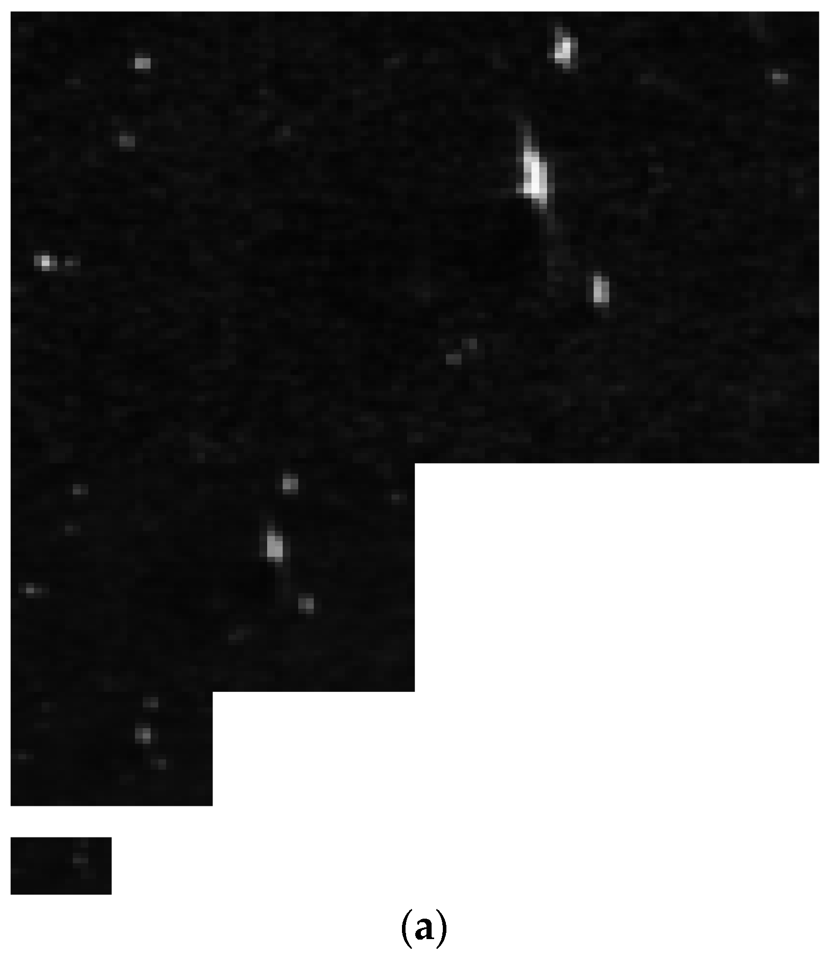
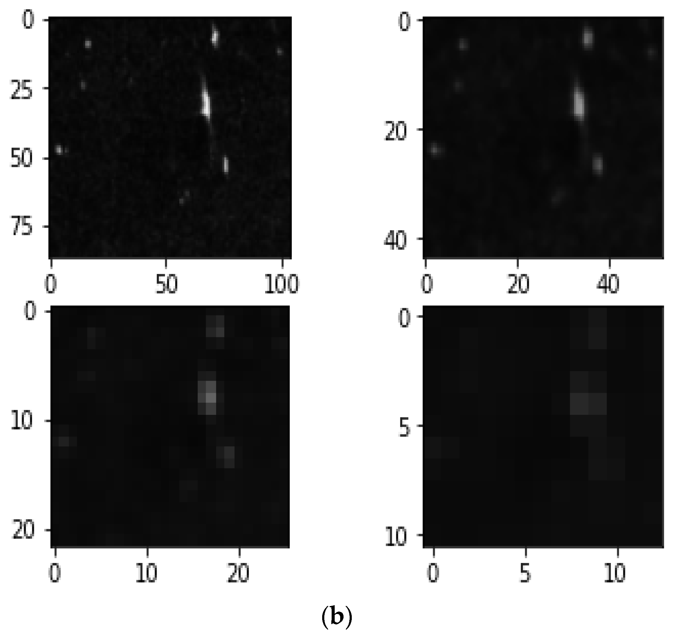
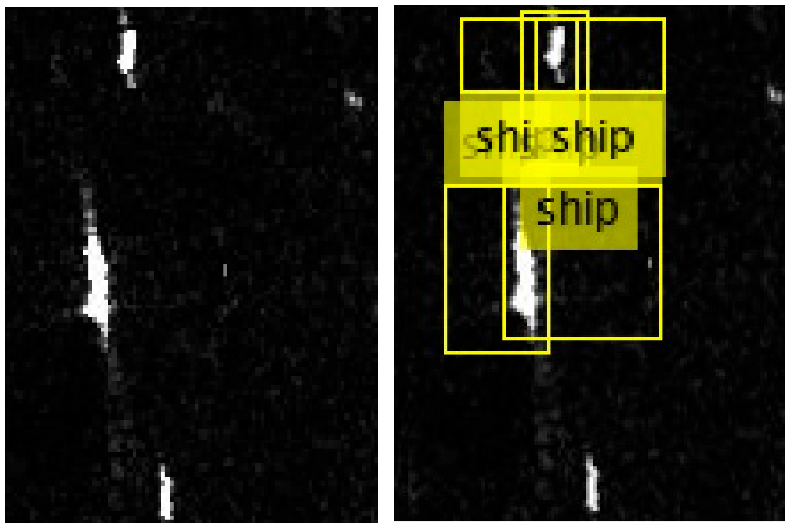
The output of this 3 × 3 convolution layer is the final extracted feature that can be given to the object detector. If we take as a set of the production of the bottom-up pathway {B1, B2, B3, B4} and {T1, T2, T3, T4} as input to the top-down pathway, then {F1, F2, F3, F4} is a set of extracted features. The sample feature pyramid of a SAR image is given in Figure 1a,b, a top-down and bottom-up path.

3. Materials and Methods

Dataset: This work was carried out at SRM Institute of Science and Technology, Chennai, India. The implementation was carried out with MATLAB with the proposed ACF-FRCNN method and later compared the proposed method’s performance with existing methods for ship and iceberg detection and classification. The SAR dataset was collected, and it had images of a ship and iceberg with a resolution of 75 × 75 pixel values, each image with two bands [3]. A total of 1604 images, of both ships and icebergs, were taken for validation and verification with training and testing. Among dataset sizes, 80% were trained, and 20% were tested.

Table 1. Accuracy comparison for ship detection over the SAR dataset with different methods.

Content	Description
Method used	ACF-FRCNN
Dataset	SAR images of ships and icebergs
Volume of dataset	1604
Implementation	MATLAB
Image resolution in pixels	75 × 75
Training dataset size	1283
Testing dataset size	321

describes the dataset information and implementation details of the detection of classification of icebergs and ships with the SAR dataset.

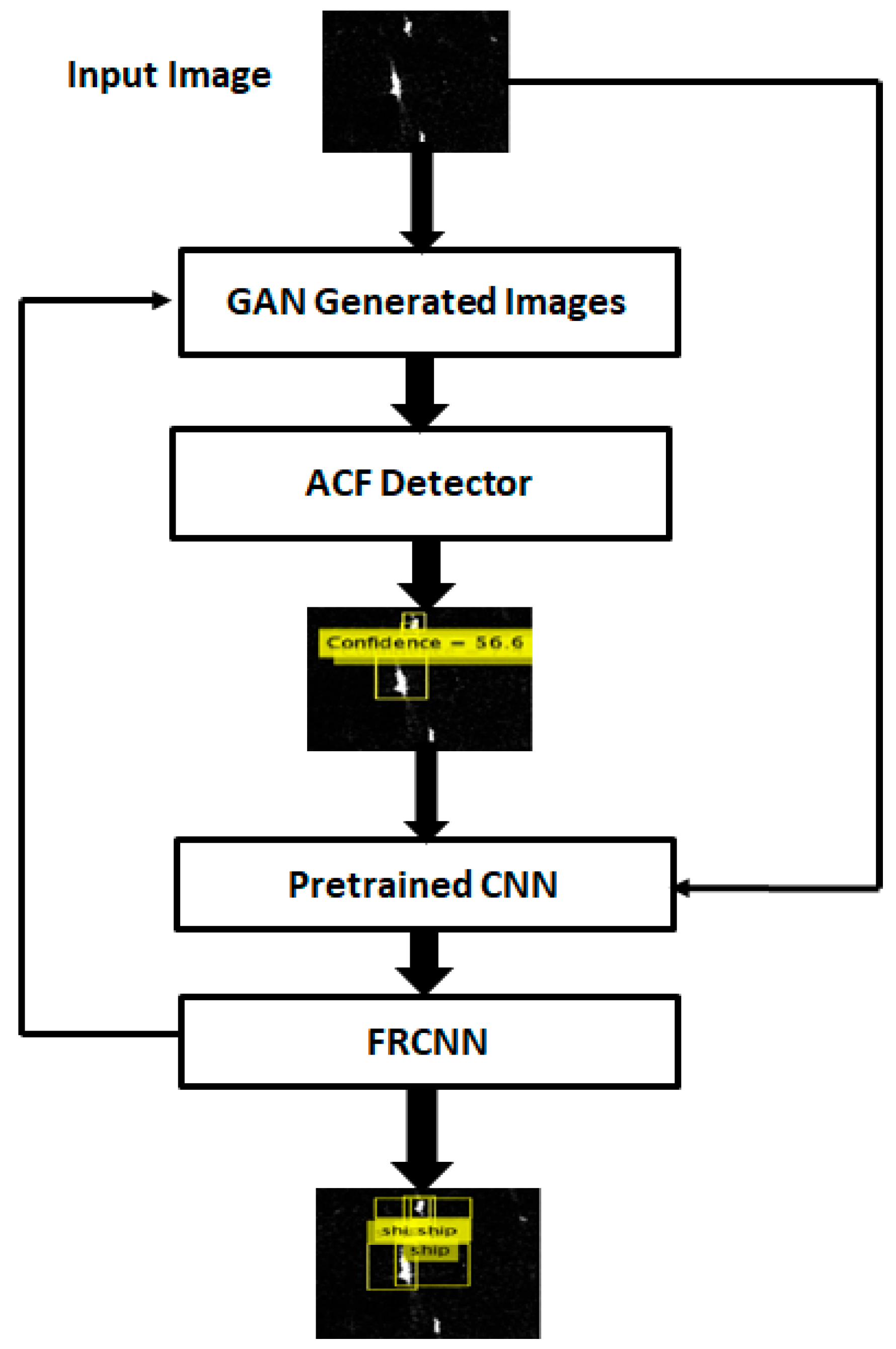
Recent trending methodologies such as GAN, ACF Detector, and FRCNN were used for better object detection performance in the proposed system. The first step of the proposed method is generating multi-transformed images of a single image using GAN architecture from the SAR image dataset [3]. The GAN architecture augments different images with another direction at a distant object location. Then, all generated images undergo an ACF detector to generate ROI in each image. Then, FRCNN generates a feature vector of all region proposals nominated by ACF, followed by object detection and object classification. The proposed research’s methods are explained in detail in the following segments.

3.1. GAN Architecture Training

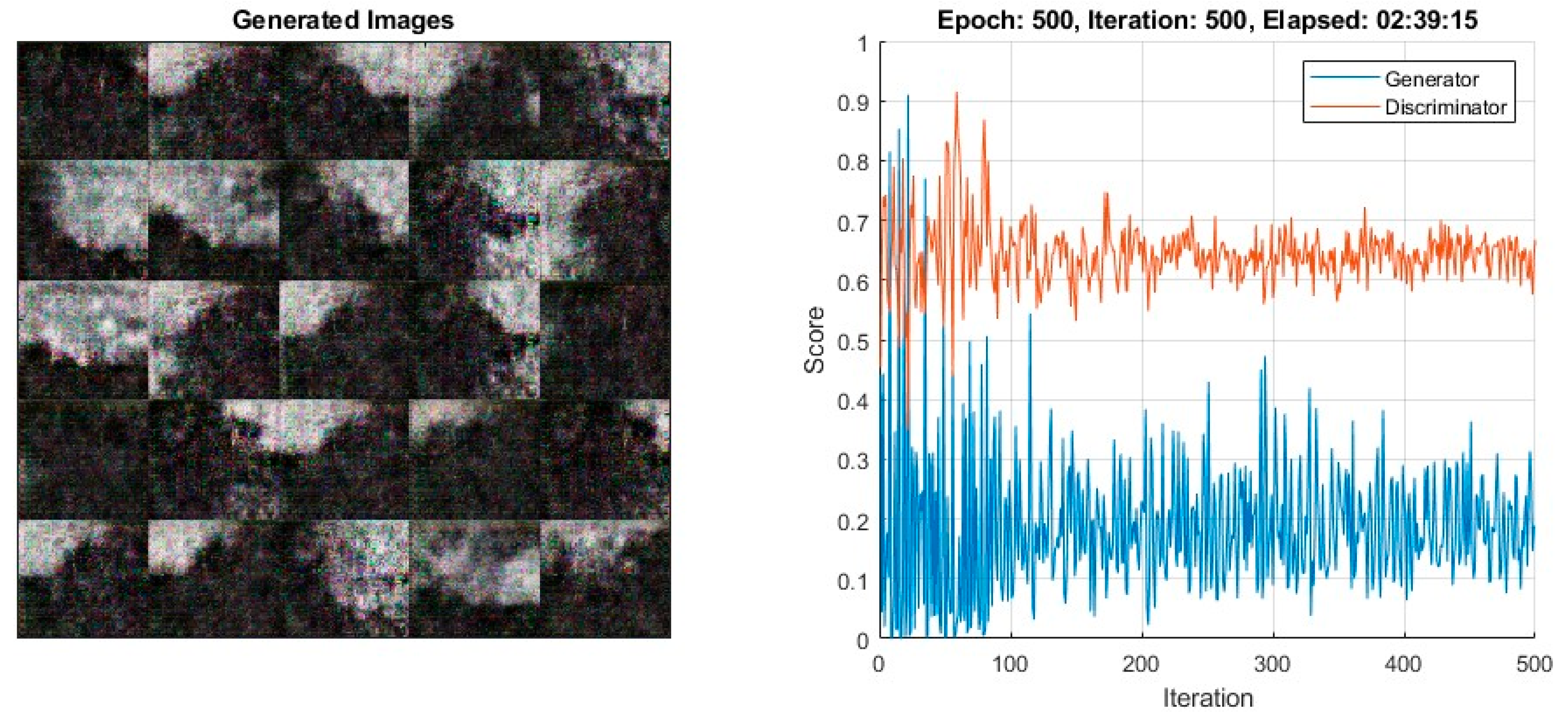
While performing a technical analysis in GAN, a winning model was discovered between the generator and discriminator. The generator tends to confuse the discriminator by producing data that look realistic but are not actually where the discriminator tries to distinguish images generated by generator and real ones. Both generator and discriminator have their loss function [2,3] for the initial process of dataset validation.

3.2. Loss Function of Generator

As mentioned earlier in the race of generator and discriminator, generator tries to confuse the discriminator by producing fake images. Let ȥ be a latent vector and g(ȥ) be data generated by the generator. Let d(g(ȥ)) be discriminator’s valuation of data generated by the generator. The loss function of the generator could be expressed as Equation (1).

$$\mathrm{LOSSg} = \mathrm{ERR}\left(\mathrm{d}\left(\mathrm{g}\left(ȥ\right)\right),1\right)$$

(1)

It is known that the model always tends to minimize the loss function. In this scenario, the generator also wants to minimize its loss function by reducing the difference between 1 and the discriminator valuation mark. There is a reason why the one is taken. Number 1 is given as a label for “true”.

3.3. Loss Function of Discriminator

The discriminator’s motive is to correctly identify the generated images of the generator as fake. Let d(r) be the valuation of the discriminator on accurate data. The loss function of the generator could be expressed as Equation (2).

$$\mathrm{LOSSd} = \mathrm{ERR}\left(\mathrm{d}\left(\mathrm{r}\right),1\right)+ \mathrm{ERR}\left(\mathrm{d}\left(\mathrm{g}\left(ȥ\right)\right),0\right)$$

(2)

Now take the generic loss function for binary classification, binary cross-entropy. Apply binary cross-entropy on the loss functions of the generator and discriminator. Express them, respectively, as Equations (3) and (4).

$$\mathrm{LOSSd} =-\sum \mathrm{r}\in \mathrm{R},ȥ\in \mathrm{Zlog}\left(\mathrm{d}\left(\mathrm{r}\right)\right)+ \log \left(1-\mathrm{d}\left(\mathrm{g}\left(ȥ\right)\right)\right)$$

(3)

$$\mathrm{LOSSg} =-\sum ȥ\in \mathrm{Zlog}(\mathrm{d}\left(\mathrm{g}\left(ȥ\right)\right)$$

(4)

The generator’s loss function will always be low because log (1) is zero. The next step is to optimize the model using loss functions. It is always better to train one model at a time. This model is suitable for considering the generator is fixed while training the discriminator, and the discriminator is set while training the generator.

3.4. Discriminator Training

Let the quantity of interest of the generator and discriminator be Qg and Qd. The value function in the amount of interest of the generator and discriminator is V(Qg Qd), expressed as Equation (5).

V(Qg Qd) = Er ﬥ pdata [log(d(r)) +Eȥ ﬥ pz log(1 − d(g(ȥ)))

(5)

Let y be g(ȥ); it is modified as Equations (6) and (7), respectively. The discriminator aims to maximize this value function.

$$\mathrm{V}\left(\mathrm{Qg} \mathrm{Qd}\right)= \mathrm{E}ř ﬥ \mathrm{pdata} \left[\log \left(\mathrm{d}\left(\mathrm{r}\right)\right)+\mathrm{E}ﬥ \mathrm{pz} \log \left(1-\mathrm{d}\left(\mathrm{y}\right)\right)\right]$$

(6)

$$\mathrm{V}\left(\mathrm{Qg} \mathrm{Qd}\right)=\int \mathrm{p} \mathrm{data} \left(\mathrm{x}\right)\left[\log \left(\mathrm{d}\left(\mathrm{r}\right)\right)+\mathrm{p} \mathrm{g}\left(\mathrm{x}\right) \log \left(1-\mathrm{d}\left(\mathrm{y}\right)\right)\right]$$

(7)

3.5. Generator Training

As discussed earlier, while training, the generator discriminator remains fixed, and the value function is calculated as for the discriminator and expressed as Equation (8). However, the difference is generator now tends to minimize this value function.

$$\mathrm{V}\left(\mathrm{Qg} \mathrm{Qd}\ast \right)= \mathrm{Er} ﬥ \mathrm{pdata} [\log \left(\mathrm{Qd}\ast \left(\mathrm{x}\right)\right)+\mathrm{E}ȥ ﬥ \mathrm{pz} \log \left(1-\left(\mathrm{Qd}\ast \left(\mathrm{x}\right)\right)\right)$$

(8)

3.6. ACF Model

The next step in iceberg and ship detection is obtaining regional proposals. The proposed system uses an aggregate channel feature detector as a region proposal extraction method. Before exploiting the influence of aggregated channel features in extracting region proposals, there is a need to have a vision of channels. Beyond generally known color channels, such as gray scale, RGB, hue saturation value (HSV), and LUV, two more channels are available: gradient magnitude and gradient histograms. The gradient of magnitude and histograms is known as the histogram of oriented gradient (HoG) features. In addition, with color channels, HoG channels also play a vital role in extracting features in the computer vision world. For extracting features, color information alone will not give better results because in the case of edge detection, with the use of a color channel, it can be identified whether there is a pixel in the edge, but it is incapable of recognizing the direction of edges. It is also a must to know information about the object’s movement. It can be possible with the help of HoG features.

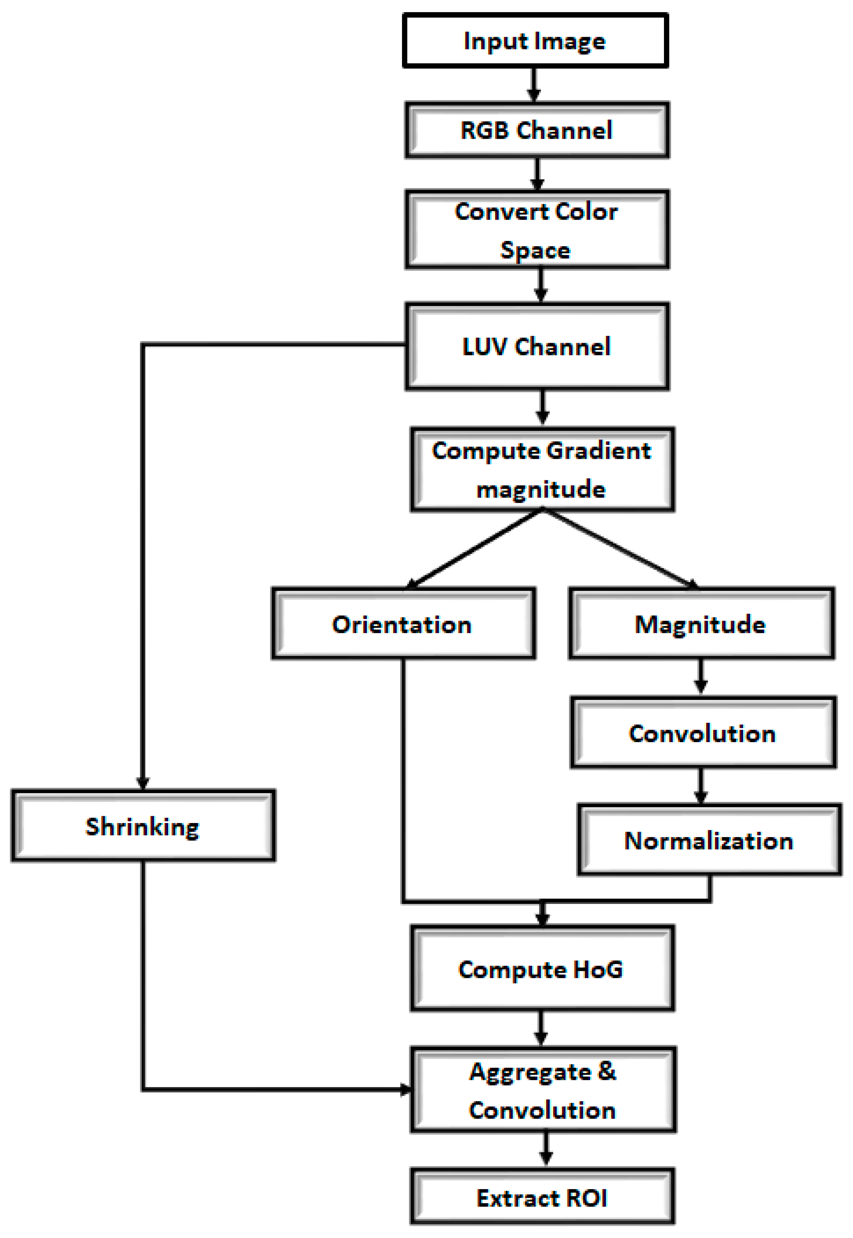
The idea in the proposed system is to aggregate all channels’ features using an ACF detector for region proposal extraction. If I is an input image, then H = Ω(I) is all channels of an image. After finding all channels, all blocks of pixels have to be summed up. As a result, features are single-pixel lookups in the aggregated channels. The role of ACF is set as RoI since ACF extracts ROI as the output of the ACF architecture model.

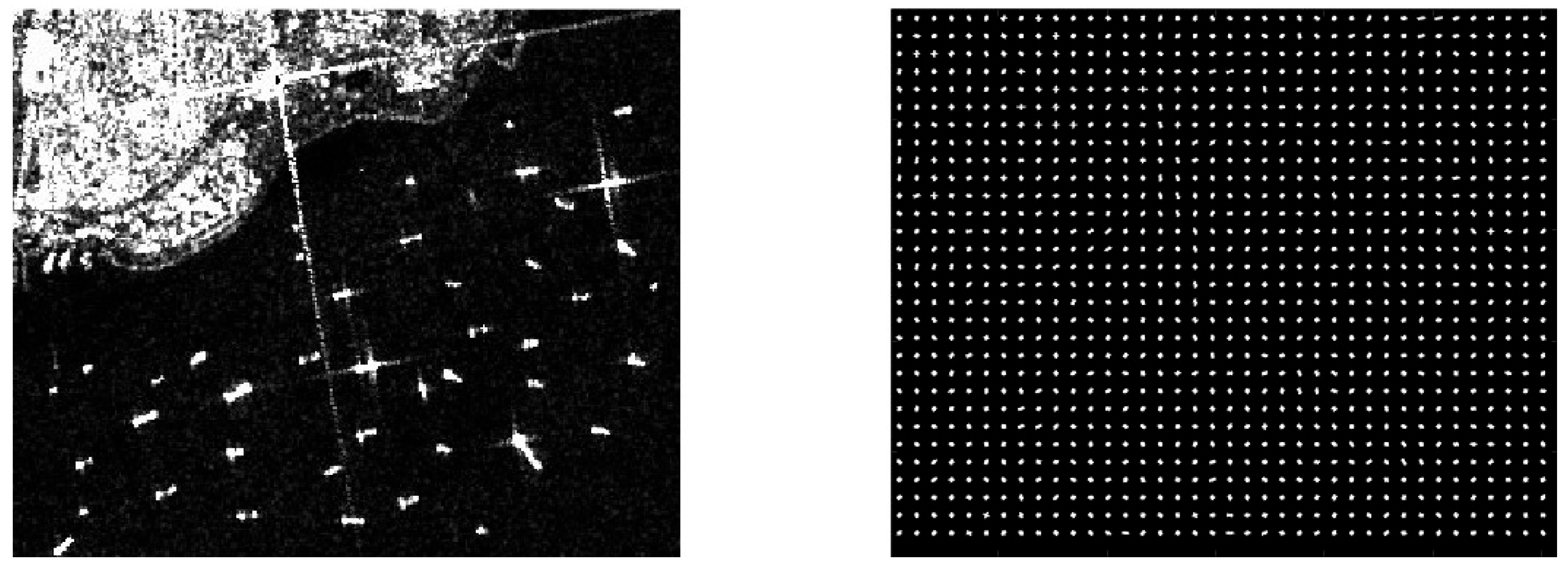
Thus, ACF gives fast feature pyramids with the set n number of layers, that is, Ƥ = { Ƥ1, Ƥ2, Ƥ3, Ƥ4, …… Ƥn,}. The proposed system used 3 LUV color channels, 6 HoG channels, and 1 normalized gradient channel. So a total of ten channels were used. The proposed ACF detector is shown in Figure 2. ACF can accelerate the model’s detection speed by extracting the right region proposal where the object could be present from the focus of a large SAR image. The extracted region proposals will be given as input to any detector. The proposed system uses FRCNN as an object detector network.

3.7. Object Detector—ResNet 50

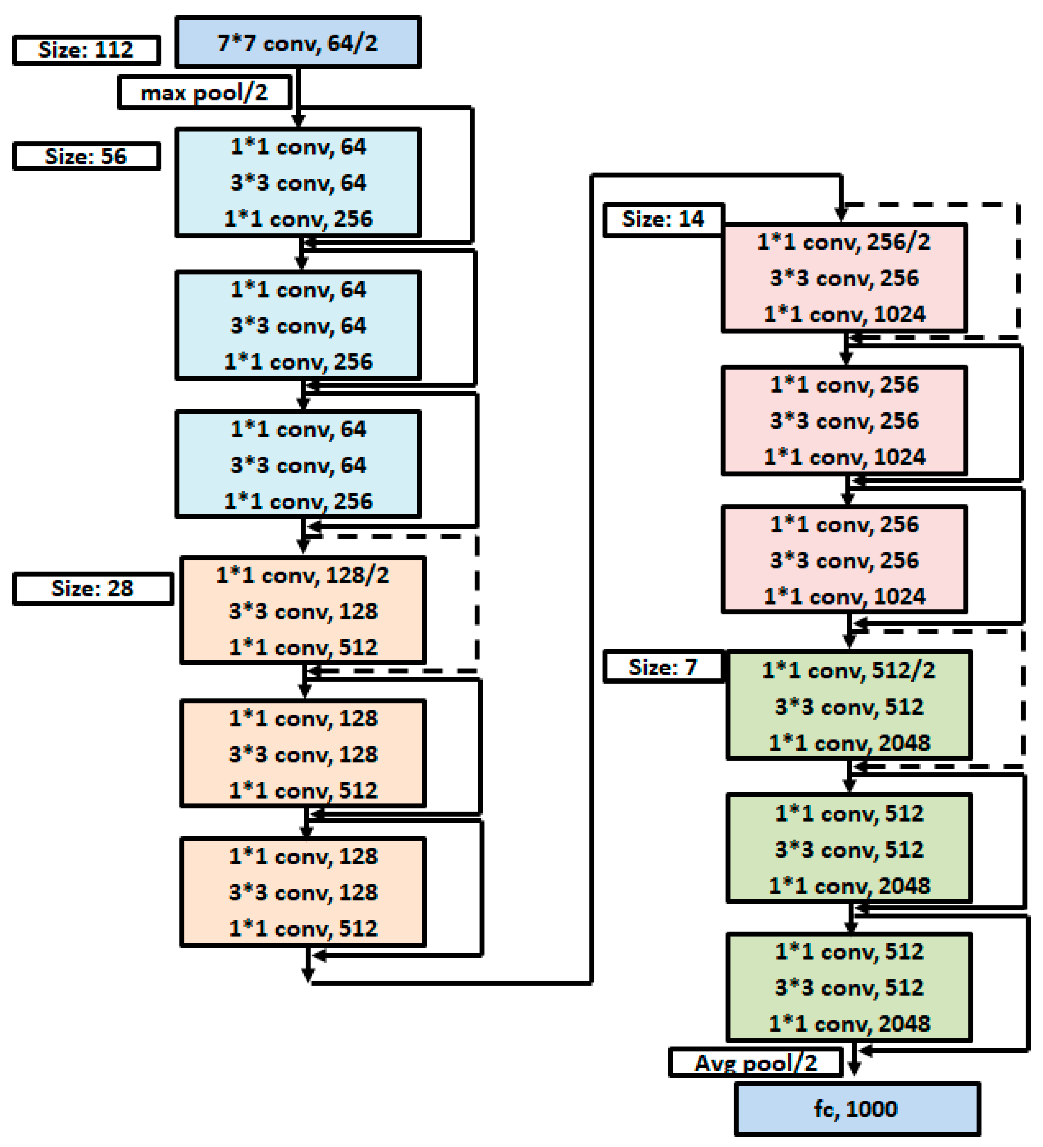
The ResNet 50 is a residual network deep with 50 layers. ResNet avoids the vanishing gradient problem, which occurs in classic CNN, by using skip connections. The architecture diagram of ResNet 50 is shown in Figure 3. Colour varies depending on output size.

3.8. The FRCNN Method

Region-based convolutional neural network is specifically designed for object detection. The most important focus of a region-based convolutional network is generating region proposals using selective search. The developed region proposals will be resized and converted into a feature vector. A typical CNN will treat these feature vectors where pre-trained SVM will be a classifier to classify the objects into specific classes. The R-CNN has some drawbacks such as heavy storage requirements, a rigid structure that could be more flexible for customization, and time complexity due to selective search. Due to these disadvantages, it is extended to the next level: FRCNN. Basic units of FRCNN are pre-trained CNN, ROI pooling layer, and two fully connected layers for Softmax layer and bounding box regression. The pre-trained convolutional neural network used in the proposed system is ResNet 50 which is explained in the last part of the work.

The proposed fast RCNN takes a full input image and proposals generated by ACF. Since our input image is a vast SAR image where the iceberg and ship are microscopic objects in an image whose shape and size are very complex to predict, ACF output is used as region proposals. The initial step of the proposed network is generating a feature map for the entire input image with the help of multiple convolutional layers and a max pooling layer. The next step is creating a feature vector for each proposal that ACF produces. This model can be applied by extracting features from the feature map for each proposal and then converting them into fixed-length feature vectors with the help of the ROI pooling layer.

With the help of the max pooling layer, the ROI pooling layer picks all features of the region proposal and converts it into a fixed-size vector, which could be in the size of height × width where height and width are hyperparameters. If the ROI window is in the size of height × width, then a grid of sub-windows can be created by dividing the ROI window into sub-window sizes. For example, if their m × n grid of sub-windows is there, each sub-window or cell size could be height/m × width/n. The third step is feeding these feature vectors to a set of fully connected layers, which ends with an output layer of two branches. The first branch is the softmax layer for predicting object classes: background, iceberg, and ship. Another branch has four values as a bounding box for locating predicted objects.

If there are k ROIs, the first branch calculates the discrete probability for all k numbers of ROI as P = {p0, p1, p2, p3,… pk,}. In the second branch bounding box, regression will be performed for calculating bb = {bbx, bby, bbw, bbh} where bbx is the x coordinate, bby is the y coordinate, bbw is the width, and bbh is the height of the bounding box. The bounding box will be created for all ROIs. For calculating loss for RCNN, two different losses, each for one branch, are used for weight updating. The first loss is for class prediction, which can be calculated as in Equations (9)–(11).

$$\mathrm{LOSSclass}\left(\mathrm{P},\mathrm{T}\right)=-\log \mathrm{PT}$$

(9)

where log is a loss for true class T, and the second loss is for bounding box regression, as expressed in Equation (10).

$$\mathrm{Lloc}\left(\mathrm{bbpred},\mathrm{T}\right)=\sum \mathrm{SMOOTHloc}\left(\mathrm{bbpredi}-\mathrm{Ti}\right)$$

(10)

where the notation “smoothloc” is represented as Equation (11).

$$\mathrm{SMOOTHloc} \left(\mathrm{x}\right)=\left\{\begin{array}{c}0.5x\ast x if \left|x\right|<1\\ \left|x\right|-0.5 otherwise\end{array}\right.$$

(11)

where bbpred is a predicted set of bounding boxes such as {bbpredx, bbpredy, bbpredw, bbpredh}; the proposed FRCNN architecture is given in Figure 4.

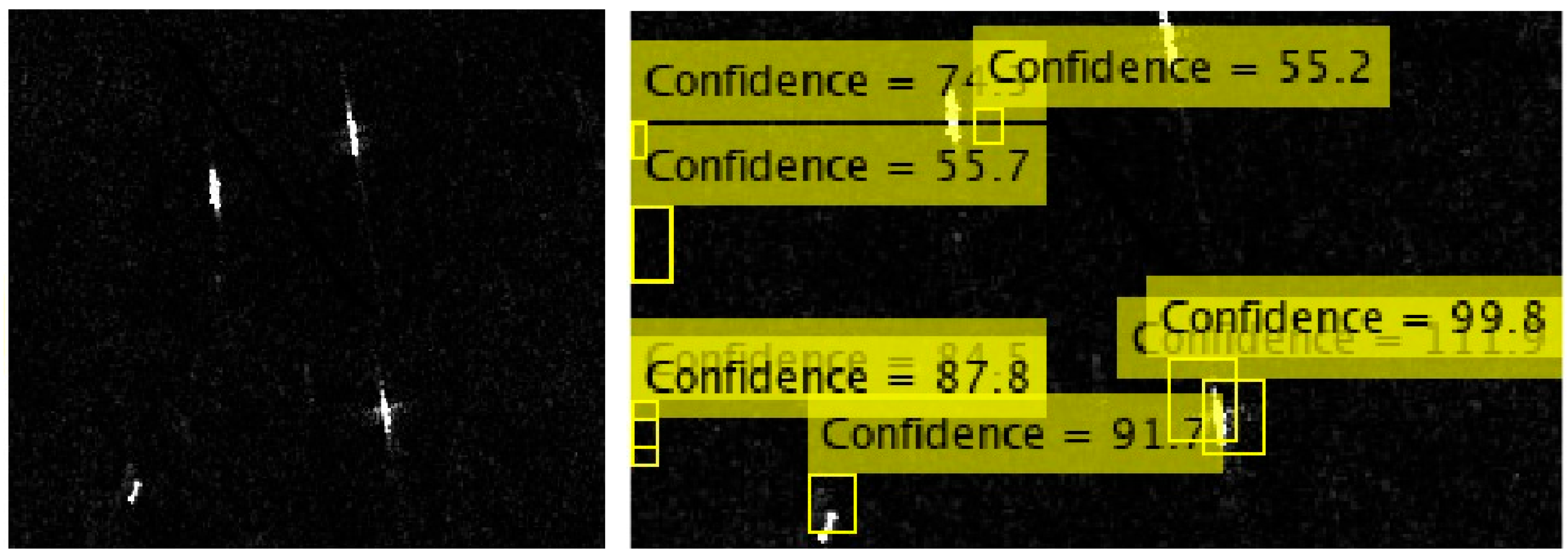
The algorithm of the proposed method FRCNN is structured below. It has procedure description, input, and output, and it is presented as Algorithm 1. Initially, the SAR input image is taken from the dataset and output such as class probability and bounding box set. Algorithm 1 procedure consists of computational functions such as RGB calculation of GAN and conversion of color space followed by LUV channel. The final LUV format image calculates magnitude and orientation. Then, the final image LUV is checked for ships or icebergs with a confidence score of region of proposal (ROP). This FRCNN must not be dropped to detect even small images, and the ROP confidence score is set at greater than 50% onwards with aggregate channel [21]. The next step of this FRCNN is to generate a feature map with ResNet with its appropriate layers. Next, the feature vectors are extracted for the image of LUV format with ROP of ACF, which underwent ResNet 50. Finally, it can find the probability and bounding box for inputting SAR images to detect ships and icebergs.

Algorithm 1: FRCNN method

Input: SAR Image I, Dataset Output: Class Probability, Bounding Box Procedure: For g = 1 to Ng where Ng is Number of image generated by GAN Calculate RGB channel for GAN[g] Convert RGB channel into Colors space Convert color space into LUV channel Calculate Magnitude and Orientation of LUV image of m x n     Mag(i,j) = √((∂GAN[g](i,j)/∂x)2 + (∂GAN[g](i,j)/∂y)2)                         Ori(i,j) = tan-1((∂GAN[g](i,j)/∂x)/(∂GAN[g](i,j)/∂x))                   Do Convolution of Magnitude Image                   Do Normalization of Convoluted Image         Compute HoG and Aggregate with LUV image         If (Confidence > 50) extract ROP from Aggregate channel // FRCNN working mechanism Generate Feature Map for Input Image I using RESNET convolutional and Maxpool layer Extract feature vector for each ROP of ACF Input fixed size vector to fully connected layers of RESNET 50 Calculate discrete probabilities of all region proposals P = {p0, p1, p2, p3,.. pk,}. bb= {bbx, bby, bbw, bbh} Calculate Lossclass (P, T) = -log PT which is log loss for true class T. Lloc (bbpred,T) = ∑ smoothloc (bbpredi-Ti) ${\mathrm{smooth}}_{\mathrm{loc}} \left(\mathrm{x}\right)=\left\{\begin{array}{c}0.5x\ast x if \left|x\right|<1\\ \left|x\right|-0.5 otherwise\end{array}\right. \mathrm{and}$ bbpred is predicted set of bounding box like {bbpredx, bbpredy, bbpredw, bbpredh End for For all ROI of I Ibb = {IbbxI, Ibby, Ibbw, Ibbh} where Ibb is bounding boxes of ROIs of Input image Pc = ∑ PPf-CNN/N where Pc is class probability of ROI of input image and PPf-CNN is output of fast CNN of all GAN images End for

The combination and usage of all the technologies in the proposed framework are explained in the architecture diagram and depicted in Figure 5.

4. Experimental Result

The proposed algorithm was implemented in MATLAB. The C-core dataset was used in the implementation [3]. The images of the ship and iceberg were stored as JSON files. These four fields are in a JSON file. The ID of the image, band one and band 2 data flattened as a numerical value, incidence angle, and the last filed refer to whether the given ROI is an iceberg. If the field contains 0, it shows it is a ship; if it has 1, it is an iceberg. The images in the dataset are in 75 × 75 sizes and have two bands. The expert team gives the labels. The implementation started with augmenting images by using GAN architecture. Figure 6, left side, demonstrates the sample output of augmented images. Figure 6 on the right side shows the training fashion and the generator and discriminator scores.

Then, the experiment was continued with an ACF detector where each augmented image color channel and histogram of the gradient had to be calculated. Figure 7 shows the sample output of the HoG of the SAR image.

After calculating the aggregation of all channels, the ACF detector finds the region proposal with the help of the confidence score. Figure 8 and Figure 9 show the output of the ACF detector. The inference was that a ship or iceberg was detected if the confidence score gained more than 50% as per the computation of Algorithm 1 with the guidance of ACF.

Then, fast R-CNN started with the region proposals of ACF detectors with the help of ResNet 50 backbone architecture. Finally, the bounding box located the object with classifications labels, whether an iceberg or a ship. Figure 9 shows an example of iceberg classification, and Figure 10 shows an example of ship classification.

5. Performance Analysis of Results

Table 2. Loss performance comparison for different methods for SAR dataset to detect ships and icebergs.

Method	Iter.1	Iter.2	Iter.3	Iter.4	Iter.5	Iter.6	Iter.7	Iter.8	Iter.9
ACF [17]	55.16	53.82	48.12	42.06	39.26	37.46	35.66	34.86	31.98
CNN [1]	79.23	76.29	73.65	70.13	61.43	52.54	43.31	34.23	32.12
FRCNN [8]	69.46	61.97	53.27	45.87	37.25	35.43	33.92	30.76	29.32
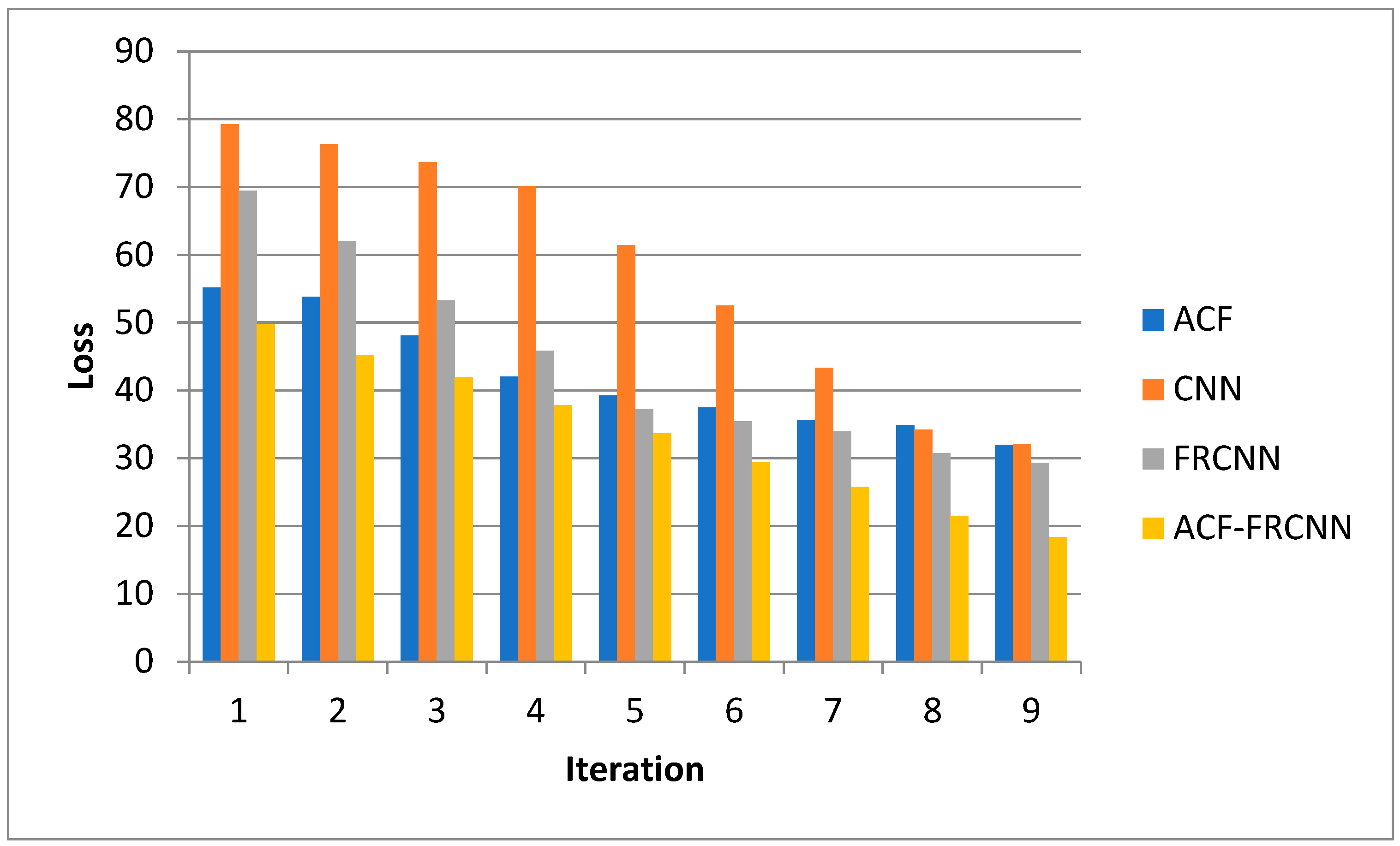
ACF-FRCNN	49.79	45.25	41.87	37.82	33.65	29.43	25.73	21.45	18.32

depicts the loss performance numerical illustration for four different methods: ACF, CNN, FRCNN, and ACF-FRCNN. This experimental loss performance was tested for the SAR dataset with an iterative method, and the number of data records was increased and tested with all methods as mentioned for the loss parameter. The inferences are that the loss gain is decreased for expanded records. The minimal loss for iteration 9 with 31.98%, 32.12%, 29.32%, and 18.32% was gained for ACF, CNN, FRCNN, and ACF-FRCNN. Among loss parameter performances, ACF-FRCNN had the best performance.

The proposed algorithm was compared for loss performance with CNN and ACF without fast RCNN and FRCNN without aggregate channel features. The analysis of loss is explained in the graph depicted in Figure 11.

Table 3. Accuracy comparison for ship detection over the SAR dataset with different methods.

Method	Iter.1	Iter.2	Iter.3	Iter.4	Iter.5	Iter.6	Iter.7	Iter.8
ACF [17]	44.21	50.29	56.92	62.34	68.78	74.97	80.63	86.12
CNN [1]	49.23	58.32	62.23	67.39	70.92	75.78	81.21	87.92
FRCNN [8]	56.12	59.76	67.13	69.32	74.89	76.54	85.72	89.14
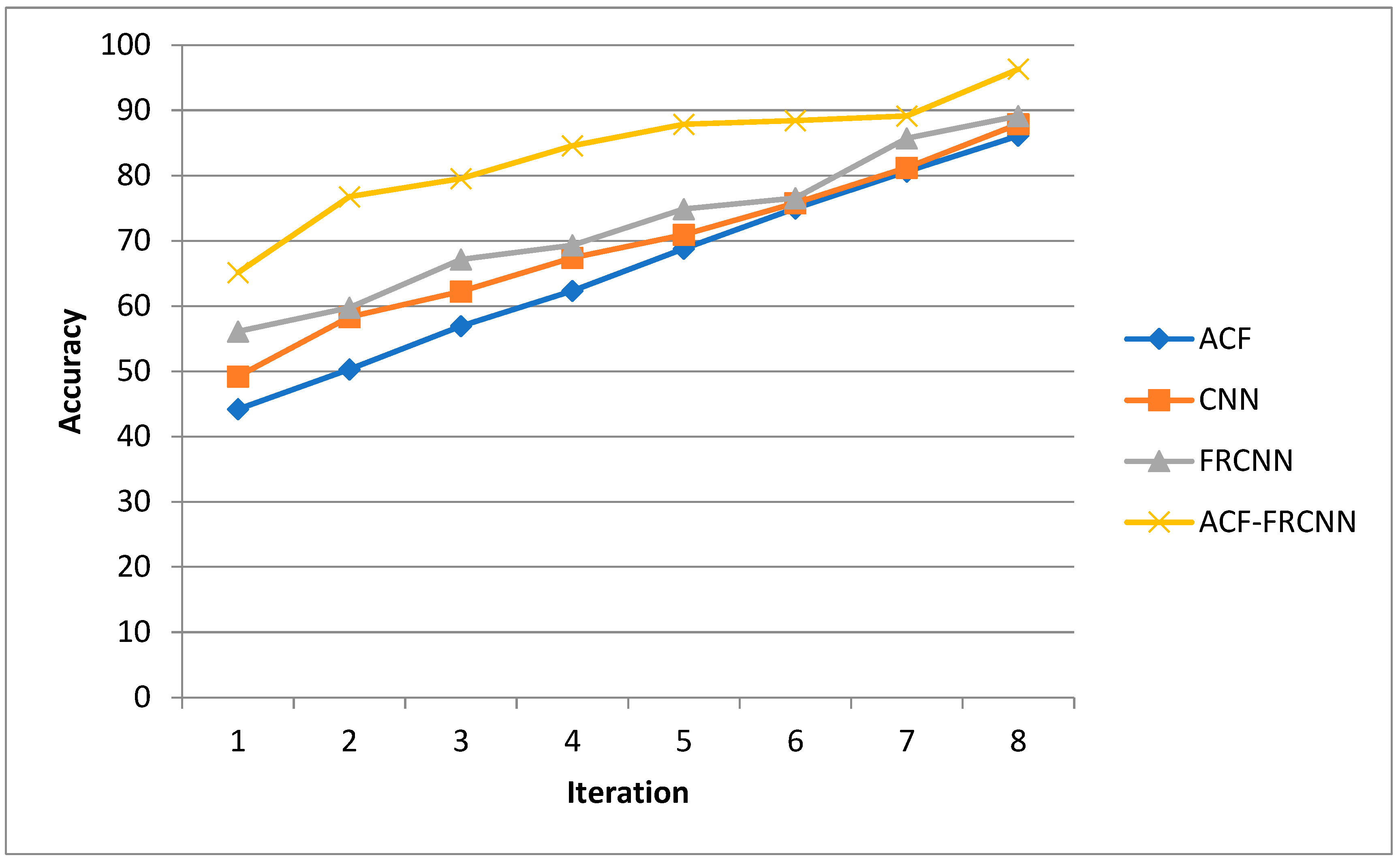
ACF-FRCNN	65.14	76.78	79.54	84.56	87.87	88.43	89.13	96.34

depicts the accuracy performance numerical illustration for four different methods ACF, CNN, FRCNN, and ACF-FRCNN. This experimental accuracy performance was tested for the SAR dataset with iteration, and the number of data records was increased and tested with all methods as mentioned for the accuracy parameter. The inference is that the accuracy gain is increased for records in the dataset. The maximum accuracy for iteration 8 with 86.12%, 87.92%, 89.14%, and 96.34% was achieved for ACF, CNN, FRCNN, and ACF-FRCNN, respectively. Among accuracy parameter performances, ACF-FRCNN had the best performance.

The proposed algorithm was compared for accuracy with CNN and ACF without FRCNN and FRCNN without ACF. The accuracy analysis is illustrated in the graph depicted in Figure 12.

The performance metrics for the proposed system are the F1 score, recall, and precision. Here, the metrics are calculated based on the is_iceberg attribute of the given JSON dataset file. The formula used to calculate precision, recall, and the F1 score is provided in Equations (12)–(14).

$$Precision=\frac{\mathrm{TP}}{\mathrm{TP}+\mathrm{FP}}$$

(12)

$$Recall=\frac{\mathrm{TP}}{\mathrm{TP}+\mathrm{FN}}$$

(13)

$$F1score=\frac{2\ast \left(\mathrm{Precision}\ast \mathrm{Recall}\right)}{\left(\mathrm{Precision}\ast \mathrm{Recall}\right)}$$

(14)

where TP is true positive, FP is false positive, and FN is false negative.

Table 4. Comparison of precision, recall, and F1 score performances for different methods.

Method	Precision	Recall	F1 Score
ACF [17]	84.76	83.76	84.26
CNN [1]	88.15	87.83	87.99
FRCNN [8]	94.65	95.32	94.98
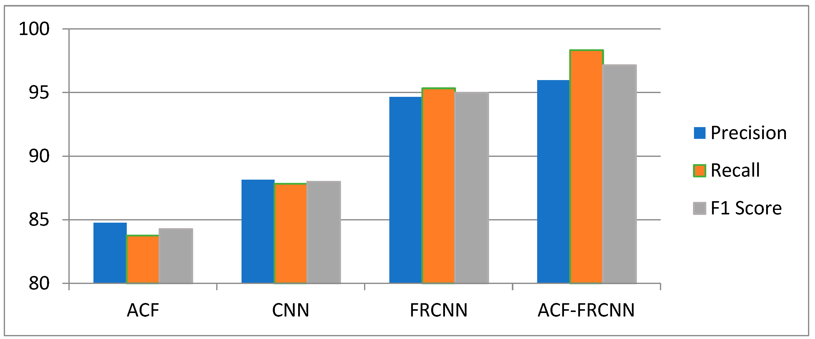
ACF-FRCNN	95.97	98.32	97.13

shows the F1 score, recall, and precision performances’ numerical illustration for four different methods: ACF, CNN, FRCNN, and ACF-FRCNN. This experimental F1 score, recall, and precision performance was tested for the SAR dataset. The number of data records was increased and tried with all of the methods mentioned: F1 score, recall, and precision parameters. The inference is that the F1 score, recall, and precision were increased when the number of records increased. The maximum F1 score, recall, and precision were 97.13%, 98.32%, and 95.97%, respectively, for the proposed ACF-FRCNN method. Among the F1 score, recall, and precision parameter performances of all four methods, ACF-FRCNN had the best performance.

F1 score is treated as a better evaluation metric than accuracy since it is a harmonic mean of precision and recall. The proposed method analysis is compared with other methods and shown in Figure 13.

6. Discussion and Comparison

The conducted experiment used MATLAB for ship and iceberg detection. The observation was made after inference with the proposed ACF-FRCNN algorithm. The performance parameters accuracy, recall, precision, and F1 score were measured and analyzed. These performance parameters were also compared with the ACF, CNN, and FRCNN methods. The dataset used 1604 SAR images with a pixel resolution of 75 × 75. From Figure 11 to Figure 13, it was observed that ACF combined with the FRCNN method outperformed 20% of the dataset in detecting ships and icebergs. The reason for including ACF with FRCNN was that FRCNN is only an RGB channel and is considered only a region proposal. However, ACF with FRCNN can measure the gradient magnitude and histogram. Thereby, the proposed ACF-FRCNN can detect ships and icebergs speedily and with high quality. Hence the novelty was achieved by combining ACF with the FRCNN algorithm for ship and iceberg detection and classification.

The previous methods were analyzed to state the proposed method’s performance. It was noticed that YOLO v3 gained an accuracy of 51.16% in detecting ship and iceberg discrimination [13]. The faster RCNN algorithm achieved accuracy for ship detection with 89.8% [32] with the SAR image dataset. The SSD introduced small ship detection accuracy of 92% and comparatively lesser accuracy than the proposed ACF-FRCNN method [33] over the SAR image dataset. Yet another CenterNet method achieved 83.71% accuracy for the SAR image dataset for detecting ships [34]. Work was introduced to detect ship detection, and it was a detection transformer (DETR) [35]. DETR achieved accuracy in detecting ships with a SAR dataset of 57.8%. After the detailed comparison, it was observed that ACF-FRCNN achieved higher performance.

Table 5. Various DL accuracy measure comparison with the proposed EDRL algorithm for ship and iceberg detection.

Used Method	Accuracy
YOLO v3 [13]	51.16%
Faster RCNN [32]	89.8%
SSD [33]	92%
CenterNet [34]	83.71%
DETR [35]	57.8%
Proposed ACF-FRCNN	96.34%

lists the accuracy performance value comparison of various methods, including the proposed ACF-FRCNN method.

The proposed ACF-FRCNN logic is a novelty since it produced optimal accuracy and faster detection of ships and icebergs over a SAR image dataset. It was also noticed that when the FRCNN was used to detect ships and icebergs directly, the FRCNN considered only color channels and missed some ROIs or added unwanted ROIs. However, when the proposed experiment initially fed ACF followed by FRCNN, the following outcome was introduced since ACF processed the region of the proposal with the variation of the gradient and the variation of the histograms. Thus, the outcome was optimum concerning accuracy, precision, etc., and detection speed was also increased. The YOLO method is often used for moving video frame applications such as traffic on roads, surveillance video systems, etc., for SAR image datasets, and the best effect to predict objects is the combined effect of the ACF and FRCNN methods, which is a novelty. In the future, the same proposed research work will be enhanced by using a high-resolution SAR image dataset, and we will also try to implement real-time automation for detecting ships and icebergs over the SAR image dataset.

7. Conclusions and Future Work

Small object detection in remote sensing images such as SAR images always plays a hectic role. For the past decade, various ML and DL algorithms have been applied to detect remotely sensed objects such as ships and icebergs. Even though some non-DL and DL-based algorithms are used to see ships and icebergs, performance measures still need improvement and efficiency. The proposed research reduces this complexity in detecting and classifying icebergs and ships with DL and non-DL combinations. The ACF detectors offer regions, and the FRCNN detector works on the proposals of ACF and produces accurate classification with a small amount of complexity. The proposed method achieved better numerical performance values: loss (18.32%), accuracy (96.34%), recall (98.32%), precision (95.97%), and the F1 score (97.13%). It was finally compared with other conventional methods, and it was claimed that the ACF and FRCNN methods outperformed and reduced the detector’s complexity. This framework can be extended with advanced pre-trained CNN and object detectors to include additional classes such as marine life. In the future, this proposed ACF and FRCNN algorithm will be developed with reinforcement concepts to train and automate remote sensing SAR-image-based submerged human body detection.