
Exploration and Comparison of the Effect of Conventional and Advanced Modeling Algorithms on Landslide Susceptibility Prediction: A Case Study from Yadong Country, Tibet

Abstract
1. Introduction
2. Materials
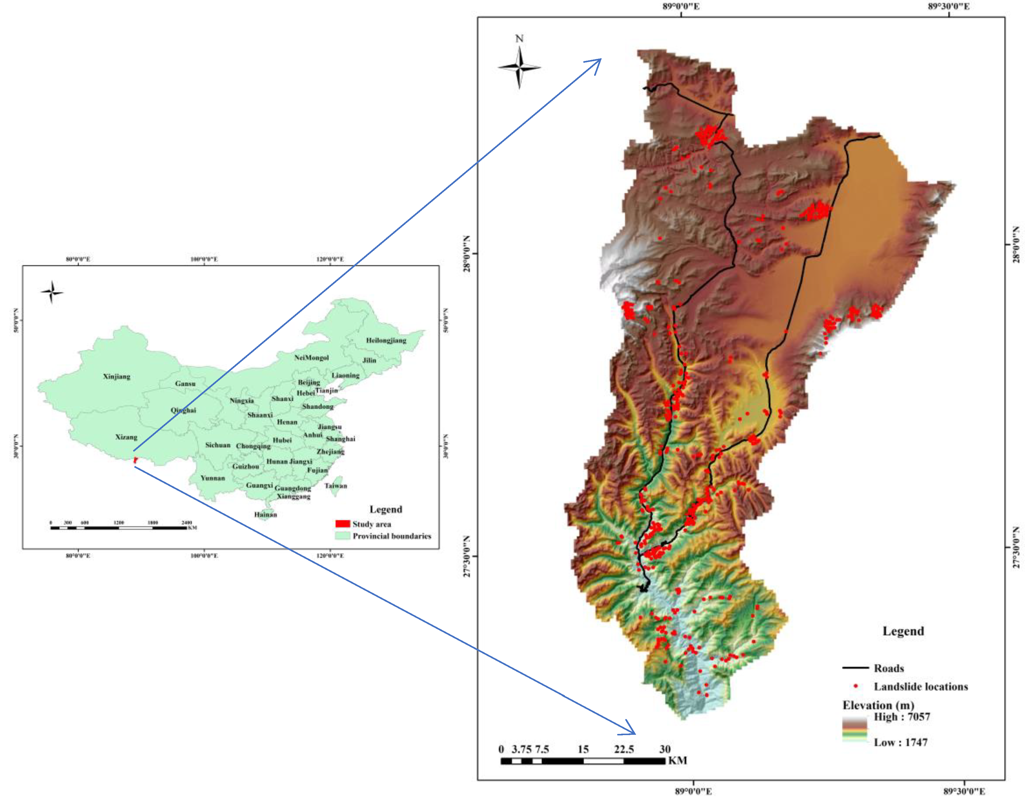
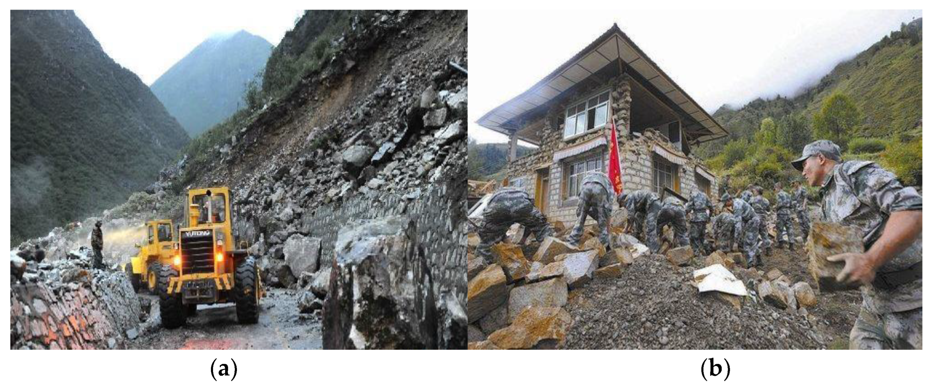
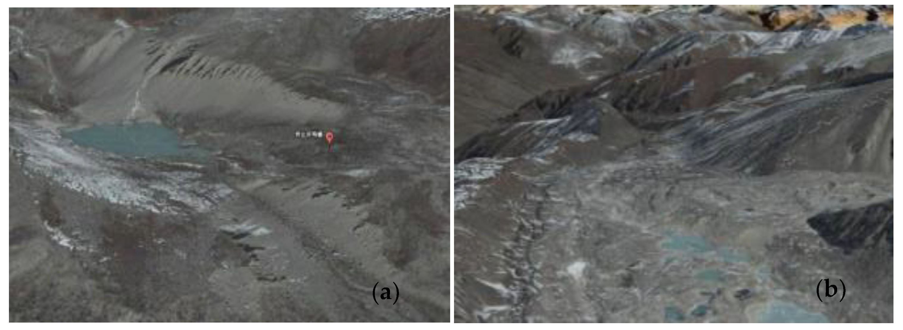
2.1. Study Area
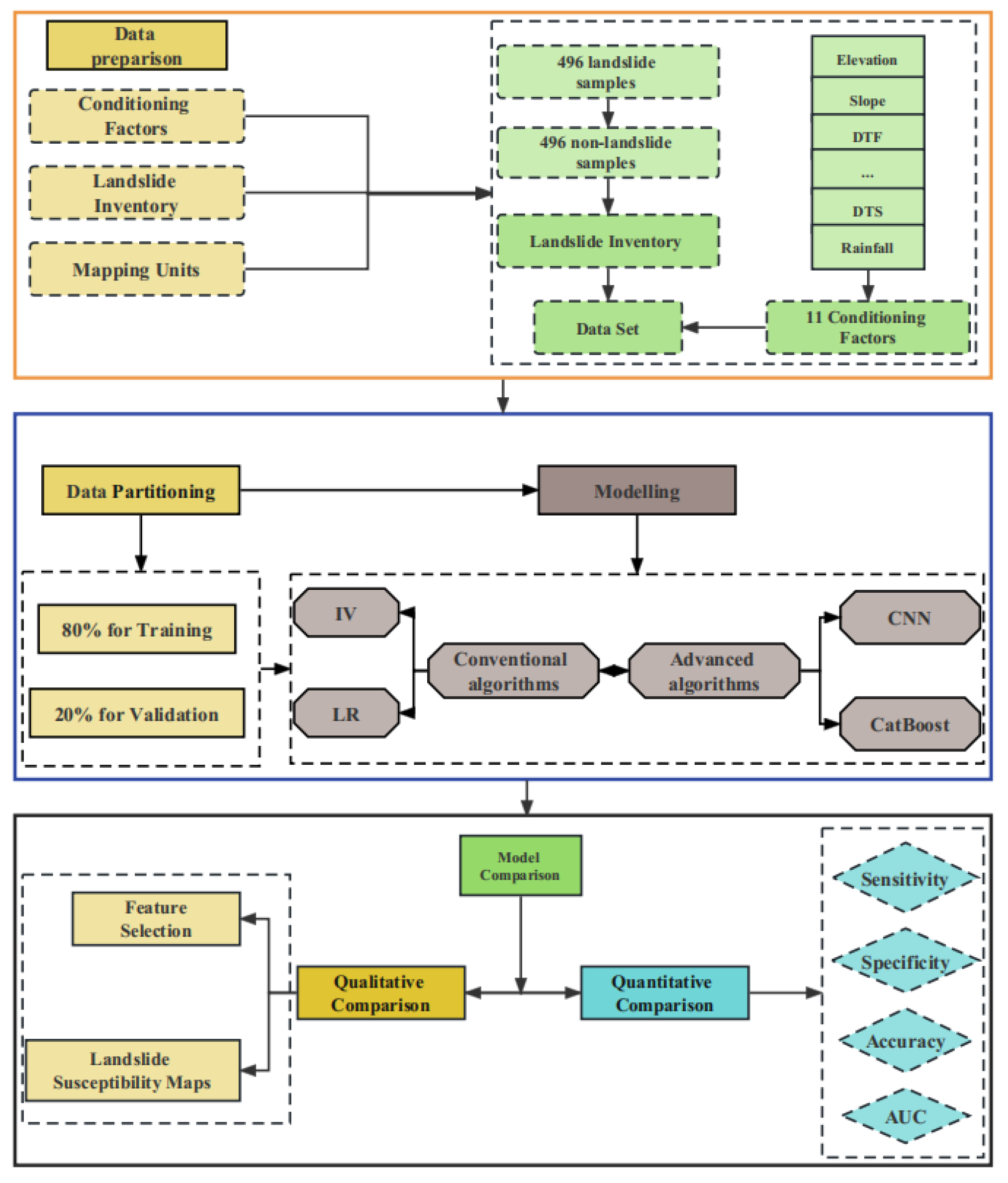
2.2. Data Preparation
2.2.1. Landslide Inventory
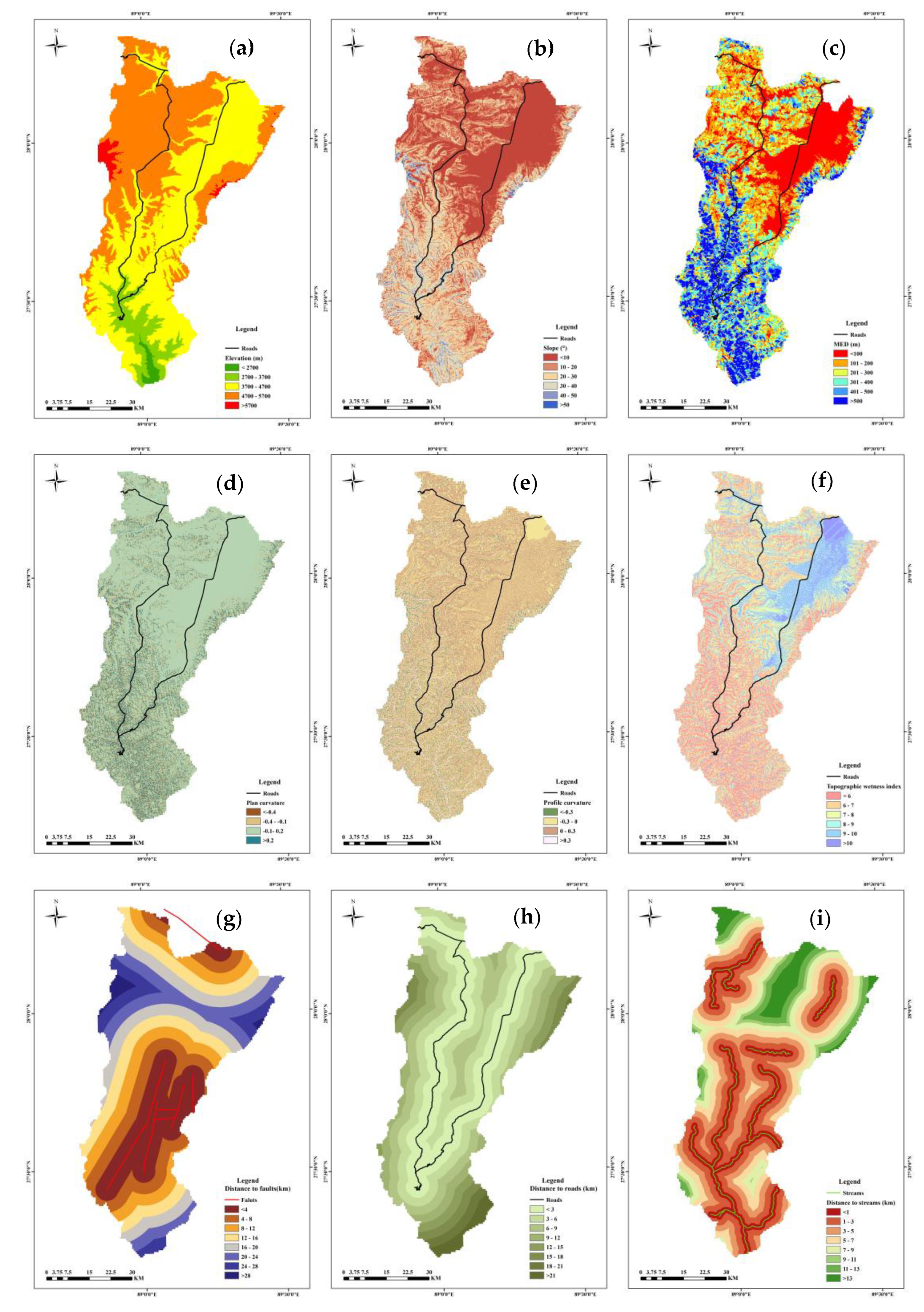
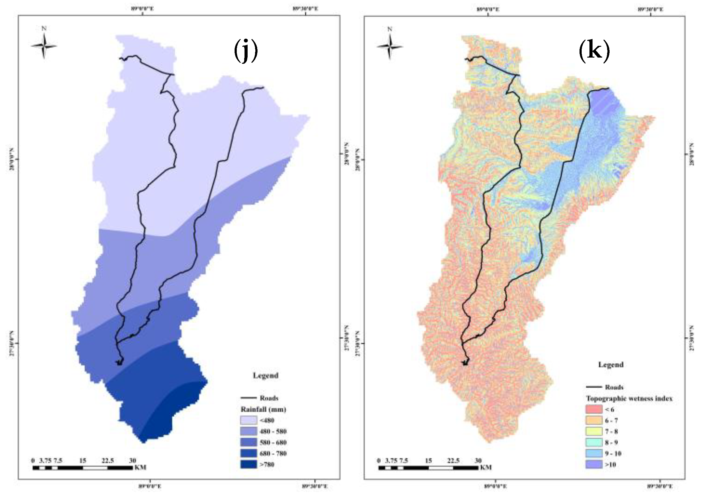
2.2.2. Conditioning Factors
2.2.3. Mapping Units
3. Methods
3.1. IV
3.2. LR
3.3. CatBoost
3.4. CNN
3.5. Models Evaluation
4. Results
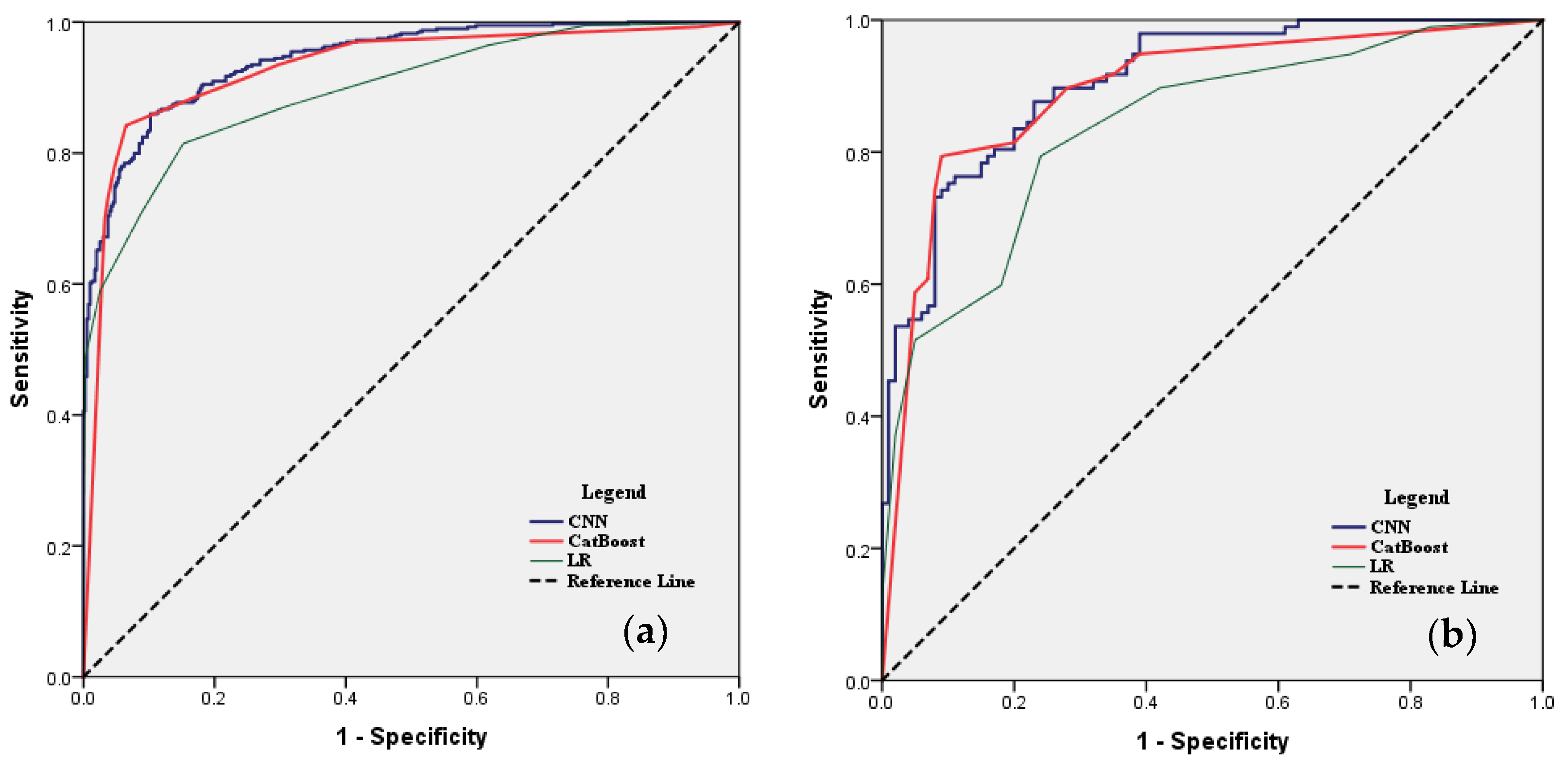
4.1. Performance and Comparison of Conventional and Advanced Algorithms
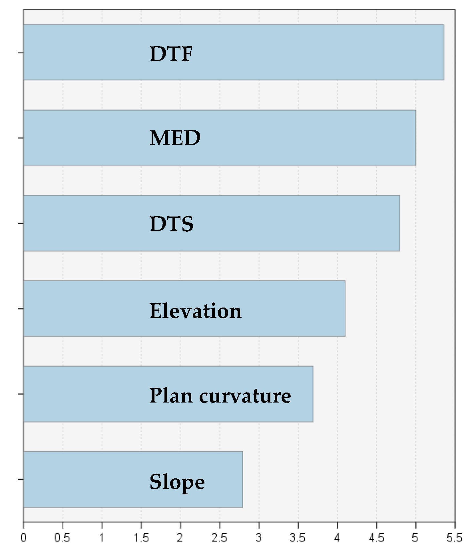
4.2. Evaluation of Conditioning Factors
4.2.1. Application of Conventional Algorithms
4.2.2. Application of Advanced Algorithms
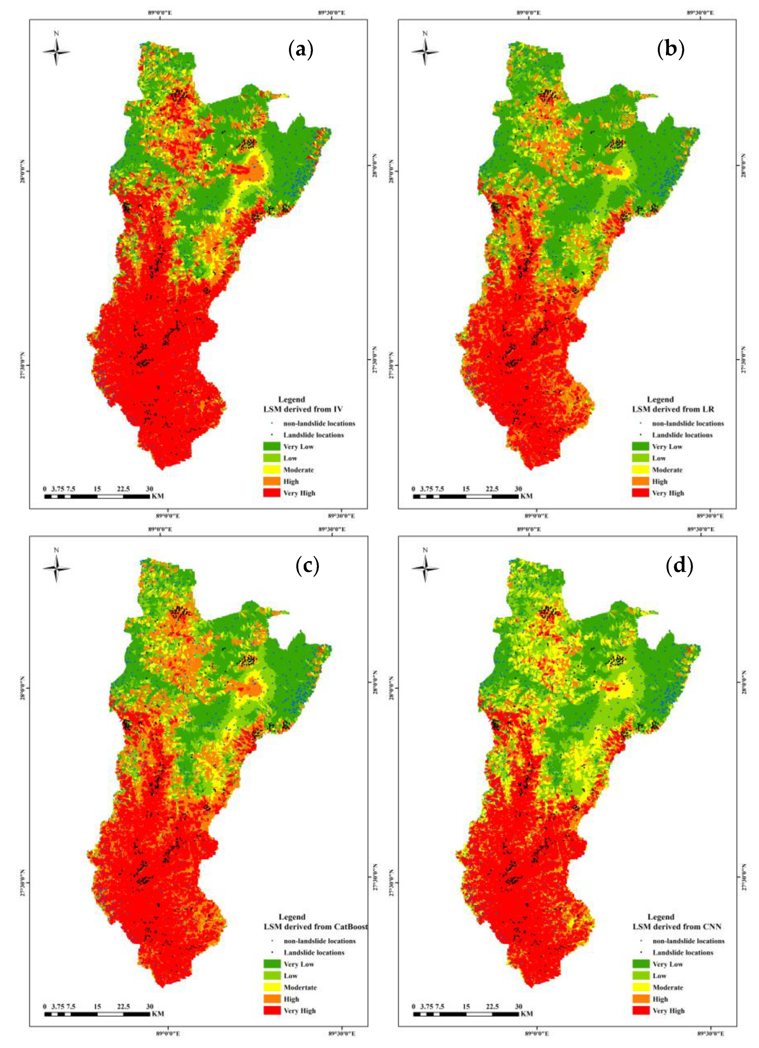
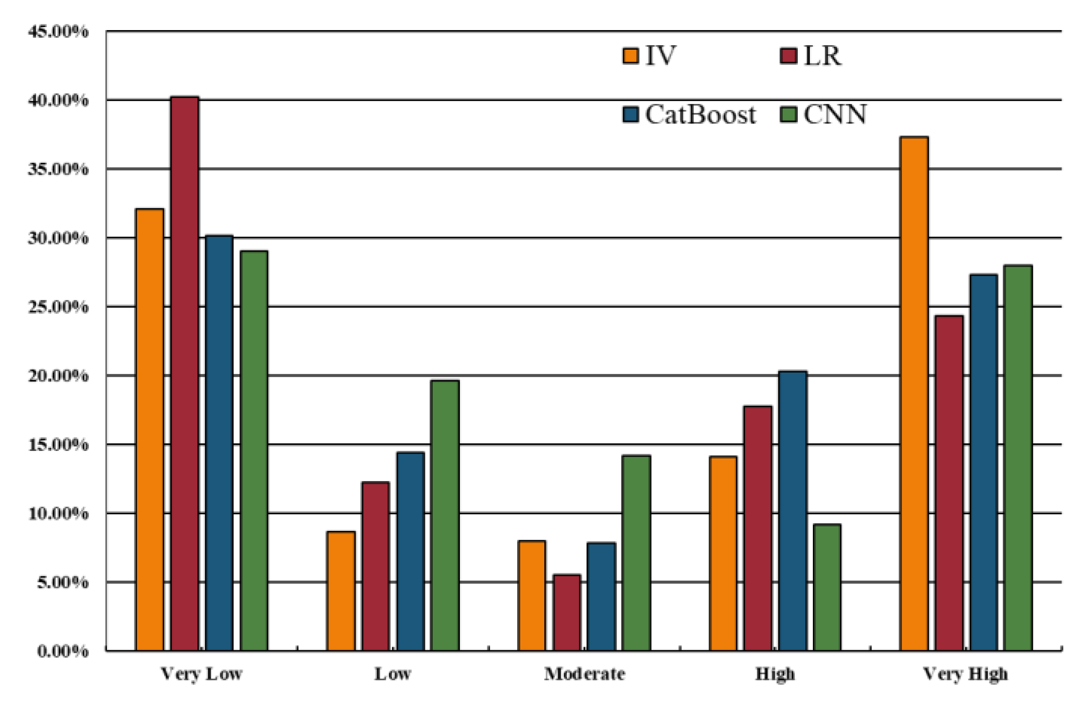
4.3. Landslide Susceptibility Mapping Results
5. Discussion
6. Conclusions
- There was a certain gap between the models. Compared to conventional algorithms, advanced algorithms performed better in terms of prediction accuracy and CNN performed the best in generalization, thus it is regarded as the best model in this study.
- The landslide susceptibility map predicted by CNN was more reasonable and the very high susceptibility areas were mainly distributed along the Yarlung Zangbo River.
- As for feature selection, IV and LR performed a more detailed analysis of conditioning factors, but the results were uncertain. The result analyzed by GI may be more reliable but fluctuates with the amount of data.
- The conventional algorithms are inferior to the advanced algorithms in accuracy and feature selection, but conventional algorithms have better resolvability and operability.
- There are possibilities for the combination of conventional and advanced algorithms, and further exploration is needed to improve prediction accuracy obviously.
- Models need to be validated more reliably.
Author Contributions
Funding
Institutional Review Board Statement
Informed Consent Statement
Data Availability Statement
Conflicts of Interest
References
- Das, I.; Sahoo, S.; van Westen, C.; Stein, A.; Hack, R. Landslide susceptibility assessment using logistic regression and its comparison with a rock mass classification system, along a road section in the northern Himalayas (India). Geomorphology 2010, 114, 627–637. [Google Scholar] [CrossRef]
- Achour, Y.; Boumezbeur, A.; Hadji, R.; Chouabbi, A.; Cavaleiro, V.; Bendaoud, E.A. Landslide susceptibility mapping using analytic hierarchy process and information value methods along a highway road section in Constantine, Algeria. Arab. J. Geosci. 2017, 10, 194. [Google Scholar] [CrossRef]
- Arabameri, A.; Pradhan, B.; Rezaei, K.; Lee, S.; Sohrabi, M. An ensemble model for landslide susceptibility mapping in a forested area. Geocarto Int. 2020, 35, 1680–1705. [Google Scholar] [CrossRef]
- Ni, H.Y.; Zheng, W.M.; Li, Z.L.; Ba, R.J. Recent catastrophic debris flows in Luding county, SW China: Geological hazards, rainfall analysis and dynamic characteristics. Nat. Hazards 2016, 55, 523–542. [Google Scholar] [CrossRef]
- Tong, L.; Qi, W.; An, G.; Liu, C. Remote sensing survey of major geological disasters in the Himalayas. J. Eng. Geol. 2019, 27, 496. [Google Scholar]
- Rai, P.K.; Mohan, K.; Kumra, V.K. Landslide hazard and its mapping using remote sensing and GIS. J. Sci. Res. 2014, 58, 1–13. [Google Scholar]
- Zhang, Q.; Liang, Z.; Liu, W.; Peng, W.; Huang, H.; Zhang, S.; Chen, L.; Jiang, K.; Liu, L. Landslide Susceptibility Prediction: Improving the Quality of Landslide Samples by Isolation Forests. Sustainability 2022, 14, 16692. [Google Scholar] [CrossRef]
- Corominas, J.; van Westen, C.; Frattini, P.; Cascini, L.; Malet, J.-P.; Fotopoulou, S.; Catani, F.; Van Den Eeckhaut, M.; Mavrouli, O.; Agliardi, F.; et al. Recommendations for the quantitative analysis of landslide risk. Bull. Eng. Geol. Environ. 2014, 73, 209–263. [Google Scholar] [CrossRef]
- Reichenbach, P.; Rossi, M.; Malamud, B.D.; Mihir, M.; Guzzetti, F. A Review of Statistically-Based Landslide Susceptibility Models. Earth Sci. Rev. 2018, 180, 60–91. [Google Scholar] [CrossRef]
- Shortliffe, E.H.; Buchanan, B.G. A model of inexact reasoning in medicine. Math. Biosci. 1975, 23, 351–379. [Google Scholar] [CrossRef]
- Korup, O.; Stolle, A. Landslide prediction from machine learning. Geol. Today 2014, 30, 26–33. [Google Scholar] [CrossRef]
- Chang, K.-T.; Merghadi, A.; Yunus, A.P.; Pham, B.T.; Dou, J. Evaluating scale effects of topographic variables in landslide susceptibility models using GIS-based machine learning techniques. Sci. Rep. 2019, 9, 12296. [Google Scholar] [CrossRef]
- Liang, Z.; Wang, C.; Zhang, Z.-M.; Khan, K.-U.-J. A comparison of statistical and machine learning methods for debris flow susceptibility mapping. Stoch. Environ. Res. Risk Assess. 2020, 34, 1887–1907. [Google Scholar] [CrossRef]
- Ghorbanzadeh, O.; Blaschke, T.; Gholamnia, K.; Meena, S.R.; Tiede, D.; Aryal, J. Evaluation of different machine learning methods and deep-learning convolutional neural networks for landslide detection. Remote Sens. 2019, 11, 196. [Google Scholar] [CrossRef]
- Liang, Z.; Wang, C.; Khan, K.U.J. Application and comparison of different ensemble learning machines combining with a novel sampling strategy for shallow landslide susceptibility mapping. Stoch. Environ. Res. Risk Assess. 2021, 35, 1243–1256. [Google Scholar] [CrossRef]
- Merghadi, A.; Yunus, A.P.; Dou, J.; Whiteley, J.; ThaiPham, B.; Bui, D.T.; Avtar, R.; Abderrahmane, B. Machine learning methods for landslide susceptibility studies: A comparative overview of algorithm performance. Earth Sci. Rev. 2020, 207, 103225. [Google Scholar] [CrossRef]
- Youssef, A.M. Landslide susceptibility delineation in the Ar-Rayth area, Jizan, Kingdom of Saudi Arabia, using analytical hierarchy process, frequency ratio, and logistic regression models. Environ. Earth Sci. 2015, 73, 8499–8518. [Google Scholar] [CrossRef]
- Li, L.; Lan, H.; Guo, C.; Zhang, Y.; Li, Q.; Wu, Y. A modified frequency ratio method for landslide susceptibility assessment. Landslides 2017, 14, 727–741. [Google Scholar] [CrossRef]
- Chen, Z.; Liang, S.; Ke, Y.; Yang, Z.; Zhao, H. Landslide susceptibility assessment using evidential belief function, certainty factor and frequency ratio model at Baxie River basin, NW China. Geocarto Int. 2019, 34, 348–367. [Google Scholar] [CrossRef]
- Gu, J.; Wang, Z.; Kuen, J.; Ma, L.; Shahroudy, A.; Shuai, B.; Liu, T.; Wang, X.; Wang, G.; Cai, J.; et al. Recent Advances in Convolutional Neural Networks. Pattern Recognit. 2018, 77, 354–377. [Google Scholar] [CrossRef]
- Ji, S.; Yu, D.; Shen, C.; Li, W.; Xu, Q. Landslide detection from an open satellite imagery and digital elevation model dataset using attention boosted convolutional neural networks. Landslides 2020, 17, 1337–1352. [Google Scholar] [CrossRef]
- Park, Y.; Yang, H.S. Convolutional neural network based on an extreme learning machine for image classification. Neurocomputing 2019, 339, 66–76. [Google Scholar] [CrossRef]
- Sameen, M.I.; Pradhan, B.; Lee, S. Application of convolutional neural networks featuring Bayesian optimization for landslide susceptibility assessment. Catena 2020, 186, 104249. [Google Scholar] [CrossRef]
- Fang, Z.; Wang, Y.; Peng, L.; Hong, H. Integration of convolutional neural network and conventional machine learning classifiers for landslide susceptibility mapping. Comput. Geosci. 2020, 139, 104470. [Google Scholar] [CrossRef]
- Varnes, D.J. Landslide Hazard Zonation: A Review of Principles and Practice; United Nations: New York, NY, USA, 1984.
- Kornejady, A.; Ownegh, M.; Bahremand, A. Landslide susceptibility assessment using maximum entropy model with two different data sampling methods. Catena 2017, 152, 144–162. [Google Scholar] [CrossRef]
- Van Westen, C.J.; Castellanos, E.; Kuriakose, S.L. Spatial data for landslide susceptibility, hazard, and vulnerability assessment: An overview. Eng. Geol. 2008, 102, 112–131. [Google Scholar] [CrossRef]
- Hong, H.; Pradhan, B.; Xu, C.; Bui, D.T. Spatial prediction of landslide hazard at the Yihuang area (China) using two-class kernel logistic regression, alternating decision tree and support vector machines. Catena 2015, 133, 266–281. [Google Scholar] [CrossRef]
- Sameen, M.I.; Pradhan, B.; Bui, D.T.; Alamri, A.M. Systematic sample subdividing strategy for training landslide susceptibility models. Catena 2019, 187, 104358. [Google Scholar] [CrossRef]
- Magliulo, P.; DiLisio, A.; Russo, F.; Zelano, A. Geomorphology and landslide susceptibility assessment using GIS and bivariate statistics: A case study in southern Italy. Nat. Hazards 2008, 47, 411–435. [Google Scholar] [CrossRef]
- Zevenbergen, L.W.; Thorne, C.R. Quantitative analysis of land surface topography. Earth Surf. Process. Landf. 1987, 12, 47–56. [Google Scholar] [CrossRef]
- Pradhan, B. Landslide susceptibility mapping of a catchment area using frequency ratio, fuzzy logic and multivariate logistic regression approaches. J. Indian Soc. Remote Sens. 2010, 38, 301–320. [Google Scholar] [CrossRef]
- Evans, I.S. An integrated system of terrain analysis and slope mapping. Z. Geomorphol. Suppl. Stuttg. 1980, 36, 274–295. [Google Scholar]
- Liang, Z.; Wang, C.; Duan, Z.; Liu, H.; Liu, X.; Jan Khan, K.U. A hybrid model consisting of supervised and unsupervised learning for landslide susceptibility mapping. Remote Sens. 2021, 13, 1464. [Google Scholar] [CrossRef]
- Carrara, A.; Cardinali, M.; Detti, R.; Guzzetti, F.; Pasqui, V.; Reichenbach, P. GIS techniques and statistical models in evaluating landslide hazard. Earth Surf. Process. Landf. 1991, 16, 427–445. [Google Scholar] [CrossRef]
- Carrara, A.; Cardinali, M.; Guzzetti, F.; Reichenbach, P. GIS technology in mapping landslide hazard. In Geographical Information Systems in Assessing Natural Hazards; Springer: Berlin/Heidelberg, Germany, 1995; pp. 135–175. [Google Scholar]
- Carrara, A.; Guzzetti, F. (Eds.) Geographical Information Systems in Assessing Natural Hazards; Springer Science & Business Media: Berlin/Heidelberg, Germany, 2013; Volume 5. [Google Scholar]
- Yin, K.L. Statistical prediction model for slope instability of metamorphosed rocks. In Proceedings of the 5th International Symposium on Landslides, Lausanne, Switzerland, 10–15 July 1988; Volume 2, pp. 1269–1272. [Google Scholar]
- Chen, W.; Yang, Z. Landslide susceptibility modeling using bivariate statistical-based logistic regression, naïve Bayes, and alternating decision tree models. Bull. Eng. Geol. Environ. 2023, 82, 190. [Google Scholar] [CrossRef]
- Ganga, A.; Elia, M.; D’Ambrosio, E.; Tripaldi, S.; Capra, G.F.; Gentile, F.; Sanesi, G. Assessing landslide susceptibility by coupling spatial data analysis and logistic model. Sustainability 2022, 14, 8426. [Google Scholar] [CrossRef]
- Ye, P.; Yu, B.; Chen, W.; Liu, K.; Ye, L. Rainfall-induced landslide susceptibility mapping using machine learning algorithms and comparison of their performance in Hilly area of Fujian Province, China. Nat. Hazards 2022, 113, 965–995. [Google Scholar] [CrossRef]
- Sahin, E.K. Comparative analysis of gradient boosting algorithms for landslide susceptibility mapping. Geocarto Int. 2022, 37, 2441–2465. [Google Scholar] [CrossRef]
- Krizhevsky, A.; Sutskever, I.; Hinton, G.E. ImageNet Classification with Deep Convolutional Neural Networks. Commun. ACM 2017, 60, 84–90. [Google Scholar] [CrossRef]
- Renza, D.; Cárdenas, E.A.; Martinez, E.; Weber, S.S. CNN-Based Model for Landslide Susceptibility Assessment from Multispectral Data. Appl. Sci. 2022, 12, 8483. [Google Scholar] [CrossRef]
- Saha, S.; Saha, A.; Hembram, T.K.; Mandal, K.; Sarkar, R.; Bhardwaj, D. Prediction of spatial landslide susceptibility applying the novel ensembles of CNN, GLM and random forest in the Indian Himalayan region. Stoch. Environ. Res. Risk Assess. 2022, 36, 3597–3616. [Google Scholar] [CrossRef]
- Liang, Z.; Liu, W.; Peng, W.; Chen, L.; Wang, C. Improved shallow landslide susceptibility prediction based on statistics and ensemble learning. Sustainability 2022, 14, 6110. [Google Scholar] [CrossRef]
- Lv, L.; Chen, T.; Dou, J.; Plaza, A. A hybrid ensemble-based deep-learning framework for landslide susceptibility mapping. Int. J. Appl. Earth Obs. Geoinf. 2022, 108, 102713. [Google Scholar] [CrossRef]
- Ling, X.; Zhu, Y.; Ming, D.; Chen, Y.; Zhang, L.; Du, T. Feature Engineering of Geohazard Susceptibility Analysis Based on the Random Forest Algorithm: Taking Tianshui City, Gansu Province, as an Example. Remote Sens. 2022, 14, 5658. [Google Scholar] [CrossRef]
- Huang, F.; Tao, S.; Chang, Z.; Huang, J.; Fan, X.; Jiang, S.-H.; Li, W. Efficient and automatic extraction of slope units based on multi-scale segmentation method for landslide assessments. Landslides 2021, 18, 3715–3731. [Google Scholar] [CrossRef]
- Chang, Z.; Catani, F.; Huang, F.; Liu, G.; Meena, S.R.; Huang, J.; Zhou, C. Landslide susceptibility prediction using slope unit-based machine learning models considering the heterogeneity of conditioning factors. J. Rock Mech. Geotech. Eng. 2023, 15, 1127–1143. [Google Scholar] [CrossRef]
- Huang, F.; Pan, L.; Fan, X.; Jiang, S.H.; Huang, J.; Zhou, C. The uncertainty of landslide susceptibility prediction modeling: Suitability of linear conditioning factors. Bull. Eng. Geol. Environ. 2022, 81, 182. [Google Scholar] [CrossRef]
- Bravo-López, E.; Del Castillo, T.F.; Sellers, C.; Delgado-García, J. Landslide susceptibility mapping of landslides with artificial neural networks: Multi-approach analysis of back propagation algorithm applying the neuralnet package in Cuenca, Ecuador. Remote Sens. 2022, 14, 3495. [Google Scholar] [CrossRef]
- Chen, W.; Li, Y. GIS-based evaluation of landslide susceptibility using hybrid computational intelligence models. Catena 2020, 195, 104777. [Google Scholar] [CrossRef]
- Dou, J.; Yunus, A.P.; Bui, D.T.; Merghadi, A.; Sahana, M.; Zhu, Z.; Chen, C.W.; Han, Z.; Pham, B.T. Improved landslide assessment using support vector machine with bagging, boosting, and stacking ensemble machine learning framework in a mountainous watershed, Japan. Landslides 2020, 17, 641–658. [Google Scholar] [CrossRef]
- Pourghasemi, H.R.; Kariminejad, N.; Amiri, M.; Edalat, M.; Zarafshar, M.; Blaschke, T.; Cerda, A. Assessing and mapping multi-hazard risk susceptibility using a machine learning technique. Sci. Rep. 2020, 10, 3203. [Google Scholar] [CrossRef]
- Murillo-García, F.G.; Steger, S.; Alcántara-Ayala, I. Landslide susceptibility: A statistically-based assessment on a depositional pyroclastic ramp. J. Mt. Sci. 2019, 16, 561–580. [Google Scholar] [CrossRef]
- Zhang, Y.-X.; Lan, H.-X.; Li, L.-P.; Wu, Y.-M.; Chen, J.-H.; Tian, N.-M. Optimizing the frequency ratio method for landslide susceptibility assessment: A case study of the Caiyuan Basin in the southeast mountainous area of China. J. Mt. Sci. 2020, 17, 340–357. [Google Scholar] [CrossRef]
- Saygin, F.; Şişman, Y.; Dengiz, O.; Şişman, A. Spatial assessment of landslide susceptibility mapping generated by fuzzy-AHP and decision tree approaches. Adv. Space Res. 2023, 71, 5218–5235. [Google Scholar] [CrossRef]
- Liang, Z.; Wang, C.; Han, S.; Khan, K.U.J.; Liu, Y. Classification and susceptibility assessment of debris flow based on a semiquantitative method combination of the fuzzy C-means algorithm, factor analysis and efficacy coefficient. Nat. Hazards Earth Syst. Sci. 2020, 20, 1287–1304. [Google Scholar] [CrossRef]
- Pourghasemi, H.R.; Moradi, H.R.; Fatemi Aghda, S.M. Landslide susceptibility mapping by binary logistic regression, analytical hierarchy process, and statistical index models and assessment of their performances. Nat. Hazards 2013, 69, 749–779. [Google Scholar] [CrossRef]
- Rai, D.K.; Xiong, D.; Zhao, W.; Zhao, D.; Zhang, B.; Dahal, N.M.; Wu, Y.; Baig, M.A. An Investigation of Landslide Susceptibility Using Logistic Regression and Statistical Index Methods in Dailekh District, Nepal. Chin. Geogr. Sci. 2022, 32, 834–851. [Google Scholar] [CrossRef]
- Bukhari, M.H.; da Silva, P.F.; Pilz, J.; Istanbulluoglu, E.; Görüm, T.; Lee, J.; Karamehic-Muratovic, A.; Urmi, T.; Soltani, A.; Wilopo, W.; et al. Community perceptions of landslide risk and susceptibility: A multi-country study. Landslides 2023, 20, 1321–1334. [Google Scholar] [CrossRef]
- Sajadi, P.; Sang, Y.F.; Gholamnia, M.; Bonafoni, S.; Mukherjee, S. Evaluation of the landslide susceptibility and its spatial difference in the whole Qinghai-Tibetan Plateau region by five learning algorithms. Geosci. Lett. 2022, 9, 9. [Google Scholar] [CrossRef]


| Actual Values | Accuracy | Sensitivity | Specificity | |||
|---|---|---|---|---|---|---|
| Positive (1) | Negative (0) | (TP + TN)/(TP + TN + FP + FN) | TN/(TN + FP) | TN/(TN + FP) | ||
| Predicted Values | Positive (1) | True Positive (TP) | False Negative (FN) | |||
| Negative (0) | False Positive (FP) | True Negative (TN) | ||||
| Variables | VIF |
|---|---|
| Elevation | 5.117 |
| Slope | 3.426 |
| MED | 5.726 |
| Plan curvature | 1.499 |
| Profile curvature | 1.291 |
| TWI | 6.071 |
| Distance to fault | 2.641 |
| Distance to stream | 4.492 |
| Distance to road | 4.302 |
| Average annual precipitation | 1.763 |
| NDVI | 2.697 |
| Training | Validation | |||||
|---|---|---|---|---|---|---|
| Parameter | LR | CatBoots | CNN | LR | CatBoots | CNN |
| Sensitivity (%) | 81.45 | 82.96 | 84.21 | 79.38 | 76.28 | 79.38 |
| Specificity (%) | 84.79 | 90.27 | 93.52 | 76.00 | 85.00 | 91.00 |
| Accuracy (%) | 83.13 | 86.63 | 88.88 | 77.66 | 80.71 | 85.28 |
| AUC | 0.897 | 0.930 | 0.944 | 0.838 | 0.893 | 0.908 |
| Conditioning Factors | Zone | Ni/N | Si/S | IV |
|---|---|---|---|---|
| Elevation (m) | <2700 | 1.21% | 1.09% | 0.100 |
| 2700~3700 | 21.98% | 8.26% | 0.978 | |
| 3700~4700 | 43.80% | 49.88% | −0.131 | |
| 4700~5700 | 28.63% | 39.29% | −0.317 | |
| >5700 | 4.44% | 1.48% | 1.098 | |
| Slope (°) | <10 | 11.90% | 35.95% | −1.106 |
| 10~20 | 25.60% | 29.88% | −0.154 | |
| 20~30 | 38.31% | 25.67% | 0.400 | |
| 30~40 | 22.18% | 8.13% | 1.003 | |
| >40 | 2.02% | 0.36% | 1.709 | |
| MED (m) | <100 | 7.46% | 36.41% | −1.585 |
| 100~200 | 13.91% | 21.80% | −0.449 | |
| 200~300 | 11.90% | 15.82% | −0.285 | |
| 300~400 | 20.56% | 10.76% | 0.648 | |
| >400 | 46.17% | 15.21% | 1.110 | |
| Plan curvature | <−0.4 | 0.20% | 0.12% | 0.538 |
| −0.4~−0.1 | 4.44% | 4.89% | −0.097 | |
| −0.1~0.2 | 92.74% | 93.11% | −0.004 | |
| >0.2 | 2.62% | 1.89% | 0.328 | |
| Profile curvature | <−0.3 | 0.20% | 0.59% | −1.078 |
| −0.3~0 | 31.20% | 36.57% | −0.157 | |
| 0~0.3 | 67.54% | 62.50% | 0.077 | |
| >0.3 | 1.01% | 0.33% | 1.106 | |
| TWI | <6 | 7.26% | 5.85% | 0.215 |
| 6~7 | 46.57% | 32.13% | 0.371 | |
| 7~8 | 33.27% | 27.54% | 0.189 | |
| 8~9 | 8.87% | 14.48% | −0.490 | |
| 9~10 | 2.42% | 9.11% | −1.326 | |
| >10 | 1.61% | 10.89% | −1.910 | |
| Distance to faults (km) | <4 | 31.05% | 20.27% | 0.426 |
| 4~8 | 16.33% | 14.71% | 0.105 | |
| 8~12 | 7.46% | 14.57% | −0.670 | |
| 12~16 | 22.18% | 16.00% | 0.327 | |
| 16~20 | 14.31% | 14.99% | −0.046 | |
| 20~24 | 8.67% | 12.22% | −0.343 | |
| 24~28 | 0.60% | 6.10% | −2.311 | |
| >28 | 0.20% | 1.14% | −1.734 | |
| Distance to streams (km) | <1 | 47.58% | 14.51% | 1.187 |
| 1~3 | 19.35% | 25.62% | −0.280 | |
| 3~5 | 7.06% | 19.97% | −1.040 | |
| 5~7 | 6.65% | 14.66% | −0.790 | |
| 7~9 | 9.07% | 11.07% | −0.199 | |
| 9~11 | 5.44% | 7.00% | −0.252 | |
| 11~13 | 3.63% | 4.38% | −0.189 | |
| >13 | 1.61% | 2.78% | −0.544 | |
| Distance to roads (km) | <3 | 57.66% | 32.20% | 0.583 |
| 3~6 | 11.69% | 25.23% | −0.769 | |
| 6~9 | 14.11% | 18.23% | −0.256 | |
| 9~12 | 6.20% | 9.08% | −0.374 | |
| 12~15 | 5.44% | 6.37% | −0.158 | |
| 15~18 | 1.41% | 4.46% | −1.151 | |
| 18~21 | 2.62% | 2.07% | 0.237 | |
| >21 | 0.81% | 2.35% | −1.070 | |
| Average annual precipitation (mm) | <480 | 32.26% | 50.99% | −0.458 |
| 480~580 | 29.44% | 24.55% | 0.182 | |
| 580~680 | 24.60% | 11.55% | 0.756 | |
| 680~780 | 3.02% | 9.38% | −1.132 | |
| >780 | 10.69% | 3.53% | 1.107 | |
| NDVI | <0.15 | 16.53% | 12.68% | 0.265 |
| 0.15~0.3 | 25.20% | 36.62% | −0.374 | |
| 0.3~0.45 | 15.12% | 19.74% | −0.266 | |
| 0.45~0.6 | 15.93% | 17.94% | −0.119 | |
| 0.6~0.75 | 22.18% | 9.93% | 0.804 | |
| >0.75 | 5.04% | 3.09% | 0.490 |
| Method | DTF | MED | DTS | Elevation | Plan Curvature | Slope |
|---|---|---|---|---|---|---|
| Gini index | 5.36 | 5.00 | 4.80 | 4.10 | 3.69 | 2.80 |
| Model | Class | Percentage of Area (%) | Percentage of Landslide Area (%) | IV |
|---|---|---|---|---|
| IV | Very low | 32.05% | 8.06% | −1.74 |
| Low | 8.64% | 7.66% | −1.19 | |
| Moderate | 7.96% | 5.04% | −0.50 | |
| High | 14.08% | 20.36% | −0.14 | |
| Very high | 37.27% | 58.87% | 0.70 | |
| LR | Very low | 40.17% | 5.24% | −1.60 |
| Low | 12.24% | 4.44% | −0.47 | |
| Moderate | 5.54% | 6.05% | −0.10 | |
| High | 17.75% | 21.17% | 0.14 | |
| Very high | 24.30% | 63.10% | 0.88 | |
| CatBoost | Very low | 30.16% | 5.24% | −1.74 |
| Low | 14.42% | 4.44% | −1.18 | |
| Moderate | 7.82% | 6.05% | −0.25 | |
| High | 20.28% | 21.17% | 0.04 | |
| Very high | 27.31% | 63.10% | 0.84 | |
| CNN | Very low | 28.99% | 4.44% | −1.88 |
| Low | 19.65% | 8.67% | −0.82 | |
| Moderate | 14.21% | 12.30% | −0.14 | |
| High | 9.19% | 11.09% | 0.19 | |
| Very high | 27.96% | 63.51% | 0.69 |
Disclaimer/Publisher’s Note: The statements, opinions and data contained in all publications are solely those of the individual author(s) and contributor(s) and not of MDPI and/or the editor(s). MDPI and/or the editor(s) disclaim responsibility for any injury to people or property resulting from any ideas, methods, instructions or products referred to in the content. |
© 2023 by the authors. Licensee MDPI, Basel, Switzerland. This article is an open access article distributed under the terms and conditions of the Creative Commons Attribution (CC BY) license (https://creativecommons.org/licenses/by/4.0/).
Share and Cite
Liang, Z.; Peng, W.; Liu, W.; Huang, H.; Huang, J.; Lou, K.; Liu, G.; Jiang, K. Exploration and Comparison of the Effect of Conventional and Advanced Modeling Algorithms on Landslide Susceptibility Prediction: A Case Study from Yadong Country, Tibet. Appl. Sci. 2023, 13, 7276. https://doi.org/10.3390/app13127276
Liang Z, Peng W, Liu W, Huang H, Huang J, Lou K, Liu G, Jiang K. Exploration and Comparison of the Effect of Conventional and Advanced Modeling Algorithms on Landslide Susceptibility Prediction: A Case Study from Yadong Country, Tibet. Applied Sciences. 2023; 13(12):7276. https://doi.org/10.3390/app13127276
Chicago/Turabian StyleLiang, Zhu, Weiping Peng, Wei Liu, Houzan Huang, Jiaming Huang, Kangming Lou, Guochao Liu, and Kaihua Jiang. 2023. "Exploration and Comparison of the Effect of Conventional and Advanced Modeling Algorithms on Landslide Susceptibility Prediction: A Case Study from Yadong Country, Tibet" Applied Sciences 13, no. 12: 7276. https://doi.org/10.3390/app13127276
APA StyleLiang, Z., Peng, W., Liu, W., Huang, H., Huang, J., Lou, K., Liu, G., & Jiang, K. (2023). Exploration and Comparison of the Effect of Conventional and Advanced Modeling Algorithms on Landslide Susceptibility Prediction: A Case Study from Yadong Country, Tibet. Applied Sciences, 13(12), 7276. https://doi.org/10.3390/app13127276