Abstract
Successful application of external photon beam therapy in oncology requires that the dose delivered by a medical linear accelerator and distributed within the patient’s body is accurately calculated. Monte Carlo simulation is currently the most accurate method for this purpose but is computationally too extensive for routine clinical application. A very elaborate and time-consuming part of such Monte Carlo simulation is generation of the full set (phase space) of ionizing radiation components (mainly photons) to be subsequently used in simulating dose delivery to the patient. We propose a method of generating phase spaces in medical linear accelerators through learning, by artificial intelligence models, the joint multidimensional probability density distribution of the photon properties (their location in space, energy, and momentum). The models are conditioned with respect to the parameters of the primary electron beam (unique to each medical accelerator), which, through Bremsstrahlung, generates the therapeutical beam of ionizing radiation. Two variants of conditional generative adversarial networks are chosen, trained, and compared. We also present the second-best type of deep learning architecture that we studied: a variational autoencoder. Differences between dose distributions obtained in a water phantom, in a test phantom, and in real patients using generative-adversarial-network-based and Monte-Carlo-based phase spaces are very close to each other, as indicated by the values of standard quality assurance tools of radiotherapy. Particle generation with generative adversarial networks is three orders of magnitude faster than with Monte Carlo. The proposed GAN model, together with our earlier machine-learning-based method of tuning the primary electron beam of an MC simulator, delivers a complete solution to the problem of tuning a Monte Carlo simulator against a physical medical accelerator.
1. Introduction
External photon beam therapy (EBRT) is universally applied in treating oncological diseases. The success of EBRT crucially depends on accuracy in the design and delivery of the therapy plan, the quality of which must be evaluated prior to its actual delivery to the patient. As determined by several factors, which include the type of cancer, the patient’s condition, and other medical considerations, the medical staff of the oncology team formulate the therapy goals of EBRT, which are next implemented within the treatment planning system (TPS). The therapy plan is then designed by the TPS to best meet the required therapy goals within the set of pre-defined clinical tolerances [1]. An executable therapy plan may be considered as a uniquely specified sequential schedule according to which various parts of the medical linear accelerator (linac) system—the gantry head, the main collimators, the leaves of the multileaf collimator, the therapy table, the beam intensity and timing controls, etc.—are to be moved or controlled in order to accurately deliver the ionizing radiation, so as to obtain the required distribution of the dose within the body of the patient.
At the first step of radiotherapy quality control, it is verified that the developed therapy plan meets the desired therapy goals, e.g., that the dose delivered to any part of the target volume is not lower than that prescribed, or that the dose delivered to organs at risk (such as the spinal cord) does not exceed any threshold value specified by the oncologist.
At the second stage of quality control, it is verified that the therapy plan that has passed the first stage of quality control can be correctly executed by the linear accelerator (linac) system. The planned dose of ionizing radiation is delivered to a specialized phantom, and the correctness of the planned 3D dose distribution is estimated from measurements made with this phantom. Any discrepancies between the measured and planned (calculated) dose distributions must then be carefully assessed before the patient can be actually treated. For example, it may occur that the TPS has designed some excessive dose gradients in the planned dose distribution. Moreover, the accelerator system may not deliver the dose exactly as planned because, in the process of therapy planning, inhomogeneities within the patient’s body are not handled accurately enough by the dose calculation algorithms of the TPS. If the initially prepared and calculated therapy plan does not pass this second stage of quality control, it must be re-designed and again submitted to second-stage quality tests.
It should be recognized that discrepancies between calculated and measured dose distributions observed over the second stage of quality control may arise either from inaccuracies in dose calculations or from inaccuracies in dose measurements. For example, most treatment planning systems calculate the dose distribution within the irradiated volume based on approximate algorithms, such as Pencil Beam Convolution (PBC) [2], the Anisotropic Analytical Algorithm (AAA) [3], or the ACUROSE XB (AXB) algorithm [4]. An alternative approach is Monte Carlo (MC) modeling [5], also based on approximations but more accurate than analytical algorithms, especially in the task of determining dose distributions in heterogeneous regions [6], which may widely differ in mass density, as is the case for lung and bone volumes in radiotherapy.
The current challenges in applying MC modeling in the clinical radiotherapy environment are not only due to high computational costs but also to the need to appropriately tune the primary electron beam parameters in the MC simulator of a medical accelerator—in order to align the MC-calculated dose distributions with those actually measured under controlled conditions, typically in water phantoms used in clinical dosimetry.
A machine-learning-based solution to resolve this MC tuning issue has been demonstrated in our previous work [7]. In particular, the results of Monte Carlo simulations of medical linear electron accelerators depend on the values of up to four parameters of the primary electron beam, which, through the Bremsstrahlung process, generates the X-ray radiotherapy beam. In MC simulations of a specific linear accelerator, uncertainties in the exact values of these parameters are a limiting factor. In this previous work, we showed how to reconstruct these primary beam parameters using machine learning tools, from measurements of depth and lateral dose distribution profiles in a water phantom.
The next step in the MC simulation of dose delivery is to obtain the so-called phase space in a plane perpendicular to the central axis of the beam of ionizing radiation. The phase space is a collection of particles (photons, electrons, and positrons), where, for each particle, its energy, momentum, and the coordinates of the point of crossing the phase space plane are stored. The phase space plane is situated below the target, the flattening filter, and the ionizing chamber. As the specification of particles crossing the phase space plane is independent of any plan specification, the same phase space can be used for any therapy plan to simulate the transport of ionizing radiation over increasing depths of the radiation beam.
A general disadvantage of using a fixed phase space is that uncertainties related to the calculation of dose distributions in the volumes of phantoms or in the patient’s body depend on the number of particles stored in the phase space. Decreasing the uncertainty of dose calculations requires the addition of an increasingly larger number of particles to the phase space. In Monte Carlo simulation, this is computationally very expensive.
Generative adversarial networks (GANs) have been proposed as a solution to speed up this step, also leading to a decrease in disk space requirements for phase space storage [8]. Properties of particles in the phase space (position, direction of momentum, and energy) can be generated by a GAN instead of a costly simulation. Such a GAN can then be used on the fly for simulations in standard patient-specific quality assurance (QA) of radiotherapy plans. For an introduction to GANs, we refer the reader to [9]. Among alternative phase space modeling methods are continuous normalizing flow variational autoencoders and Bayesian models sampled using Markov-Chain-Monte-Carlo-type algorithms [10,11,12].
Earlier work on GAN-based models has been limited to the generation of particles for a single set of parameters of the primary electron beam. Thus, a phase space must be first generated using MC, to be later used to train a linac-specific GAN. Finally, new particles can be generated using the trained GAN. Consequently, if a phase space for a new set of parameters of an electron beam is needed for a new linac device, the whole process of MC data collection, training, and validation of a GAN model must be repeated.
Here, we propose to use a more general GAN architecture that can take any values of the parameters of the primary electron beam as input on which the GAN is conditioned and then be applied to generate a corresponding phase space. Thus, the proposed approach is applicable to any specific linear accelerator. The proposed GAN model (which can be accessed at either https://github.com/taborzbislaw/PhSpGAN or https://doi.org/10.5281/zenodo.7986115 for the exact version used in this work), together with our previously developed machine-learning-based method of tuning the primary electron beam of the MC simulator by exploiting measurements of depth and lateral dose distribution profiles in a water phantom (https://github.com/taborzbislaw/DeepBeam), delivers a complete solution to the problem of tuning the MC simulator against any specific physical linear accelerator.
2. Materials and Methods
2.1. Linac Simulator
All computer models described in this paper exploited the Monte Carlo simulation PRIMO software [13], version 0.3.1.1772, of the Clinac 2300C/D linear accelerator (Varian Medical Systems Inc., Palo Alto, CA, USA) in 6 MV operation mode. The PRIMO software has several variance reduction options, which enhance the MC-based generation of particles in the phase space. In our case, only interaction forcing for electrons in the target was activated. As for other variance reduction options, an additional discrete parameter (a statistical weight) is assigned to each particle in the beam of ionizing radiation. For example, when using splitting roulette [14] variance reduction, the statistical weight can acquire four values, two of which are very rare. Because GANs are not designed to learn discrete distributions (the differentiability of the generator of a GAN implies continuous outputs of the generator), we used MC data generated without such variance reduction methods. Running phase space generation without variance reduction increases the computational cost of generating the phase space (and thus training data for our GAN models) but bears no impact on the MC simulation of particles transported along the radiation beam.
2.2. Conditional Generation with Electron Beam Parameters
In this study, we focus on estimating the conditional multidimensional probability distribution of parameters that characterize the three types of particles of ionizing radiation present in the beam: photons, electrons, and positrons. In a typical phase space, approximately 99.50% of particles are photons, 0.48% are electrons, and positrons constitute the remaining 0.02%. In our phase space study, we consider only the probability distribution of photon parameters, as other particles present in the phase space contribute a very small fraction to the total dose. In particular, we have verified, in simulations performed for volumes of water phantoms or of patient bodies, that removing all electrons and positrons from the phase space and replacing them with photons sampled from the same probability density distribution as that of photons already present in the phase space has no significant effect on the spatial dose distribution. In fact, the probability distributions of parameters of electrons or positrons can be learnt independently from the probability distribution of photon parameters; thus, training GAN models for particles other than photons and obtaining a mixture of all three types of particles is a straightforward extension of the present work.
The aforementioned multidimensional probability distribution of parameters characterizing particles of ionizing radiation can, in principle, be conditioned on four parameters of the primary electron beam used in the MC simulation of dose delivery: the average energy of electrons colliding with the target, the full width at half maximum (FWHM) of the distribution of electron energies, the size of the focal spot, and the beam divergence [7]. Of these four parameters, the FWHM of the energy spectrum of the electron beam was previously found not to be identifiable [7] against standard laboratory measurements of dose distribution profiles in water phantoms (i.e., its value bears no significant effect on the shapes of these profiles), so, in this work, the default value of FWHM = 0 MeV is assumed.
Photons in the phase space are described by six parameters: position coordinates X, Y in the plane perpendicular to the beam axis; the direction of momentum , which is a unit vector; and the energy of the photon. The GAN models considered in this study are thus trained to learn the 6D probability distribution of the above six photon parameters conditioned on a 3D vector of parameters of the primary electron beam.
2.3. GAN Architecture
Two different conditional GAN architectures derived from the Wasserstein GAN model [15] were compared: CGAN [16] and Robust CGAN (denoted RoCGAN) [17]. Neural network architectures of both the CGAN and RoCGAN models employ the same discriminator but differ in the generator architecture. The discriminator consists of four consecutive dense layers with 400 neurons each, with a leaky ReLU activation function. A vector of six parameters of a photon concatenated with the three parameters of the primary electron beam serves as input to the discriminator. The output, when transformed by a sigmoid function, is the probability that the sample was obtained from the true distribution (however, as Wasserstein loss is used during training, this sigmoid transformation is not applied at the training phase). Values of hyperparameters were selected based on prior results [8].
The CGAN generator takes as input a Gaussian noise vector of length 8 with zero mean and an identity covariance matrix concatenated with three parameters of the electron beam. Initial layers have the same structure as that of the discriminator, except that the last layer consists of 400 neurons with a sigmoid activation function. It is then followed by a dense layer composed of six neurons with no activation, corresponding to the generated parameters of photons. Their outputs are truncated to ranges for energy (in MeV), for particle coordinates (in mm), for momentum direction components perpendicular to the beam axis, and for the coordinate of momentum parallel to the beam axis (unit-free).
The RoCGAN generator is also supplied by the same input as that of the CGAN generator, and an additional input with a vector of six values representing the parameters of a real photon. Both inputs are independently transformed by two layers of the same type as that applied in the CGAN generator. Next, there are two copies of the same layers, one for each input. Weights in these layers are kept identical in the learning process. They have the same architecture as the CGAN generator, starting with the part with 400 dense layers until output truncation. The final output has six parameters for the generated photon and six parameters for the true photon that was provided as an input. Thus, the generator of a RoCGAN model learns simultaneously two tasks in its two partially shared branches: the task of generating photons at its first output from noise at the first input, and the task of reconstructing at the second output the real photons presented at the second input.
At the photon generation stage, the CGAN receives as input an 8D Gaussian noise variable with zero mean and an identity covariance matrix concatenated with a 3D vector of conditional parameters. When generating new photons, RoCGAN receives as its first input the same data as the CGAN. The data presented at the prediction stage at the second input of a RoCGAN can be arbitrary, as the second output is ignored when generating photons.
CGAN and RoCGAN also differ in the loss function used during training. In the case of CGAN, it is simply the Wasserstein loss, while, in the case of RoCGAN, it is the sum of the Wasserstein loss, the mean square error between the second input and the second output (autoencoder loss), and the mean square error between the latent vectors of its two branches. The details of implementation can be found directly in the code, which is available at https://github.com/taborzbislaw/PhSpGAN or https://doi.org/10.5281/zenodo.7986115.
2.4. InfoVAE Architecture
Various architectures of the variational autoencoder (VAE) [18] family were tested as alternatives to models of the generic adversarial network family. The best results were obtained for the model of the Information Maximizing Variational Autoencoders (InfoVAE) [19] family, which uses the Maximum Mean Discrepancy (MMD) function [20]. A basic autoencoder architecture comprising two symmetrical neural networks, and encoder and decoder, connected with a latent layer, was proposed as a generalization of the PCA technique for dimensionality reduction problems. Such architectures lacked, however, content creation capabilities because of irregularities in the latent space. To handle this deficiency, significant modification was proposed, which led to defining the variational autoencoder (VAE). Any VAE architecture is non-symmetric by definition, where the encoder maps a data instance to a smooth distribution over the latent space, rather than to a single point. This, in turn, helps to reproduce the complicated patterns present in a given data set, also enabling new data generation. The InfoVAE consists of two neural networks, an encoder and a decoder, where the second network acts as a generator. The encoder network consists of a common part and two analogous paths responsible for the vector of expected value and vector of variance. The common part consists of 6 layers. The first layer takes 6 phase space parameters as input and converts them into 200 parameters (6, 200). The second layer expands the 200 parameters to 400 (200, 400). This is followed by 4 layers of 400 neurons each. Then, a layer of (400, 400), (400, 200), and (200, 4) follows for each of the two paths mentioned. Thus, the chosen architecture features a 4D latent space. After each of these layers, except for the last one, a batch normalization layer and leakyReLU activation functions are added. The decoder consists of 9 layers. The first layer takes 4 parameters as input and extends them to 200 (4, 200), and the second one extends the received 200 to 400 (200, 400). The next 5 layers have 400 neurons, followed by a layer that reduces the number of parameters from 400 to 200 (400, 200), and, finally, a layer that reduces this from 200 to 6 parameters that represent parameters of the generated photon (200, 6). After each of the layers in the decoder, except for the last one, the ReLU activation function is used. In the case of the InfoVAE model, parameter truncation is not used. The decoder network is used to generate new photons by supplying it with a 4D Gaussian noise vector at the input.
2.5. Training and Testing Data
To learn the conditional six-dimensional probability distribution of parameters characterizing the particles of ionizing radiation, the values of the three conditional parameters for the training set were taken on a regular grid with mean energy between MV and MV in MV steps, the focal spot size ranging between 0 mm and 4 mm in mm steps, and beam divergence ranging between 0 and 3 in 0.5 steps. For each of these 567 grid nodes, photons were generated by MC simulations and used for training. To obtain a smooth energy spectrum, photons originating from electron–positron annihilation (about 1% of all photons) were removed from the training data.
Testing of the trained models was performed on 10 selected sets of electron beam parameters at points between nodes of the training grid. Each node is described by a tuple containing initial beam energy, focal spot size, and beam divergence. Nodes chosen to test the ability of the model to interpolate between the training sets of parameters are given in Table 1.

Table 1.
Test phase space parameters.
For each of the testing sets of the electron beam parameters, two phase spaces consisting of 7 particles were generated: the MC phase space, generated by PRIMO, in which photons, electrons, and positrons were present, and a GAN-based phase space in which only photons were present. These phase spaces were then used to assess the quality of our GAN models. Figure 1 presents a sample contour plot of the marginal distribution of phase space projected onto position coordinates X and Y.
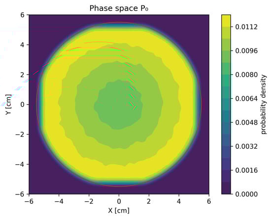
Figure 1.
Contour plot of the marginal distribution of particle X and Y coordinates for phase space . The red circle of radius cm denotes the area outside of which particles in phase spaces were rejected for GAN training.
Tests of the InfoVAE model were conducted for only one phase space with an average energy of MV, focal spot size 1 mm, and beam divergence 0. The training space consisted of 6 million photons and the test space of 4 million photons.
2.6. Evaluation
In GAN training, generic measures of the discrepancy between distributions of random variables must be applied. However, the final evaluation should be performed using clinically relevant figures of merit. To this end, lateral and depth dose profiles in a water phantom of size 40 cm × 40 cm × 40 cm were compared for spatial dose distributions calculated with MC-based and GAN-based phase spaces. The dose distributions in the water phantoms were calculated for three open radiation fields [7]: 30 cm × 30 cm, 10 cm × 10 cm, and 3 cm × 3 cm.
Four different radiotherapy plans were also considered. Two of these were IMRT prostate plans: a clinical plan described elsewhere [21], denoted P1, and a plan based on the I2 test taken from the AAPM TG-119 report [22], and denoted P2. The second plan (P2) was also recalculated with respect to the I’mRT phantom® (IBA Dosimetry, Walloon Brabant, Belgium). The other two radiotherapy plans were VMAT head and neck plans—a clinical one based on patient HN-HGJ-092 from the Head-Neck-PET-CT collection [23,24], denoted HN1, and another, denoted as HN2, based on the I3 test from the AAPM TG-119 report. This second plan was recalculated for the Alderson Rando phantom. For each predefined structure in each plan, dose–volume histograms (DVH) [25] and gamma passing rates (GPR) [26] were calculated and evaluated.
3. Results
Within the model validation process, we evaluated the differences in the probability density distributions of the PRIMO-generated and GAN-generated phase spaces, and next applied the standard quality figures of merit to selected radiotherapy plans.
3.1. Evaluation of Probability Distributions
In Figure 2, we show histograms of the one-dimensional marginal distributions of the test phase spaces. The histograms were calculated using Gaussian kernel density estimation. Medians and quartiles of the probability densities were also calculated. Differences between density estimates for PRIMO-generated and GAN-generated distributions were calculated for each tested space. Next, the medians of the absolute differences between these estimates were calculated, as well as the first and third quartiles, independently at each parameter value.
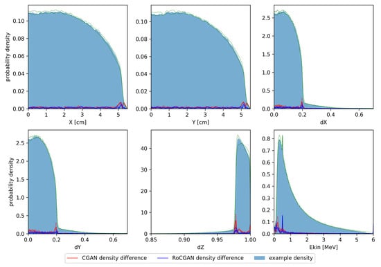
Figure 2.
Histograms of test phase spaces. Solid color denotes median of kernel density estimates for training and test phase spaces, respectively. Green dashed lines denote first and third quartiles of probability densities. Solid lines denote median absolute differences between PRIMO-generated and GAN-generated probability estimates. Dashed lines correspond to first and third quartiles of absolute differences.
In Figure 3, we present the same types of distributions obtained in the same manner as those presented in Figure 2, but using the trained InfoVAE model. Although this model is able to capture the overall shapes of the respective marginal distributions, the differences are clearly larger than those observed in the case of the GAN model.
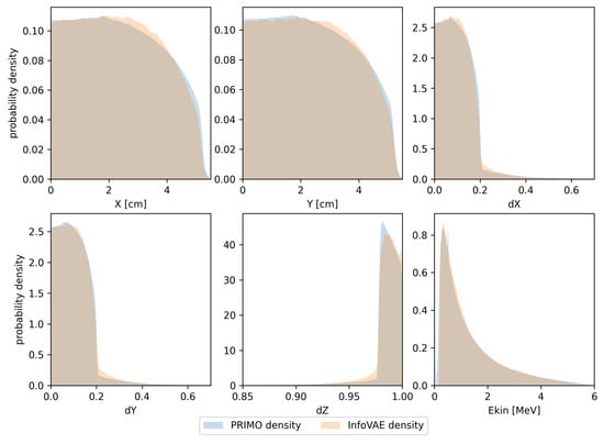
Figure 3.
Probability density estimates for the training space used in the InfoVAE model. Densities calculated from PRIMO-generated phase space are depicted in blue, while densities for the InfoVAE-generated phase space are shown in orange.
3.2. Evaluation of Dose Distributions
Results of water phantom validation are shown in Figure 4. Root mean squared differences (denoted RMS) between profiles generated from the PRIMO phase spaces and GAN phase spaces were calculated for all test settings. Some profiles with the largest and smallest differences are shown in Figure 4. Depth profiles were computed along the beam axis, where the phase space with the highest error was for the CGAN model and for the RoCGAN model. The lateral profiles were computed along the Y axis at cm depth, which was greater than the depth at which the maximum dose occurred and represented about 80% of the maximum dose. In this case, the phase spaces with the highest errors were for the CGAN model and for the RoCGAN model, respectively.
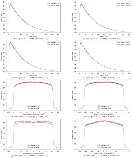
Figure 4.
Dose profiles calculated from the PRIMO-generated phase space and GAN-generated phase space, with bands representing two standard deviations of dose uncertainty, as reported by PRIMO. (a–d) Depth profiles at beam axis. (e–h) Lateral profiles along the Y axis at depth cm. In panels (a,b,e,f) are shown profiles for which the RMS value was the lowest among all test phase spaces. The remaining four profiles are those for which the corresponding RMS value was the highest. All profiles have been normalized to 1.0 relative dose at cm beam depth in water.
Next, gamma passing rates (GPR) for 2%/2 mm tolerance [26] and relative dose differences to 5% and 95% of the region volume (denoted, respectively, and ) [25] in selected regions of interest were calculated for each phase space and plan. These regions included the planned target volume (PTV), gross target volume (GTV), clinical target volume (CTV), brain, brain stem, spinal cord, prostate, mandible, and submandibular glands. Relative dose differences to were calculated as , where is the smallest reference dose to be received in the most irradiated volume; similarly, refers to the same quantity in the compared dose distribution. Results are presented in Table 2 for both models. In an ideal situation, the GPR is equal to 100% and relative dose differences are equal to 0%.
Table 2.
Evaluation of the CGAN and RoCGAN models as applied to radiotherapy plans. Average 2%/2 mm gamma passing rates and relative absolute differences in and overall PTV and OAR ROIs have been set. The last row contains the p-value of the Wilcoxon signed-rank test for equality of mean values of respective columns for CGAN and RoCGAN models. All quantities except p-values are given in percent.
The speed of phase space generation was compared by the requirement to generate 350 million photons to the given phase space. PRIMO required about 24 h on 48 CPU cores to complete the task with splitting roulette variance reduction activated. With this option disabled, the time increased to 60 h on 48 CPU cores. The RoCGAN model can generate a phase space of the same size in about 1 h on a single CPU core; thus, the GAN generates photons over 1000-times faster than MC with variance reduction and over 2800-times faster than MC without variance reduction.
4. Discussion
In this study, conditional generative adversarial networks were proposed to learn the joint multidimensional probability density distribution of the properties of photons (location in space, energy, and momentum) included in the phase spaces of medical linear accelerator simulators. Because the networks are conditioned with respect to the parameters of the primary electron beam (unique to individual medical linear accelerators), the trained models are generic and can be used to generate phase spaces for arbitrary parameters of the primary electron beam within the limits over which the training data were collected.
Histograms shown in Figure 2 demonstrate that differences between the PRIMO-generated and GAN-generated phase spaces are much smaller than the densities themselves, with a few exceptions related to areas with large gradients of probability density. Notably, the high variability of density between phase spaces exhibited by the Z component of momentum is well reflected by the RoCGAN model.
Doses delivered to a water phantom calculated based on the RoCGAN-generated phase spaces closely match the doses from PRIMO-generated phase spaces. As seen in Figure 4, differences in delivered dose, even in the worst case, are not much larger than their statistical uncertainty in the case of lateral profiles and within statistical uncertainty for depth profiles. As indicated by the p-values of the Wilcoxon signed-rank test in Table 3, the CGAN and RoCGAN models have similar levels of error for depth profiles. For the lateral dose profiles, the RoCGAN model delivers a significantly lower level of error with respect to MC-based profiles.
Table 3.
RMS distances between dose distributions in a water phantom for different open field sizes. The first three groups of columns correspond to lateral profiles for different field sizes and the last two columns correspond to the depth profile of the 30 cm × 30 cm field. Values are given as percentage of the maximum dose in the profile calculated from PRIMO-generated phase space. The ’mean’ and ’std’ rows contain, respectively, the mean and standard deviation of values in their respective columns. The last row contains the p-value of the Wilcoxon signed-rank test for equality of mean values of RMS for CGAN and RoCGAN models.
Importantly, any loss of accuracy due to the application of machine learning models does not significantly affect the predicted dose distributions in test plans P1, P2, HN1, and HN2, as demonstrated by the high gamma passing rates and low dose differences in Table 2. For the P1 plan, the CGAN and RoCGAN models work equally well, as judged from the p-values in Table 2, but for the remaining three plans, the RoCGAN model delivers a significantly lower level of error.
The results of simulating dose delivery to water phantoms, to test phantoms, and to patients indicate that the MC-based and GAN-based phase spaces can, in most cases, be used interchangeably. Because the generation of particles with GANs is 1000-times faster than that with MC, GANs can be used on the fly to increase the amount of particles in the phase space, thus improving the precision of dose calculation in phantoms or in patients.
The universality of the conditional GANs was achieved at the cost of handling a large volume of training data—almost 570 MC phase spaces, each containing some particles, were generated. This resulted in some TB of data collected. Such a massive simulation campaign could not be completed without the grid infrastructure of our University.
As mentioned in the Introduction, we decided not to use variance reduction techniques when preparing the training data for conditional GANs. This decision was made after a comprehensive series of experiments aimed at reproducing the results of [8] based on phase spaces generated with variance reduction techniques. Because these experiments were not successful, we decided to collect MC training data with variance reduction switched off. After the successful reproduction of the results of Sarrut, Krah, and Letang [8] with such data, we were able to extend their work to the application of conditional GANs. Arguably, one could try to retrieve discrete weights that are assigned to phase space particles when using variance reduction, from continuous outputs of GANs—this is how the classification task is solved with deep models. However, the outputs of classification networks can be interpreted as probabilities, which guide the assignment of discrete classes to classified objects, based on continuous outputs. This is not the case for phase spaces, which is another argument not to use variance reduction when preparing training data for our GAN models.
The same arguments concerning the continuity of the learnt probability distributions led us to remove annihilation photons from the training data. The absence of these photons in GAN-generated phase spaces is clearly visible in Figure 2. Of course, one may train some regression model to predict how the fraction of annihilation photons in phase spaces depends on the parameters of the electron beam. One may also fit the probability density functions of the parameters of these photons (except their energy, which is fixed). The results of this study demonstrate, however, that the absence of annihilation photons in GAN-generated phase spaces does not affect the dose distributions in either phantoms or patients.
Note that in the description of the architectures used in this study, some values of hyperparameters were mentioned, such as the number of neurons in dense layers, equal to 400, or the dimensionality of the noise vector at the input of the generator, equal to 8. These parameters were reported in the study of Sarrut, Krah, and Letang [8] as being optimal for the task of photon generation and, for this reason, were also used in our study. Because the models described in this study are extensions of their model, the optimal hyperparameters of our model may differ from the optimal hyperparameters reported for their GAN model. The results found for the hyperparameters that they suggested [8] are, however, sufficient to justify our decision not to search for any better hyperparameters.
The model that we propose is more general than other approaches to fast and efficient phase space generation. For example, Tian et al. [27], in their GPU-based approach, assume rotational symmetry of their phase space—which need not apply in the case that we consider. GAN-based modeling could also be considered as an alternative in modeling particle therapy, as shown, e.g., by Wang et al. [28]. A general drawback of GAN-based modeling is, however, the limited possibility of robust error estimation—unlike in analytical and Monte Carlo calculations. The legal and ethical issues that increasingly accompany advances in artificial intelligence techniques in medical diagnostics and therapy—including radiotherapy–should also be acknowledged [29].
In addition to GANs, we evaluated several other types of models in our initial investigations. We finally rejected them either as not being accurate enough (such as models based on the variational autoencoder approach) or because we found the process of particle generation too slow for the intended purpose of the model (for example, continuous normalizing flow models). We also paid considerable attention to models of the variational autoencoder family. Although such models were able to generate realistic phase spaces (in particular, the InfoVAE model discussed in this work), their results, already for one training space (nonconditional), were of lower quality than those of the CGAN or RoCGAN models. In addition, the use of the MMD member in the loss function entailed a much higher computational cost of training the model than that for models of the GAN family. This led us to reject this family of generative models.
5. Conclusions
A fast machine-learning-based method for the generation of phase spaces in a linac at the level below the flattening filter was presented in this study. The trained model can produce particle data for different initial values of electron energy, focal spot size, and beam divergence of the linac, much more quickly than the present Monte Carlo simulations. Results of the evaluation of phase spaces generated in such a manner indicate that such phase spaces are sufficiently accurate for the purposes of simulating further stages of dose delivery in a radiotherapy system.
Author Contributions
Conceptualization, Z.T. and D.S.; Methodology, Z.T.; Software, D.S. and Z.T.; Validation, K.R.; Formal Analysis, M.B.; Investigation, Z.T. and M.B.; Resources, K.R.; Data Curation, K.R.; Writing—Original Draft Preparation, M.B. and Z.T.; Writing—Review and Editing, M.B., M.P.R.W., P.Z., T.S., K.K., J.M. and B.R.; Visualization, M.B.; Supervision, M.P.R.W. and K.R.; Project Administration, K.R.; Funding Acquisition, T.S. All authors have read and agreed to the published version of the manuscript.
Funding
The project was supported by the TEAM-NET program of the Foundation for Polish Science, co-financed by the European Union under the European Regional Development Fund (POIR.04.04.00-00-15E5/18). This research was supported by PLGrid Infrastructure.
Institutional Review Board Statement
Not applicable.
Informed Consent Statement
Not applicable.
Data Availability Statement
The data presented in this study are available on request from the corresponding author.
Acknowledgments
The authors wish to thank Łukasz Flis of the ACC Cyfronet AGH for his invaluable help in handling computations on the Prometheus grid.
Conflicts of Interest
The authors declare no conflict of interest. The funders had no role in the design of the study; in the collection, analyses, or interpretation of data; in the writing of the manuscript; or in the decision to publish the results.
References
- Foster, I.; Spezi, E.; Wheeler, P. Evaluating the Use of Machine Learning to Predict Expert-Driven Pareto-Navigated Calibrations for Personalised Automated Radiotherapy Planning. Appl. Sci. 2023, 13, 4548. [Google Scholar] [CrossRef]
- Storchi, P.; Woudstra, E. Calculation of the absorbed dose distribution due to irregularly shaped photon beams using pencil beam kernels derived form basic beam data. Phys. Med. Biol. 1996, 41, 637–656. [Google Scholar] [CrossRef] [PubMed]
- Ulmer, W.; Pyyry, J.; Kaissl, W. A 3D photon superposition/convolution algorithm and its foundation on results of Monte Carlo calculations. Phys. Med. Biol. 2005, 50, 1767–1790. [Google Scholar] [CrossRef]
- Failla, G.; Wareing, T.A.; Archambault, Y.; Thompson, S. XB advanced dose calculation for the Eclipse treatment planning system. Varian Med. Syst. 2010, 20, 18. [Google Scholar]
- Chetty, I.J.; Curran, B.; Cygler, J.E.; DeMarco, J.J.; Ezzell, G.; Faddegon, B.A.; Kawrakow, I.; Keall, P.J.; Liu, H.; Ma, C.M.C.; et al. Report of the AAPM Task Group No. 105: Issues associated with clinical implementation of Monte Carlo-based photon and electron external beam treatment planning. Med. Phys. 2007, 34, 4818–4853. [Google Scholar] [CrossRef]
- Seco, J.; Verhaegen, F. Monte Carlo Techniques in Radiation Therapy; CRC Press: Boca Raton, FL, USA, 2013. [Google Scholar]
- Tabor, Z.; Kabat, D.; Waligórski, M.P.R. DeepBeam: A machine learning framework for tuning the primary electron beam of the PRIMO Monte Carlo software. Radiat. Oncol. 2021, 16, 124. [Google Scholar] [CrossRef] [PubMed]
- Sarrut, D.; Krah, N.; Létang, J.M. Generative adversarial networks (GAN) for compact beam source modelling in Monte Carlo simulations. Phys. Med. Biol. 2019, 64, 215004. [Google Scholar] [CrossRef] [PubMed]
- Stevens, E.; Antiga, L.; Viehmann, T. Deep Learning with PyTorch: Build, Train, and Tune Neural Networks Using Python Tools, 1st ed.; Manning: Shelter Island, NY, USA, 2020. [Google Scholar]
- Burkhardt, J. Bayesian Parameter Inference of Explosive Yields Using Markov Chain Monte Carlo Techniques. Int. J. Math. Sci. Comput. 2020, 6, 1–17. [Google Scholar] [CrossRef]
- Husaini, N.A.; Ghazali, R.; Arbaiy, N.; Lasisi, A. MCS-MCMC for Optimising Architectures and Weights of Higher Order Neural Networks. Int. J. Intell. Syst. Appl. 2020, 12, 52–72. [Google Scholar] [CrossRef]
- Izonin, I.; Tkachenko, R.; Fedushko, S.; Koziy, D.; Zub, K.; Vovk, O. RBF-Based Input Doubling Method for Small Medical Data Processing. In Proceedings of the Advances in Artificial Systems for Logistics Engineering, Kiev, Ukraine, 22–24 January 2021; Hu, Z., Zhang, Q., Petoukhov, S., He, M., Eds.; Lecture Notes on Data Engineering and CommunicationsTechnologies. Springer: Cham, Switzerland, 2021; pp. 23–31. [Google Scholar] [CrossRef]
- Rodriguez, M.; Sempau, J.; Brualla, L. PRIMO: A graphical environment for the Monte Carlo simulation of Varian and Elekta linacs. Strahlenther. Onkol. 2013, 189, 881–886. [Google Scholar] [CrossRef]
- Rodriguez, M.; Sempau, J.; Brualla, L. A combined approach of variance-reduction techniques for the efficient Monte Carlo simulation of linacs. Phys. Med. Biol. 2012, 57, 3013–3024. [Google Scholar] [CrossRef] [PubMed]
- Arjovsky, M.; Chintala, S.; Bottou, L. Wasserstein Generative Adversarial Networks. In Proceedings of the 34th International Conference on Machine Learning, Sydney, Australia, 6–11 August 2017; pp. 214–223, ISSN 2640–3498. [Google Scholar]
- Atienza, R. Advanced Deep Learning with TensorFlow 2 and Keras: Apply DL, GANs, VAEs, Deep RL, Unsupervised Learning, Object Detection and Segmentation, and More, 2nd ed.; Packt Publishing: Birmingham, UK, 2020. [Google Scholar]
- Chrysos, G.G.; Kossaifi, J.; Zafeiriou, S. RoCGAN: Robust Conditional GAN. Int. J. Comput. Vis. 2020, 128, 2665–2683. [Google Scholar] [CrossRef]
- Kingma, D.P.; Welling, M. Auto-encoding variational bayes. arXiv 2013, arXiv:1312.6114. [Google Scholar]
- Zhao, S.; Song, J.; Ermon, S. InfoVAE: Information Maximizing Variational Autoencoders. arXiv 2017, arXiv:1706.02262. [Google Scholar]
- Gretton, A.; Borgwardt, K.M.; Rasch, M.J.; Schölkopf, B.; Smola, A. A kernel two-sample test. J. Mach. Learn. Res. 2012, 13, 723–773. [Google Scholar]
- Baran, M.; Tabor, Z.; Tulik, M.; Kabat, D.; Rzecki, K.; Sośnicki, T.; Waligórski, M. Are gamma passing rate and dose-volume histogram QA metrics correlated? Med. Phys. 2021, 48, 4743–4753. [Google Scholar] [CrossRef]
- Ezzell, G.A.; Burmeister, J.W.; Dogan, N.; LoSasso, T.J.; Mechalakos, J.G.; Mihailidis, D.; Molineu, A.; Palta, J.R.; Ramsey, C.R.; Salter, B.J.; et al. IMRT commissioning: Multiple institution planning and dosimetry comparisons, a report from AAPM Task Group 119. Med. Phys. 2009, 36, 5359–5373. [Google Scholar] [CrossRef]
- Vallières, M.; Kay-Rivest, E.; Perrin, L.J.; Liem, X.; Furstoss, C.; Aerts, H.J.W.L.; Khaouam, N.; Nguyen-Tan, P.F.; Wang, C.S.; Sultanem, K.; et al. Radiomics strategies for risk assessment of tumour failure in head-and-neck cancer. Sci. Rep. 2017, 7, 10117. [Google Scholar] [CrossRef]
- Clark, K.; Vendt, B.; Smith, K.; Freymann, J.; Kirby, J.; Koppel, P.; Moore, S.; Phillips, S.; Maffitt, D.; Pringle, M.; et al. The Cancer Imaging Archive (TCIA): Maintaining and Operating a Public Information Repository. J. Digit. Imaging 2013, 26, 1045–1057. [Google Scholar] [CrossRef]
- Drzymala, R.E.; Mohan, R.; Brewster, L.; Chu, J.; Goitein, M.; Harms, W.; Urie, M. Dose-volume histograms. Int. J. Radiat. Oncol. Biol. Phys. 1991, 21, 71–78. [Google Scholar] [CrossRef]
- Low, D.A.; Harms, W.B.; Mutic, S.; Purdy, J.A. A technique for the quantitative evaluation of dose distributions. Med. Phys. 1998, 25, 656–661. [Google Scholar] [CrossRef] [PubMed]
- Tian, Z.; Li, Y.; Folkerts, M.; Shi, F.; Jiang, S.B.; Jia, X. An analytic linear accelerator source model for GPU-based Monte Carlo dose calculations. Phys. Med. Biol. 2015, 60, 7941. [Google Scholar] [CrossRef] [PubMed]
- Wang, Q.; Zhu, C.; Bai, X.; Deng, Y.; Schlegel, N.; Adair, A.; Chen, Z.; Li, Y.; Moyers, M.; Yepes, P. Automatic phase space generation for Monte Carlo calculations of intensity modulated particle therapy. Biomed. Phys. Eng. Express 2020, 6, 025001. [Google Scholar] [CrossRef]
- Santoro, M.; Strolin, S.; Paolani, G.; Della Gala, G.; Bartoloni, A.; Giacometti, C.; Ammendolia, I.; Morganti, A.G.; Strigari, L. Recent Applications of Artificial Intelligence in Radiotherapy: Where We Are and Beyond. Appl. Sci. 2022, 12, 3223. [Google Scholar] [CrossRef]


Disclaimer/Publisher’s Note: The statements, opinions and data contained in all publications are solely those of the individual author(s) and contributor(s) and not of MDPI and/or the editor(s). MDPI and/or the editor(s) disclaim responsibility for any injury to people or property resulting from any ideas, methods, instructions or products referred to in the content. |
© 2023 by the authors. Licensee MDPI, Basel, Switzerland. This article is an open access article distributed under the terms and conditions of the Creative Commons Attribution (CC BY) license (https://creativecommons.org/licenses/by/4.0/).