Leader–Follower Formation Tracking Control of Underactuated Surface Vehicles Based on Event-Trigged Control

Abstract

This paper investigates the leader–follower formation tracking control of underactuated surface vessels (USVs) with input saturation. Each vessel is subject to the uncertainties induced by model uncertainties and environmental disturbances. First, an event-triggered extended-state observer (ETESO) is used to recover the velocity, yaw rate and uncertainties. Then, an estimator is used to estimate the velocity of the leader. An event-triggered controller (ETC) is constructed based on the estimator, the observer and extra variables. Specifically, extra variables are used to solve the problems of underactuation and input saturation. Stability analysis of the control system is conducted to prove that all signals are bounded. Simulations demonstrate that the ETESO can accurately estimate the uncertainties, velocity and yaw rate, and the ETC can largely reduce the action times of actuator.

1. Introduction

In recent years, formation tracking control of underactuated surface vessels (USVs) has attracted considerable interest, as USVs can be widely used in ocean engineering fields [1,2,3]. Compared with single vessels, formations offer many advantages. In the course of ocean exploration, the efficiency of a single vessel is low, whereas formations can perform the complex tasks such as pursuit tasks that usually cannot be accomplished by a single vessel. There are various formation control schemes, including the leader–follower approach [4,5], virtual structure [6], the graph-based mechanism [7], the data-driven model [8], UAV–USV heterogeneous multiagent systems [9] and adaptive fuzzy formation control [10]. In particular, the leader–follower strategy is preferred in ocean engineering applications. The follower maintains a desired distance and angle relative to the leader, and a reference trajectory can be defined by the leader. Therefore, the group behavior is directed by the leader, and the formation stability can be induced by the control law of a single vessel.

There are two main challenges that are still worth mentioning. The first challenge is actuator saturation, which can severely degrade the closed-loop system performance [11]. In practice, each actuator of a vessel can only provide a limited force or torque. To reduce the risk of actuator saturation and enhance system performance, some methods have been proposed in recent years. To avoid poor tracking performance in formation control, generalized saturation functions combined with formation tracking errors were employed to handle the input saturation problem [12]. To solve the problems of input saturation and underactuation simultaneously, additional variables were induced to velocity errors in the body-fixed frame [13,14]. Non-linear saturation of an actuator was approximated by a Gaussian error function [15] such that an anti-saturation controller could be designed. An auxiliary dynamic system was constructed to solve the input saturation problem [16], with the auxiliary dynamic system designed as a second-order system, providing a conservative input signal. A first-order auxiliary system was designed in [17] and employed to deal with input saturation of the rudder. The authors of [18] used an auxiliary system to solve the problem of input saturation, which was combined with a collision-avoidance control strategy to provide tracking control for dynamic vessel positioning. However, the limited acting frequency actuators was not considered in the articles mentioned above.

High-frequency action may lead not only to mechanical abrasion but also to a short service life [19]. Input saturation and actuator rate limits were considered in [20], and a non-linear controller was designed based on dynamic surface control and backstepping technology. Additional controllers were proposed to deal with actuator magnitude and rate saturation in [21]. The authors of [22] considered actuator saturation with limited magnitude and rate and designed a sliding model controller. In [20,21,22], Zeno behavior was avoided because the acting frequency of actuator was bounded. A controller combined with an event-triggered condition was proposed in [23], and the triggered condition was designed based on the flow time and error function; however, this configuration still resulted in long action times of the actuator. An event-triggered distributed controller was employed in [24], and the triggered condition was designed based on changes in amplitude of input signals. The authors of [25] proposed an event-triggered control law, and an event-triggered mechanism was used to reduce the execution frequency of actuators. The event-triggered mechanism was designed in the controller-to-actuator channel, and the execution rate of the actuator was reduced.

The second significant challenge is the uncertainties. Because of the working condition of the surface vessel, uncertainties include model uncertainties and environmental disturbances. In [26], the proposed controller was robust to the parameter uncertainties of the nonlinear terms and exogenous disturbances. Unknown plant parameters and environmental disturbances were solved using parameter estimation and upper-bound estimation in [27]. In [28], a robust adaptive control algorithm was proposed to solve uncertain parameters. Adaptive estimators were designed to estimate unknown time-varying functions of vessel model in [29]. Considering the leader–follower formation tracking problem, a neural network was used to approximate the uncertainties, and the uncertainties were compensated by online learning [30]. A cooperative controller was proposed using position-heading measurements in [31], and an extended-state observer (ESO) was constructed to provide the estimations of velocity, yaw rate and uncertainties. However, the existing observers presented in [14,16,19,25,31,32] relied on continuous sampling. In each execution cycle, signals are transmitted, which means that many network resources and calculation resources are consumed. To avoid unnecessary calculation and communication, an event-triggered extended-state observer (ETESO) was proposed in [33]. In [34], an ETESO was proposed for a class of non-linear networked control systems, and the state estimation problem was solved. As for USVs, when the working mode is tracking control, in most cases, the yaw angle is unchanged. In the common continuous observer, the signals have to be transmitted during each execution cycle, consuming many network resources and calculation resources. Therefore, it is rewarding to design a leader–follower tracking controller with a light transmission load and short action times of actuators.

Based on the above research background, in this paper, we investigate leader–follower formation tracking control of USVs subject to input saturation, model uncertainties and environmental disturbances. Inspired by the work reported in [23,31], an improved output feedback controller was proposed. First, an ETESO was used to recover the velocity data and model uncertainties and disturbances. In each execution cycle, an event-triggered strategy is monitored to determine whether or not to transmit the position and head information to the observer. Sensor-to-observer communication costs are drastically reduced. Secondly, an estimator is employed to estimate the velocity of the leader and reduce the amount of data exchanged in formation. Thirdly, auxiliary variables provide a solution for the problems of input saturation and underactuation. Then, an event-triggered controller (ETC) was designed based on the ETESO, the estimator and auxiliary variables. Finally, the stability of the closed-loop system was proven. Simulations were also conducted to demonstrate the proposed control strategy.

Two salient features of the proposed control are summarized as follows. First, an estimator is employed to estimate the velocity of the leader, the embedded processor of each follower performs reading computations only using the position and yaw of the leader and the transmission loads between formations are saved. Second, an event-triggered mechanism is designed in the controller-to-actuator channel, and action times of actuator are reduced.

Compared with the existing related results, the novelty of this paper is summarized as follows. First, in contrast to existing formation control approaches [25,31], the velocity of the leader is estimated by an estimator, which reduces the amount of data exchanged between USVs. Second, compared with the observer proposed in [31], the ETESO can reduce sensor-to-observer communication costs. Third, compared with the strategy proposed in [23], the proposed control law can largely reduce the action times of the actuator.

The remainder of this paper is organized as follows. A list of notations defining variables used in this paper is presented in

Table 1. Notations and variables used in this paper.

${\mathbb{R}}^n$	n-dimensional Euclidean space
$|·|$	Absolute value of a variable
${\lambda }_{min}(·)$	Minimum eigenvalue of a matrix
$min\{·\}$	Minimum value of a set
inf $\{·\}$	Supremum of a set
${(·)}^T$	Transpose of a matrix
$\parallel ·\parallel$	Euclidean norm of a vector
$\mathrm{diag}\{·\}$	Diagonal matrix
$I_n$	$n\times n$ dimensional identity matrix
$0_n$	$n\times n$ dimensional zero matrix.
$(x_i,y_i)$, ${\psi }_i$, $(x_j,y_j)$, ${\psi }_j$	Position and yaw of the ith USV and the leader (j)
$u_i$, $v_i$, $r_i$, $u_j$, $v_j$, $r_j$	Surge velocity, sway velocity and yaw rate of the ith USV and the leader (j)
$m_{i,11}$, $m_{i,22}$, $m_{i,33}$	Inertia mass of the ith USV
${\sigma }_{i,h}$	Hydrodynamic damping parameters and disturbances
${\tau }_i=[{\tau }_{i,u},0,{\tau }_{i,r}]$	Input signals of the ith USV
${\eta }_i$, ${\nu }_i$	${\eta }_i={[x_i,y_i,{\psi }_i]}^T$, ${\nu }_i={[u_i,v_i,r_i]}^T$
${\eta }_j$, ${\nu }_j$	${\eta }_j={[x_j,y_j,{\psi }_j]}^T$, ${\nu }_j={[u_j,v_j,r_j]}^T$
$M_i$	$M_i=\mathrm{diag}\{m_{i,11},m_{i,22},m_{i,33}\}$
$R_i$	Rotation matrices of the ith USV
${\tau }_{ic}={[{\tau }_{i,uc},0,{\tau }_{i,rc}]}^T$	${\tau }_{ic}$ calculated by the proposed controller
${\varpi }_i={[{\varpi }_{i,u},0,{\varpi }_{i,r}]}^T$	The mismatch function between input without saturation and input with saturation
${\rho }_{ij}$, ${\lambda }_{ij}$	Relative distance and angle between the ith USV and the leader (j)
${\rho }_{ij,d}$, ${\lambda }_{ij,d}$	Desired distance and angle
$\widehat{x}$	Estimate of variable x
$t_k$	Previous event-triggering time instant
${\xi }_i$	Transmitted signal between ${\eta }_i\left(t\right)$ and ${\eta }_i\left(t_k\right)$
$d\left(t\right)$	Event-triggered mechanism
$\tilde{x}=\widehat{x}-x$	Estimation error of variable x
$P_{ij}={[{\rho }_{ij,e},{\lambda }_{ij,e}]}^T$	Formation tracking error vector
${\widehat{\Theta }}_i$	Estimator used to estimate velocity of the leader
$l_{i,h}$	Time constants of the first-order filters
${\psi }_{i,e}$	Yaw tracking error
${\beta }_{i,h}$	Virtual controls
${\alpha }_{i,h}$	Auxiliary variables
${\omega }_{i,h}$	Errors caused by the first-order filter
${\omega }_{\tau u}$, ${\omega }_{\tau r}$	Control laws at the kinetic level

. Section 2 describes the preliminaries and problem formulation. Section 3 describes observer design, and Section 4 presents the controller design and a stability analysis. Simulation results are presented in Section 5. Section 6 concludes this paper.

2. Problem Formulation

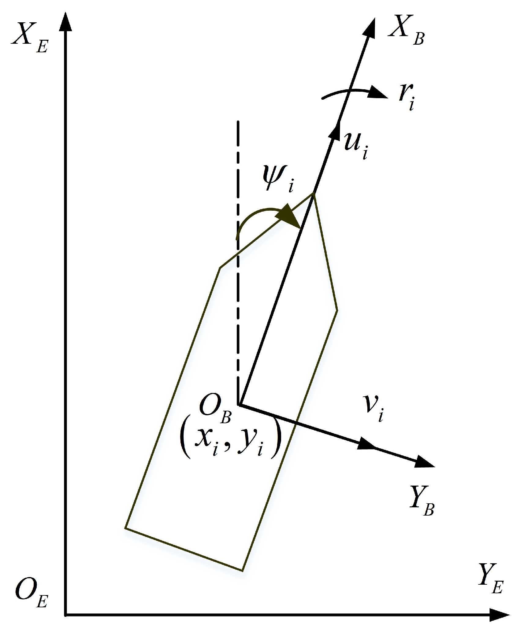
As shown in Figure 1, a group of USVs consists of N USVs, and the model of the ith USV is given as [35]

$$\begin{array}{cc}\hfill {\dot{x}}_i& =u_i\cos \left({\psi }_i\right)-v_i\sin \left({\psi }_i\right),\hfill \end{array}$$

(1)

$$\begin{array}{cc}\hfill {\dot{y}}_i& =u_i\sin \left({\psi }_i\right)+v_i\cos \left({\psi }_i\right),\hfill \end{array}$$

(2)

$$\begin{array}{cc}\hfill {\dot{\psi }}_i& =r_i,\hfill \end{array}$$

(3)

and

$${\dot{u}}_i={\sigma }_{i,1}+\frac{1}{m_{i,11}}{\tau }_{i,u},$$

(4)

$${\dot{v}}_i={\sigma }_{i,2},$$

(5)

$$\begin{array}{cc}\hfill {\dot{r}}_i& ={\sigma }_{i,3}+\frac{1}{m_{i,33}}{\tau }_{i,r},\hfill \end{array}$$

(6)

where ${(x_i,y_i)}^T\in {\mathbb{R}}^2$ is the position in the Earth-fixed frame ($X_E{O}_E{Y}_E$); ${\psi }_i$ is the yaw angle in $X_E{O}_E{Y}_E$; $u_i$ is the surge velocity in the body-fixed frame ($X_B{O}_B{Y}_B$); $v_i$ is the sway velocity in $X_B{O}_B{Y}_B$; $r_i$ is the yaw rate in $X_B{O}_B{Y}_B$; $m_{i,11}$ and $m_{i,33}$ denote the inertia mass; uncertainties ${\sigma }_{i,1}$, ${\sigma }_{i,2}$ and ${\sigma }_{i,3}$ contain Coriolis parameters, hydrodynamic damping parameters and time-varying disturbances, respectively; and ${\tau }_{i,u}$ and ${\tau }_{i,r}$ are input signals.

To facilitate observer design and analysis, the ith USV model is written as

$${\dot{\eta }}_i=R_i{\nu }_i$$

(7)

$${\dot{\nu }}_i=M_i^{-1}{\tau }_i+{\sigma }_i,$$

(8)

where ${\eta }_i={[x_i,y_i,{\psi }_i]}^T$, ${\nu }_i={[u_i,v_i,r_i]}^T$, ${\tau }_i={[{\tau }_{i,u},0,{\tau }_{i,r}]}^T$, $M_i=\mathrm{diag}\{m_{i,11},m_{i,22},m_{i,33}\}$, $m_{i,22}$ is the inertia mass. ${\sigma }_i={[{\sigma }_{i,1},{\sigma }_{i,2},{\sigma }_{i,3}]}^T$, and

$$R_i=\left[\begin{array}{ccc}\cos \left({\psi }_i\right)& -\sin {\psi }_i)& 0\\ \sin {\psi }_i)& \cos \left({\psi }_i\right)& 0\\ 0& 0& 1\end{array}\right].$$

The mismatch function between input without saturation and input with saturation is described as ${\varpi }_i={[{\varpi }_{i,u},0,{\varpi }_{i,r}]}^T$$={\tau }_{ic}-{\tau }_i$, where ${\tau }_{ic}={[{\tau }_{i,uc},0,{\tau }_{i,rc}]}^T$; ${\tau }_{i,uc}$ and ${\tau }_{i,rc}$ are the surge force and yaw moment calculated by the proposed controller, respectively; and ${\tau }_i={[{\tau }_{i,u},0,{\tau }_{i,r}]}^T$. Then, the saturated control is given by ${\tau }_i={\tau }_{ic}-{\varpi }_i$.

Assumption 1.

The unknown function ${\sigma }_i$ satisfies ${\dot{\sigma }}_i\le {\sigma }_i^{*}$, where ${\sigma }_i^{*}$ is a positive constant.

${\sigma }_i$ is a vector containing velocity, Coriolis parameters, hydrodynamic damping parameters and time-varying disturbances. It is natural to assume that their derivatives are bounded. Control inputs to drive USVs are bounded; therefore, Assumption 1 is reasonable.

Assumption 2.

The velocity of the ith USV is bounded such that $\parallel {\nu }_i\parallel \le {\nu }_i^{*}$, ${\nu }_i^{*}$ is a positive constant.

The control inputs to drive USVs are bounded, and the energy of external disturbances is limited. Therefore, Assumption 2 is reasonable.

Assumption 3.

The desired distance (${\rho }_{ij,d}$) and angle (${\lambda }_{ij,d}$) are bounded.

Assumption 3 means that the desired value is reasonable.

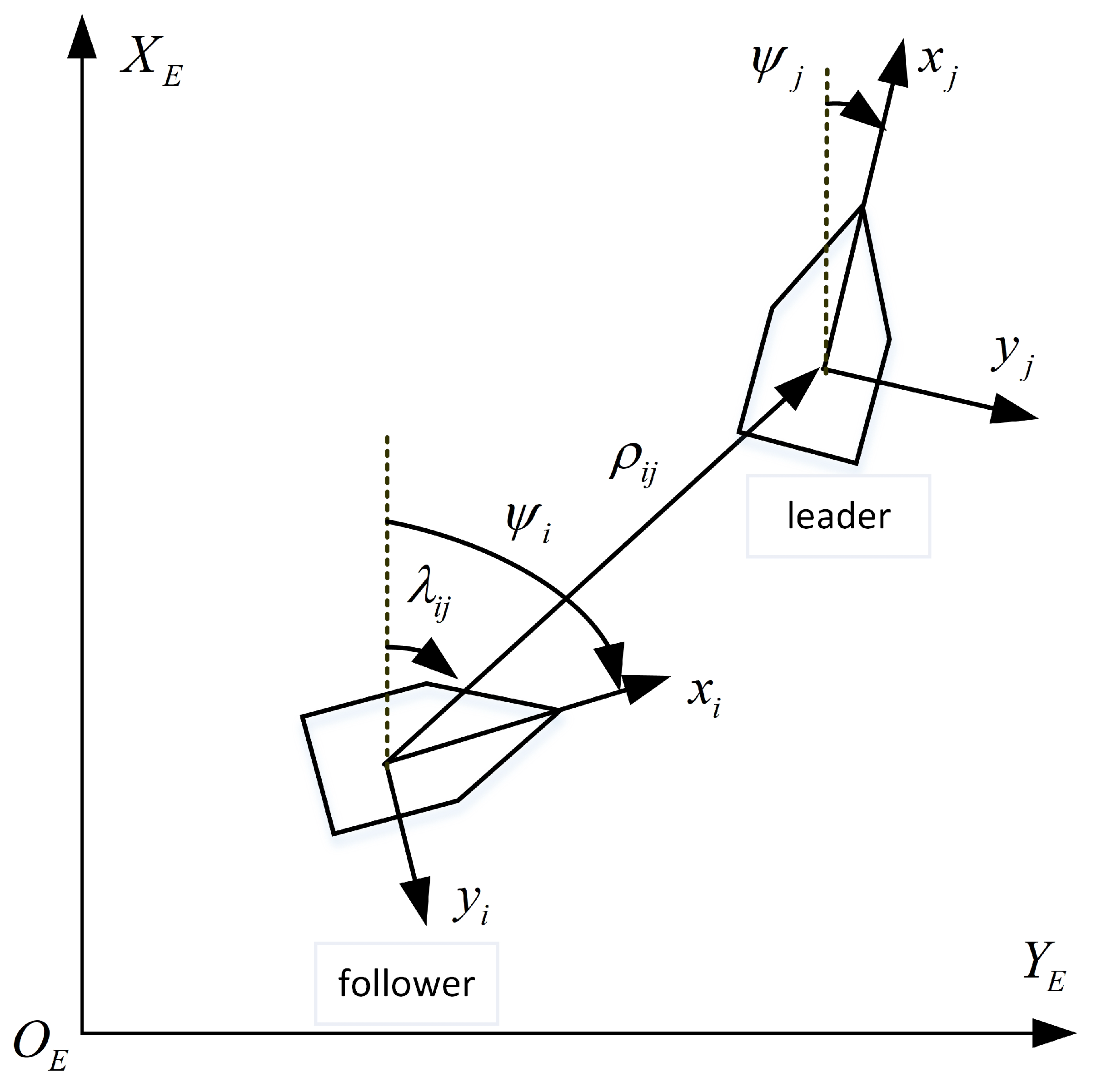
The following definitions are posited.

As shown in Figure 2, the subscript j is the index of the leader (j). ${\eta }_j={[x_j,y_j,{\psi }_j]}^T$ is used to denote the position and yaw of the leader (j). ${\nu }_j={[u_j,v_j,r_j]}^T$ is the velocity and yaw rate of the leader (j).

The relative distance (${\rho }_{ij}$) and angle (${\lambda }_{ij}$) between the ith USV and the leader (j) are expressed as

$$\begin{array}{cc}\hfill {\rho }_{ij}& =\sqrt{{(x_j-x_i)}^2+{(y_j-y_i)}^2},\hfill \end{array}$$

(9)

$$\begin{array}{cc}\hfill {\lambda }_{ij}& =\mathrm{atan}2(y_j-y_i,x_j-x_i).\hfill \end{array}$$

(10)

The differential equations of ${\rho }_{ij}$ and ${\lambda }_{ij}$ are given by:

$$\begin{array}{cc}\hfill {\dot{\rho }}_{ij}=& \frac{(x_j-x_i)({\dot{x}}_j-{\dot{x}}_i)+(y_j-y_i)({\dot{y}}_j-{\dot{y}}_i)}{\sqrt{{(x_j-x_i)}^2+{(y_j-y_i)}^2}}\hfill \end{array}$$

$$\begin{array}{cc}\hfill & =\frac{(x_j-x_i)({\dot{x}}_j-{\dot{x}}_i)+(y_j-y_i)({\dot{y}}_j-{\dot{y}}_i)}{{\rho }_{ij}},\hfill \end{array}$$

(11)

$$\begin{array}{cc}{\dot{\lambda }}_{ij}=\hfill & \frac{1}{1+\frac{{(y_j-y_i)}^2}{{(x_j-x_i)}^2}}\frac{({\dot{y}}_j-{\dot{y}}_i)(x_j-x_i)-({\dot{x}}_j-{\dot{x}}_i)(y_j-y_i)}{{(x_j-x_i)}^2}.\hfill \end{array}$$

(12)

According to $x_j-x_i={\rho }_{ij}cos\left({\lambda }_{ij}\right)$ and $y_j-y_i={\rho }_{ij}sin\left({\lambda }_{ij}\right)$,

$$\begin{array}{cc}\hfill {\dot{\rho }}_{ij}& =[u_{j}cos\left({\psi }_j\right)-v_{j}sin\left({\psi }_j\right)-u_{i}cos\left({\psi }_i\right)+v_{i}sin\left({\psi }_i\right)]cos\left({\lambda }_{ij}\right)\hfill \\ \hfill & +[u_{j}sin\left({\psi }_j\right)+v_{j}cos\left({\psi }_j\right)-u_{i}sin\left({\psi }_i\right)+v_{i}cos\left({\psi }_i\right)]sin\left({\lambda }_{ij}\right)\hfill \\ \hfill & =-u_i\cos ({\psi }_i-{\lambda }_{ij})+u_j\cos ({\psi }_j-{\lambda }_{ij})\hfill \\ \hfill & +v_i\sin ({\psi }_i-{\lambda }_{ij})-v_j\sin ({\psi }_j-{\lambda }_{ij})\hfill \end{array}$$

(13)

$$\begin{array}{cc}\hfill {\dot{\lambda }}_{ij}& =\frac{({\dot{y}}_j-{\dot{y}}_i){\rho }_{ij}cos\left({\lambda }_{ij}\right)-({\dot{x}}_j-{\dot{x}}_i){\rho }_{ij}sin\left({\lambda }_{ij}\right)}{{\rho }_{ij}^2}\hfill \\ \hfill & =\frac{1}{{\rho }_{ij}}\{-u_i\sin ({\psi }_i-{\lambda }_{ij})+u_j\sin ({\psi }_j-{\lambda }_{ij})\hfill \\ \hfill & -v_i\cos ({\psi }_i-{\lambda }_{ij})+v_j\cos ({\psi }_j-{\lambda }_{ij})\}.\hfill \end{array}$$

(14)

The control objective is to design an event-triggered control law for USVs to track the leader with a desired distance (${\rho }_{ij,d)}$ and angle (${\lambda }_{ij,d}$).

Remark 1.

In the controller design process, the ith USV tracks the the jth USV using the $x_j$, $y_j$ and ${\psi }_j$ information. This means that communication costs are not saved between multiple USVs.

3. Event-Triggered Extended-State Observer

An ETESO was developed to estimate uncertainties including model uncertainties and time-varying disturbances, and an event-triggered condition was employed to avoid unnecessary communications. Inspired by [33], an ETESO was designed as follows:

$$\begin{array}{cc}\hfill {\dot{\widehat{\eta }}}_i\left(t\right)=& -\frac{3}{{ϵ}_i}({\widehat{\eta }}_i-{\xi }_i)+R_i{\widehat{\nu }}_i,\hfill \end{array}$$

(15)

$$\begin{array}{cc}\hfill {\dot{\widehat{\nu }}}_i\left(t\right)=& -\frac{3}{{ϵ}_i^2}{R}_i^T({\widehat{\eta }}_i-{\xi }_i)+{\widehat{\sigma }}_i+M_i^{-1}{\tau }_i,\hfill \end{array}$$

(16)

$$\begin{array}{cc}\hfill {\dot{\widehat{\sigma }}}_i\left(t\right)=& -\frac{1}{{ϵ}_i^3}{R}_i^T({\widehat{\eta }}_i-{\xi }_i),\hfill \end{array}$$

(17)

where ${\widehat{\eta }}_i={[{\widehat{x}}_i,{\widehat{y}}_i,{\widehat{\psi }}_i]}^T$; ${\widehat{\nu }}_i={[{\widehat{u}}_i,{\widehat{v}}_i,{\widehat{r}}_i]}^T$; and ${\widehat{\sigma }}_i={[{\widehat{\sigma }}_{i,1},{\widehat{\sigma }}_{i,2},{\widehat{\sigma }}_{i,3}]}^T$; ${\widehat{x}}_i,{\widehat{y}}_i,{\widehat{\psi }}_i,{\widehat{u}}_i,{\widehat{v}}_i,{\widehat{r}}_i,{\widehat{\sigma }}_{i,1},{\widehat{\sigma }}_{i,2}$ and ${\widehat{\sigma }}_{i,3}$ are the estimates of $x_i,y_i,{\psi }_i,u_i,v_i,r_i,{\sigma }_{i,1},{\sigma }_{i,2}$ and ${\sigma }_{i,3}$, respectively; ${ϵ}_i$ is a positive constant; and ${\xi }_i$ is the transmitted signal given by

$$\begin{array}{c}\hfill \begin{array}{cc}\hfill {\xi }_i\left(t\right)=& \left\{\begin{array}{cc}{\eta }_i\left(t_k\right),\hfill & \mathrm{if}d\left(t\right)=0\hfill \\ {\eta }_i\left(t\right),\hfill & \mathrm{otherwise};\hfill \end{array}\right.\hfill \end{array}\end{array}$$

(18)

$t_k$ is the previous event-triggering time instant; $d\left(t\right)$ is an event-triggered mechanism designed as

$$\begin{array}{c}\hfill \begin{array}{cc}\hfill d\left(t\right)=& \left\{\begin{array}{cc}0,\hfill & \mathrm{if}\parallel q\left(t\right)\parallel <c_q\hfill \\ 1,\hfill & \mathrm{otherwise}.\hfill \end{array}\right.\hfill \end{array}\end{array}$$

(19)

$c_q>0$ is the design threshold; and

$$\begin{array}{c}\hfill q\left(t\right)={[q_1,q_2,q_3]}^T=[{\eta }_i\left(t_k\right)-{\eta }_i\left(t\right)]/{ϵ}_i^2.\end{array}$$

(20)

Remark 2.

The continuous-time control scheme is emulated by a computer with a sampler and a zero-order holder, and the control command is updated periodically. At each sampling instant, $q\left(t\right)$ is monitored to determine whether or not to transmit the information (${\eta }_i\left(t\right)$) to the observer. If $\parallel q\left(t\right)\parallel \ge c_q$, the event-triggering time instant ($t_k$) is updated to the current time (t), and ${\eta }_i\left(t\right)$ is transmitted to the observer. Otherwise, only ${\eta }_i\left(t_k\right)$ is available to the observer. The first event-triggering time is $t_1=0$.

To facilitate controller design and stability analysis, ${\xi }_i={[{\xi }_{i,1},{\xi }_{i,2},{\xi }_{i,3}]}^T$ (16) can be written as

$$\begin{array}{cc}\hfill {\dot{\widehat{u}}}_i=& {\zeta }_{i,1}+{\widehat{\sigma }}_{i,1}+\frac{{\tau }_{i,uc}-{\varpi }_{i,u}}{m_{i,11}},\hfill \end{array}$$

(21)

$$\begin{array}{cc}\hfill {\dot{\widehat{v}}}_i=& {\zeta }_{i,2}+{\widehat{\sigma }}_{i,2},\hfill \end{array}$$

(22)

$$\begin{array}{cc}\hfill {\dot{\widehat{r}}}_i=& {\zeta }_{i,3}+{\widehat{\sigma }}_{i,3}+\frac{{\tau }_{i,rc}-{\varpi }_{i,r}}{m_{i,33}}\hfill \end{array}$$

(23)

with

$$\begin{array}{cc}\hfill {\zeta }_{i,1}=& -\frac{3}{{ϵ}_i^2}[cos\left({\psi }_i\right)({\widehat{x}}_i-{\xi }_{i,1})+sin\left({\psi }_i\right)({\widehat{y}}_i-{\xi }_{i,2})],\hfill \end{array}$$

(24)

$$\begin{array}{cc}\hfill {\zeta }_{i,2}=& -\frac{3}{{ϵ}_i^2}[-sin\left({\psi }_i\right)({\widehat{x}}_i-{\xi }_{i,1})+cos\left({\psi }_i\right)({\widehat{y}}_i-{\xi }_{i,2})],\hfill \end{array}$$

(25)

$$\begin{array}{cc}\hfill {\zeta }_{i,3}=& -\frac{3}{{ϵ}_i^2}({\widehat{\psi }}_i-{\xi }_{i,3}),\hfill \end{array}$$

(26)

Define ${\tilde{x}}_i={\widehat{x}}_i-x_i$, ${\tilde{y}}_i={\widehat{y}}_i-y_i$, ${\tilde{\psi }}_i={\widehat{\psi }}_i-{\psi }_i$, ${\tilde{u}}_i={\widehat{u}}_i-u_i$, ${\tilde{v}}_i={\widehat{v}}_i-v_i$, ${\tilde{r}}_i={\widehat{r}}_i-r_i$,

$$\begin{array}{cc}\hfill {\tilde{\eta }}_i=& {[{\tilde{x}}_i,{\tilde{y}}_i,{\tilde{\psi }}_i]}^T,e_{i,1}\left(t\right)={[e_{11},e_{12},e_{13}]}^T=\frac{{\tilde{\eta }}_i\left({ϵ}_{i}t\right)}{{ϵ}_i^2},\hfill \end{array}$$

(27)

$$\begin{array}{cc}\hfill {\tilde{\nu }}_i=& {[{\tilde{u}}_i,{\tilde{v}}_i,{\tilde{r}}_i]}^T,e_{i,2}\left(t\right)=\frac{{\tilde{\nu }}_i\left({ϵ}_{i}t\right)}{{ϵ}_i},\hfill \end{array}$$

(28)

$$\begin{array}{cc}\hfill {\tilde{\sigma }}_i=& {\widehat{\sigma }}_i-{\sigma }_i,e_{i,3}\left(t\right)={\tilde{\sigma }}_i\left({ϵ}_{i}t\right).\hfill \end{array}$$

(29)

It follows that

$$\begin{array}{cc}\hfill {\dot{e}}_{i,1}\left(t\right)=& -3e_{i,1}\left(t\right)-3q\left(t\right)+R_i\left({\psi }_i\left(t\right)\right)e_{i,2}\left(t\right),\hfill \end{array}$$

(30)

$$\begin{array}{cc}\hfill {\dot{e}}_{i,2}\left(t\right)=& -3R_i^T\left({\psi }_i\left(t\right)\right)e_{i,1}\left(t\right)-3R_i^T\left({\psi }_i\left(t\right)\right)q\left(t\right)\hfill \\ \hfill & +e_{i,3}\left(t\right),\hfill \end{array}$$

(31)

$$\begin{array}{cc}\hfill {\dot{e}}_{i,3}\left(t\right)=& -R_i^T\left({\psi }_i\left(t\right)\right)e_{i,1}\left(t\right)-R_i^T\left({\psi }_i\left(t\right)\right)q\left(t\right)-{ϵ}_i{\dot{\sigma }}_i.\hfill \end{array}$$

(32)

Theorem 1.

Consider the USV models (7) and (8), the ETESO (15)–(17) and the event-triggering condition (19). If Assumptions 1 and 2 are satisfied, there exist ${ϵ}_i>0$ and $\iota >0$ such that for any $k>0$,

$$\begin{array}{c}\hfill min\{t_{k+1}-t_k\}\ge \iota .\end{array}$$

(33)

Proof. 

Along with (18) and (19), the event-triggering mechanism can be described as

$$\begin{array}{c}\hfill \begin{array}{cc}\hfill {\xi }_i\left(t\right)=& \left\{\begin{array}{cc}{\eta }_i\left(t_k\right),\hfill & \mathrm{if}\parallel {\eta }_i\left(t_k\right)-{\eta }_i\left(t\right)\parallel <c_q{ϵ}_i^2\hfill \\ {\eta }_i\left(t\right),\hfill & \mathrm{otherwise}.\hfill \end{array}\right.\hfill \end{array}\end{array}$$

(34)

When $t\in [t_k,t_{k+1})$, the sample error (${\eta }_i\left(t_k\right)-{\eta }_i\left(t\right)$) becomes

$$\begin{array}{cc}\hfill \parallel {\eta }_i\left(t_k\right)-{\eta }_i\left(t\right)\parallel =& \parallel {\int }_{t_k}^t{\dot{\eta }}_i\left(\iota \right)d\iota \parallel \hfill \\ \hfill & \le {\int }_{t_k}^t\parallel R_i\left({\psi }_i\left(\iota \right)\right){\nu }_i\parallel d\iota .\hfill \end{array}$$

(35)

Assumption 2 implies that

$$\begin{array}{c}\hfill \parallel {\eta }_i\left(t_k\right)-{\eta }_i\left(t\right)\parallel \le (t-t_k){\nu }_i^{*}.\end{array}$$

(36)

There exist $\iota ={ϵ}_i^2{c}_q/{\nu }^{*}$ and $\iota =t-t_k$ such that $\parallel {\eta }_i\left(t_k\right)-{\eta }_i\left(t\right)\parallel \le c_q{ϵ}_i^2$. It is worth noting that $t\in [t_k,t_{k+1})$, leading to the conclusion that $min\{t_{k+1}-t_k\}\ge \iota$.

Theorem 1 shows that Zeno behavior can be avoided by using the proposed observer. Next, the error dynamics of the proposed ETESO are investigated.

To facilitate stability analysis, the following definitions are posited: $E_i\left(t\right)=[e_{i,1}{\left(t\right)}^T,$ $e_{i,2}{\left(t\right)}^T,e_{i,3}{\left(t\right)}^T{]}^T\in {\mathbb{R}}^9$. The error dynamics (Equations (30)–(32)) can be expressed as

$$\begin{array}{c}\hfill {\dot{E}}_i\left(t\right)=A_i{E}_i\left(t\right)-B_i{ϵ}_i{\dot{\sigma }}_i\left(t\right)-H_i{D}_{i}q\left(t\right),\end{array}$$

(37)

$$A_i=\left[\begin{array}{ccc}-3I_3& R_i\left({\psi }_i\left(t\right)\right)& 0_3\\ -3R_i^T\left({\psi }_i\left(t\right)\right)& 0_3& I_3\\ -R_i^T\left({\psi }_i\left(t\right)\right)& 0_3& 0_3\end{array}\right],$$

(38)

$$B_i=\left[\begin{array}{c}{0}_3\\ 0_3\\ I_3\end{array}\right],$$

(39)

$$D_i=\left[\begin{array}{c}{3}_3\\ 3_3\\ I_3\end{array}\right],$$

(40)

and $H_i=\mathrm{diag}\{I_3,R_i^T\left({\psi }_i\left(t\right)\right),R_i^T\left({\psi }_i\left(t\right)\right)\}$.

Using a transformation ($E_t\left(t\right)=T{E}_i\left(t\right)$, where $T=\mathrm{diag}\{R_i^T\left({\psi }_i\left(t\right)\right),I_3,I_3\}$), it follows that

$$\begin{array}{c}\hfill {\dot{E}}_t\left(t\right)=A_0{E}_t\left(t\right)+r_i{S}_T{E}_t\left(t\right)-B_i{ϵ}_i{\dot{\sigma }}_i\left(t\right)-{\overline{H}}_i{D}_{i}q\left(t\right),\end{array}$$

(41)

where ${\overline{H}}_i=\mathrm{diag}\{R^T\left({\psi }_i\left(t\right)\right),R^T\left({\psi }_i\left(t\right)\right),R^T\left({\psi }_i\left(t\right)\right)\}$, $S_T=\mathrm{diag}\{S^T,0_3,0_3\}$, and

$$A_0=\left[\begin{array}{ccc}-3I_3& I_3& 0_3\\ -3I_3& 0_3& I_3\\ -I_3& 0_3& 0_3\end{array}\right],$$

(42)

$$S=\left[\begin{array}{ccc}0& -1& 0\\ 1& 0& 0\\ 0& 0& 0\end{array}\right].$$

(43)

□

Theorem 2.

The observer error dynamics are bounded if there exists a positive definite matrix (P) satisfying the inequalities used in stability analysis, and the inequalities are defined as

$$\begin{array}{cc}\hfill A_0^{T}P+P{A}_0+\varrho I_9-{\overline{r}}_i(S_T^{T}P+P{S}_T)& \le 0,\hfill \end{array}$$

(44)

$$\begin{array}{cc}\hfill A_0^{T}P+P{A}_0+\varrho I_9+{\overline{r}}_i(S_T^{T}P+P{S}_T)& \le 0,\hfill \end{array}$$

(45)

where ϱ is a positive constant, and ${\overline{r}}_i$ is the upper bound of $r_i$.

Proof. 

Consider the Lyapunov function:

$$\begin{array}{c}\hfill V_o=\frac{1}{2}{E}_t{\left(t\right)}^{T}P{E}_t\left(t\right).\end{array}$$

(46)

Differentiating $V_o$ with respect to time

$$\begin{array}{cc}\hfill {\dot{V}}_o=& \frac{1}{2}{E}_t{\left(t\right)}^T(A_0^{T}P+r_i{S}_T^{T}P+P{A}_0+r_{i}P{S}_T)E_t\left(t\right)\hfill \\ \hfill & -E_t{\left(t\right)}^{T}P{B}_i{ϵ}_i{\dot{\sigma }}_i\left(t\right)-E_t{\left(t\right)}^{T}P{\overline{H}}_i{D}_{i}q\left(t\right)\hfill \\ \hfill \le & -\frac{\varrho }{2}\parallel E_t{\left(t\right)\parallel }^2+{ϵ}_i\parallel E_t\left(t\right)\parallel \parallel P{B}_i\parallel \parallel {\dot{\sigma }}_i\left(t\right)\parallel \hfill \\ \hfill & +\parallel E_t\left(t\right)\parallel \parallel P{D}_i\parallel \parallel q\left(t\right)\parallel .\hfill \end{array}$$

(47)

It is worth noting that $2{ϵ}_i\parallel P{B}_i\parallel \parallel {\dot{\sigma }}_i\left(t\right)\parallel +2\parallel P{D}_i\parallel \parallel q\left(t\right)\parallel \le \varrho c_{o_1}\parallel E_t\left(t\right)\parallel$, $0<c_{o_1}<1$, leading to

$$\begin{array}{cc}\hfill {\dot{V}}_o\le & -\frac{\varrho }{2}(1-c_{o_1}){\parallel E_t\left(t\right)\parallel }^2\le -c_{o_2}{V}_o,\hfill \end{array}$$

(48)

where $c_{o_2}=\varrho (1-c_{o_1})/{\lambda }_{max}\left(P\right)$.

Then, the state $E_t\left(t\right)$ is bounded. Given that $\parallel T^{-1}\parallel =1$ and $E_i\left(t\right)=T^{-1}{E}_t\left(t\right)$, the estimation error ($E_i\left(t\right)$) is bounded. □

4. Controller Design

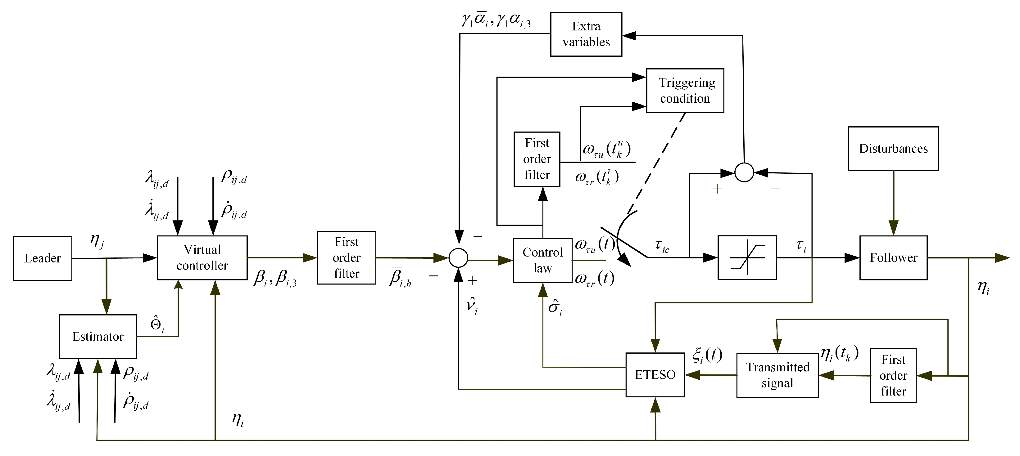
An output feedback controller combined with the ETESO was developed based on an event-triggered strategy. As shown in Figure 3, the characteristic of the proposed controller are as follows. The estimator is used to estimate the velocity of the leader. The ETESO was designed to provide the velocity, yaw rate and uncertainties. The transmitted signal contains an event-triggered strategy that reduces sensor-to-observer communication costs.,The triggering condition of the controller can largely reduce the action times of the actuators. The control law design process is divided into the following steps.

Step 1: Define the formation tracking error vector:

$$\begin{array}{c}\hfill P_{ij}={[{\rho }_{ij,e},{\lambda }_{ij,e}]}^T,\end{array}$$

(49)

where ${\rho }_{ij,e}={\rho }_{ij}-{\rho }_{ij,d}$, and ${\lambda }_{ij,e}={\lambda }_{ij}-{\lambda }_{ij,d}$.

Using (13) and (14), the time derivative of $P_{ij}$ is given as

$$\begin{array}{c}\hfill {\dot{P}}_{ij}=B_{ij}(-{\Xi }_{ij,1}{z}_i+{\Xi }_{ij,2}{z}_j-D_{ij,d}),\end{array}$$

(50)

where $B_{ij}=\mathrm{diag}\{1,\frac{1}{{\rho }_{ij}}\}$,

$${\Xi }_{ij,1}=\left[\begin{array}{cc}\cos ({\psi }_i-{\lambda }_{ij})& -\sin ({\psi }_i-{\lambda }_{ij})\\ \sin ({\psi }_i-{\lambda }_{ij})& \cos ({\psi }_i-{\lambda }_{ij})\end{array}\right],$$

(51)

$${\Xi }_{ij,2}=\left[\begin{array}{cc}\cos ({\psi }_j-{\lambda }_{ij})& -\sin ({\psi }_j-{\lambda }_{ij})\\ \sin ({\psi }_j-{\lambda }_{ij})& \cos ({\psi }_j-{\lambda }_{ij})\end{array}\right],$$

(52)

$z_i={[u_i,v_i]}^T$, $z_j={[u_j,v_j]}^T$ and $D_{ij,d}={[{\dot{\rho }}_{ij,d},{\dot{\lambda }}_{ij,d}]}^T$.

Additionally, $f_i=\left[f_{i,1}{f}_{i,2}\right]=P_{ij}^T{B}_{ij}{\Xi }_{ij,1}$, and $\parallel f_i\parallel \le f_i^{*}$, $f_i^{*}$ is an unknown positive constant.

Remark 3.

The definitions of ${\Xi }_{ij,1}$, $P_{ij}$ and $B_{ij}$, indicate that $\parallel {\Xi }_{ij,1}\parallel =1$, $P_{ij}$ and $B_{ij}$ are bounded, so $\parallel f_i\parallel \le f_i^{*}$ is reasonable.

Choosing ${\beta }_i$ as a virtual controller, ${\beta }_i$ is designed as:

$$\begin{array}{c}\hfill {\beta }_i={\overline{\Xi }}_{ij,1}^{-1}(B_{ij}^{-1}{K}_{i,1}{P}_{ij}+{\widehat{\Theta }}_i-D_{ij,d})+{\overline{f}}_{i,2}\end{array}$$

(53)

where ${\overline{\Xi }}_{ij,1}^{-1}={\Xi }_{ij,1}^T{\left({\Xi }_{ij,1}{\Xi }_{ij,1}^T\right)}^{-1}$, $K_{i,1}\in {\mathbb{R}}^{2\times 2}$ is a positive definite matrix, ${\overline{f}}_{i,2}={[0,\tanh (f_{i,2}/{ϵ}_f)]}^T$, ${ϵ}_f>0$ is a constant, ${\widehat{\Theta }}_i$ is the estimator of ${\Theta }_i$, ${\Theta }_i={\Xi }_{ij,2}{z}_j$ and it updated as

$$\begin{array}{c}\hfill {\dot{\widehat{\Theta }}}_i=-K_{\Theta }{\widehat{\Theta }}_i-{\overline{P}}_{ij},\end{array}$$

(54)

where ${\overline{P}}_{ij}=B_{ij}{[{\rho }_{ij,e}tanh({\rho }_{ij,e}/{ϵ}_{\rho }),{\lambda }_{ij,e}tanh({\lambda }_{ij,e}/{ϵ}_{\lambda })]}^T$, $K_{\Theta }$ is a positive definite matrix, and ${ϵ}_{\rho }$ and ${ϵ}_{\lambda }$ are positive constants.

Remark 4.

The adaptive term ${\widehat{\Theta }}_i$ is employed to reduce the volume of data contained in the formation communication [32] and estimate the information (${\Theta }_i$). ${\Theta }_i$ can be estimated because ${\Xi }_{ij,2}{z}_j\le \left|z_j\right|$, and $z_j$ is bounded, ensuring that formation tracking control is achieved without velocity of the leader and that the amount of data exchanged between USVs can be reduced. Unlike the controller presented in [32], the proposed controller was designed without the velocities of follower. The ETESO can reduce sensor-to-observer communication costs, and the ETC can largely reduce the action times of actuators.

Step 2: An error is defined as

$$\begin{array}{cc}\hfill {\psi }_{i,e}=& {\psi }_i-{\psi }_{ij,a},\hfill \end{array}$$

(55)

where

$$\begin{array}{c}\hfill {\psi }_{ij,a}=[\arctan 2(g_{ij,1},g_{ij,2})-{\psi }_j]\tanh \left(g_{ij,3}\right)+{\psi }_j,\end{array}$$

(56)

where

$$\begin{array}{cc}\hfill g_{ij,1}& ={\rho }_{ij}\sin \left({\lambda }_{ij}\right)-{\rho }_{ij,d}\sin \left({\lambda }_{ij,d}\right),\hfill \end{array}$$

(57)

$$\begin{array}{cc}\hfill g_{ij,2}& ={\rho }_{ij}\cos \left({\lambda }_{ij}\right)-{\rho }_{ij,d}\cos \left({\lambda }_{ij,d}\right),\hfill \end{array}$$

(58)

$$\begin{array}{cc}\hfill g_{ij,3}& =\{{({\rho }_{ij,d}-{\rho }_{ij})}^2+{({\lambda }_{ij,d}-{\lambda }_{ij})}^2\}/{\gamma }_{ij},\hfill \end{array}$$

(59)

where ${\gamma }_{ij}$ is a positive constant.

According to USV dynamics, the time derivative of ${\psi }_{i,e}$ is

$$\begin{array}{c}\hfill {\dot{\psi }}_{i,e}=r_i-{\dot{\psi }}_{ij,a}.\end{array}$$

(60)

The virtual control ${\beta }_{i,3}$ is chosen as:

$$\begin{array}{c}{\beta }_{i,3}=-k_{i,2}{\psi }_{i,e}+{\dot{\psi }}_{ij,a},\hfill \end{array}$$

(61)

where $k_{i,2}$ is a positive constant.

Step 3: Error functions are defined as follows:

$$\begin{array}{cc}\hfill z_{i,e}=& {[u_{i,e},v_{i,e}]}^T={\widehat{z}}_i-{\overline{\beta }}_i-{\gamma }_1{\overline{\alpha }}_i,\hfill \end{array}$$

(62)

$$\begin{array}{cc}\hfill r_{i,e}=& {\widehat{r}}_i-{\overline{\beta }}_{i,3}-{\gamma }_1{\alpha }_{i,3},\hfill \end{array}$$

(63)

$$\begin{array}{cc}\hfill {\omega }_i=& {\overline{\beta }}_i-{\beta }_i,\hfill \end{array}$$

(64)

$$\begin{array}{cc}\hfill {\omega }_{i,3}=& {\overline{\beta }}_{i,3}-{\beta }_{i,3},\hfill \end{array}$$

(65)

where ${\widehat{z}}_i={[{\widehat{u}}_i,{\widehat{v}}_i]}^T$; ${\overline{\beta }}_i={[{\overline{\beta }}_{i,1},{\overline{\beta }}_{i,2}]}^T$; ${\gamma }_1$ is a positive constant; ${\overline{\beta }}_{i,h}$, $h=1,2,3,$ is derived from the first-order filter $l_{i,h}{\dot{\overline{\beta }}}_{i,h}+{\overline{\beta }}_{i,h}={\beta }_{i,h}$; $l_{i,h}>0$ is a constant; ${\overline{\alpha }}_i={[{\alpha }_{i,1},tanh\left({\alpha }_{i,2}\right)/{\gamma }_1]}^T$${\alpha }_{i,h}$, $h=1,2,3,$ is the auxiliary variable derived to deal with the underactuated problem and input saturation. ${\omega }_i={[{\omega }_{i,1},{\omega }_{i,2}]}^T$, ${\omega }_{i,h}$, $h=1,2,3,$ is the error caused by the first order filter.

The updated laws of extra variables are given by

$$\begin{array}{cc}\hfill {\dot{\alpha }}_{i,1}& =\frac{1}{{\gamma }_1}(-T_u{\alpha }_{i,1}-\frac{{\varpi }_{i,u}}{m_{i,11}}),\hfill \end{array}$$

(66)

$$\begin{array}{cc}\hfill {\dot{\alpha }}_{i,2}& =\frac{1}{{cosh}^2\left({\alpha }_{i,2}\right)}({\widehat{\sigma }}_{i,2}+k_{i,4}{v}_{i,e}-f_{i,2}-{\dot{\overline{\beta }}}_{i,2}),\hfill \end{array}$$

(67)

$$\begin{array}{cc}\hfill {\dot{\alpha }}_{i,3}& =\frac{1}{{\gamma }_1}(-T_r{\alpha }_{i,3}-\frac{{\varpi }_{i,r}}{m_{i,33}}),\hfill \end{array}$$

(68)

where $T_u$, $k_{i,4}$ and $T_r$ are positive constants.

Step 4: A control law at the kinetic level is designed as

$$\begin{array}{cc}\hfill {\omega }_{\tau u}\left(t\right)=& m_{i,11}(-k_{i,3}{u}_{i,e}+{\dot{\overline{\beta }}}_{i,1}-T_u{\alpha }_{i,1}+f_{i,1}-{\widehat{\sigma }}_{i,1}),\hfill \end{array}$$

(69)

$$\begin{array}{cc}\hfill {\omega }_{\tau r}\left(t\right)=& m_{i,33}(-k_{i,5}{r}_{i,e}+{\dot{\overline{\beta }}}_{i,3}-T_r{\alpha }_{i,3}-{\psi }_{i,e}-{\widehat{\sigma }}_{i,3}),\hfill \end{array}$$

(70)

where $k_{i,3}$ and $k_{i,5}$ are positive constants.

Remark 5.

In the common continuous control schemes, the controller design has already been completed in Step 4. Here, an event-triggered controller is designed, and the event-triggered condition is be established in the following step. During the flow period between two successive triggering instants, a zero-order holder is used to keep input signals unchanged. The key to a successful ETC design is to choose an appropriate event-triggered strategy. In [23], the triggered condition of a time-varying threshold event-triggered controller (TTETC) is constructed based on flow time and the Lyapunov function. Therefore, the action times of the actuators are limited, and Zeno behavior can be avoided. The signals calculated by controller should be closely related to the triggered condition, its size change determines whether or not to update the control inputs and the change is used to design the proposed triggered condition. It is necessary to provide proof that Zeno behavior is avoided. The appropriate event-triggered strategy reduces the action times of the actuators.

An event-triggeredd controller is chosen as

$$\begin{array}{c}\hfill \begin{array}{c}\hfill \left\{\begin{array}{cc}{\tau }_{i,uc}\left(t\right)={\omega }_{\tau u}\left(t_k^u\right),\hfill & \forall t\in [t_k^u,t_{k+1}^u)\hfill \\ {\tau }_{i,rc}\left(t\right)={\omega }_{\tau r}\left(t_k^r\right),\hfill & \forall t\in [t_k^r,t_{k+1}^r)\hfill \end{array}\right.\end{array}\end{array}$$

(71)

where

$$\begin{array}{c}\hfill \begin{array}{c}\hfill \left\{\begin{array}{cc}{t}_k^u=inf\{t\in \mathbb{R}||e_u\left(t\right)|\ge a_1\},\hfill & t_1^u=0\hfill \\ t_k^r=inf\{t\in \mathbb{R}||e_r\left(t\right)|\ge a_2\},\hfill & t_1^r=0\hfill \\ e_u={\omega }_{\tau u}-{\tau }_{i,uc},e_r={\omega }_{\tau r}-{\tau }_{i,rc},\hfill \end{array}\right.\end{array}\end{array}$$

(72)

and $a_1$ and $a_2$ are positive constants.

The following theorem is provided to demonstrate the stability of the overall closed-loop system.

Theorem 3.

Consider a system consisting of USV dynamics ((7) and (8)), an observer ((15)–(17)), auxiliary variables ((66)–(68)), a control law (71) and environmental disturbances under Assumptions 1–3. Then, the proposed control scheme guarantees that (1) all signals in the closed-loop system are bounded and (2) all USVs can track the leader with a bounded tracking error.

Proof. 

Choose a Lyapunov function candidate as follows:

$$\begin{array}{cc}\hfill V_1=& \frac{1}{2}{P}_{ij}^T{P}_{ij}+\frac{1}{2}{\psi }_{i,e}^2+\frac{1}{2}{u}_{i,e}^2+\frac{1}{2}{v}_{i,e}^2+\frac{1}{2}{r}_{i,e}^2\hfill \\ \hfill & +\frac{1}{2}{\tilde{\Theta }}_i^T{\tilde{\Theta }}_i+\frac{1}{2}\sum _{h=1}^3{\omega }_{i,h}^2+\frac{1}{2}{\alpha }_{i,1}^2+\frac{1}{2}{\alpha }_{i,3}^2,\hfill \end{array}$$

(73)

where ${\tilde{\Theta }}_i={\widehat{\Theta }}_i-{\Theta }_i$.

Along with (50) and (60), the time derivative of $V_1$ is expressed as

$$\begin{array}{cc}\hfill {\dot{V}}_1=& P_{ij}^T{B}_i(-{\Xi }_{ij,1}{z}_i+{\Xi }_{ij,2}{z}_j-D_{ij,d})+{\psi }_{i,e}(r_i-{\dot{\psi }}_{i,a})\hfill \\ \hfill & +u_{i,e}({\dot{\widehat{u}}}_i-{\dot{\overline{\beta }}}_{i,1}-{\gamma }_1{\dot{\alpha }}_{i,1})+v_{i,e}({\dot{\widehat{v}}}_i-{\dot{\overline{\beta }}}_{i,2}-{\dot{\alpha }}_{i,2})\hfill \\ \hfill & +r_{i,e}({\dot{\widehat{r}}}_i-{\dot{\overline{\beta }}}_{i,3}-{\gamma }_1{\dot{\alpha }}_{i,3})+{\tilde{\Theta }}_i^T{\dot{\tilde{\Theta }}}_i+\sum _{h=1}^3{\omega }_{i,h}{\dot{\omega }}_{i,h}\hfill \\ \hfill & +{\alpha }_{i,1}{\dot{\alpha }}_{i,1}+{\alpha }_{i,3}{\dot{\alpha }}_{i,3}.\hfill \end{array}$$

(74)

By applying (21)–(23), (62) and (63) to (74), we obtain

$$\begin{array}{cc}\hfill {\dot{V}}_1=& P_{ij}^T{B}_i[-{\Xi }_{ij,1}(z_{i,e}+{\beta }_i+{\omega }_i+{\gamma }_1{\overline{\alpha }}_i-{\tilde{z}}_i)+{\Xi }_{ij,2}{z}_j\hfill \\ \hfill & -D_{ij,d}]+{\psi }_{i,e}(r_{i,e}+{\beta }_{i,3}+{\omega }_{i,3}+{\gamma }_1{\alpha }_{i,3}-{\tilde{r}}_i\hfill \\ \hfill & -{\dot{\psi }}_{i,a})+u_{i,e}({\zeta }_{i,1}+{\widehat{\sigma }}_{i,1}+\frac{{\tau }_{i,uc}-{\varpi }_{i,u}}{m_{i,11}}-{\dot{\overline{\beta }}}_{i,1}\hfill \\ \hfill & -{\gamma }_1{\dot{\alpha }}_{i,1})+v_{i,e}({\zeta }_{i,2}+{\widehat{\sigma }}_{i,2}-{\dot{\overline{\beta }}}_{i,2}-{\dot{\alpha }}_{i,2})\hfill \\ \hfill & +r_{i,e}({\zeta }_{i,3}+{\widehat{\sigma }}_{i,3}+\frac{{\tau }_{i,rc}-{\varpi }_{i,r}}{m_{i,33}}-{\dot{\overline{\beta }}}_{i,3}-{\gamma }_1{\dot{\alpha }}_{i,3})\hfill \\ \hfill & -{\tilde{\Theta }}_i^T{K}_{\Theta }{\widehat{\Theta }}_i-{\tilde{\Theta }}_i^T{\overline{P}}_{ij}+\sum _{h=1}^3{\omega }_{i,h}{\dot{\omega }}_{i,h}+{\alpha }_{i,1}{\dot{\alpha }}_{i,1}\hfill \\ \hfill & +{\alpha }_{i,3}{\dot{\alpha }}_{i,3}.\hfill \end{array}$$

(75)

Using (53), (54), (61) and (66)–(68) yields

$$\begin{array}{cc}\hfill {\dot{V}}_1=& -P_{ij}^T{K}_{i,1}{P}_{ij}-k_{i,2}{\psi }_{i,e}^2-P_{ij}^T{B}_{ij}{\tilde{\Theta }}_i\hfill \\ \hfill & -f_i(z_{i,e}+{\omega }_i+{\gamma }_1{\overline{\alpha }}_i+{\overline{f}}_{i,2}-{\tilde{z}}_i)\hfill \\ & +{\psi }_{i,e}(r_{i,e}+{\omega }_{i,3}+{\gamma }_1{\alpha }_{i,3}-{\tilde{r}}_i)\hfill \\ \hfill & +u_{i,e}({\zeta }_{i,1}+{\widehat{\sigma }}_{i,1}+\frac{{\tau }_{i,uc}}{m_{i,11}}-{\dot{\overline{\beta }}}_{i,1}+T_u{\alpha }_{i,1})\hfill \\ \hfill & +v_{i,e}(-k_{i,4}{v}_{i,e}+{\zeta }_{i,2}+f_{i,2})\hfill \\ \hfill & +r_{i,e}({\zeta }_{i,3}+{\widehat{\sigma }}_{i,3}+\frac{{\tau }_{i,rc}}{m_{i,33}}-{\dot{\overline{\beta }}}_{i,3}+T_r{\alpha }_{i,3})\hfill \\ \hfill & -{\tilde{\Theta }}_i^T{K}_{\Theta }{\widehat{\Theta }}_i-{\tilde{\Theta }}_i^T{\overline{P}}_{ij}-\sum _{h=1}^3{\omega }_{i,h}(\frac{{\omega }_{i,h}}{l_{i,h}}+{\dot{\beta }}_{i,h})\hfill \\ \hfill & -{\overline{T}}_u{\alpha }_{i,1}^2-{\alpha }_{i,1}{\overline{\varpi }}_{i,u}-{\overline{T}}_r{\alpha }_{i,3}^2-{\alpha }_{i,3}{\overline{\varpi }}_{i,r},\hfill \end{array}$$

(76)

where ${\overline{T}}_u=T_u/{\gamma }_1$, ${\overline{\varpi }}_{i,u}={\varpi }_{i,u}/m_{i,11}$, ${\overline{T}}_r=T_r/{\gamma }_1$ and ${\overline{\varpi }}_{i,r}={\varpi }_{i,r}/m_{i,33}$.

According to (71) and (72), $|{\omega }_{\tau u}-{\tau }_{i,uc}|\le a_1$ and $|{\omega }_{\tau r}-{\tau }_{i,rc}|\le a_2$. There exist time-varying functions (${\mu }_1$, ${\mu }_2$) satisfying $|{\mu }_1|\le 1$ and $|{\mu }_2|\le 1$. Then, ${\omega }_{\tau u}={\tau }_{i,uc}+{\mu }_1{a}_1$ and ${\omega }_{\tau r}={\tau }_{i,rc}+{\mu }_2{a}_2$.

It is worth noting that $f_i{z}_{i,e}=f_{i,1}{u}_{i,e}+f_{i,2}{v}_{i,e}$, and

$$\begin{array}{cc}\hfill -P_{ij}^T{B}_{ij}{\tilde{\Theta }}_i-{\tilde{\Theta }}_i^T{\overline{P}}_{ij}& \le |P_{ij}^T{B}_{ij}{\tilde{\Theta }}_i|-{\tilde{\Theta }}_i^T{\overline{P}}_{ij}\hfill \\ \hfill & \le 0.2758{ϵ}_{\rho }+0.2758{ϵ}_{\lambda }.\hfill \end{array}$$

(77)

Along with (69) and (70), ${\dot{V}}_1$ becomes

$$\begin{array}{cc}\hfill {\dot{V}}_1\le & -P_{ij}^T{K}_{i,1}{P}_{ij}-k_{i,2}{\psi }_{i,e}^2-k_{i,3}{u}_{i,e}^2-k_{i,4}{v}_{i,e}^2\hfill \\ \hfill & -k_{i,5}{r}_{i,e}^2-{\overline{T}}_u{\alpha }_{i,1}^2-{\overline{T}}_r{\alpha }_{i,3}^2-f_i({\omega }_i+{\gamma }_1{\overline{\alpha }}_i\hfill \\ \hfill & +{\overline{f}}_{i,2}-{\tilde{z}}_i)+{\psi }_{i,e}({\omega }_{i,3}+{\gamma }_1{\alpha }_{i,3}-{\tilde{r}}_i)\hfill \\ \hfill & +u_{i,e}({\zeta }_{i,1}-\frac{{\mu }_1{a}_1}{m_{i,11}})+v_{i,e}{\zeta }_{i,2}+r_{i,e}({\zeta }_{i,3}-\frac{{\mu }_2{a}_2}{m_{i,33}})\hfill \\ \hfill & -{\tilde{\Theta }}_i^T{K}_{\Theta }{\widehat{\Theta }}_i+0.2758{ϵ}_{\rho }+0.2758{ϵ}_{\lambda }\hfill \\ \hfill & -\sum _{h=1}^3{\omega }_{i,h}(\frac{{\omega }_{i,h}}{l_{i,h}}+{\dot{\beta }}_{i,h})-{\alpha }_{i,1}{\overline{\varpi }}_{i,u}-{\alpha }_{i,3}{\overline{\varpi }}_{i,r}.\hfill \end{array}$$

(78)

According to Young’s inequality,

$$\begin{array}{cc}\hfill -{\tilde{\Theta }}_i^T{K}_{\Theta }{\widehat{\Theta }}_i\le & -k_{\Theta }{\tilde{\Theta }}_i^T({\tilde{\Theta }}_i+{\Theta }_i)\hfill \\ \hfill & \le \frac{k_{\Theta }}{2}(-{\tilde{\Theta }}_i^T{\tilde{\Theta }}_i+{\Theta }_i^T{\Theta }_i)\hfill \end{array}$$

(79)

where $k_{\Theta }={\lambda }_{min}\left(K_{\Theta }\right)$.

${\dot{V}}_1$ becomes

$$\begin{array}{cc}\hfill {\dot{V}}_1\le & -P_{ij}^T{K}_{i,1}{P}_{ij}-k_{i,2}{\psi }_{i,e}^2-k_{i,3}{u}_{i,e}^2-k_{i,4}{v}_{i,e}^2\hfill \\ \hfill & -k_{i,5}{r}_{i,e}^2-{\overline{T}}_u{\alpha }_{i,1}^2-{\overline{T}}_r{\alpha }_{i,3}^2-\frac{k_{\Theta }}{2}{\tilde{\Theta }}_i^T{\tilde{\Theta }}_i\hfill \\ \hfill & -f_i({\omega }_i+{\gamma }_1{\overline{\alpha }}_i+{\overline{f}}_{i,2}-{\tilde{z}}_i)\hfill \\ \hfill & +{\psi }_{i,e}({\omega }_{i,3}+{\gamma }_1{\alpha }_{i,3}-{\tilde{r}}_i)+u_{i,e}({\zeta }_{i,1}-\frac{{\mu }_1{a}_1}{m_{i,11}})\hfill \\ \hfill & +v_{i,e}{\zeta }_{i,2}+r_{i,e}({\zeta }_{i,3}-\frac{{\mu }_2{a}_2}{m_{i,33}})\hfill \\ \hfill & -\sum _{h=1}^3{\omega }_{i,h}(\frac{{\omega }_{i,h}}{l_{i,h}}+{\dot{\beta }}_{i,h})-{\alpha }_{i,1}{\overline{\varpi }}_{i,u}-{\alpha }_{i,3}{\overline{\varpi }}_{i,r}\hfill \\ \hfill & +\frac{k_{\Theta }}{2}{\Theta }_i^T{\Theta }_i+0.2758{ϵ}_{\rho }+0.2758{ϵ}_{\lambda }.\hfill \end{array}$$

(80)

According to [36] and Young’s inequality,

$$\begin{array}{cc}\hfill -f_i({\gamma }_1{\overline{\alpha }}_{i,1}+{\overline{f}}_{i,2})=& -{\gamma }_1{f}_{i,1}{\alpha }_{i,1}-f_{i,2}tanh\left({\alpha }_{i,2}\right)\hfill \\ \hfill & -\tanh (f_{i,2}/{ϵ}_f)\hfill \\ \hfill & \le \frac{{\gamma }_1^2}{2}{f}_{i,1}^2+\frac{1}{2}{\alpha }_{i,1}^2+0.2785{ϵ}_f.\hfill \end{array}$$

(81)

The following inequalities are used for stability analysis:

$$\begin{array}{cc}\hfill f_i{\tilde{z}}_i=& f_{i,1}{\tilde{u}}_i+f_{i,2}{\tilde{v}}_i\hfill \\ \hfill & \le \frac{1}{2}(f_{i,1}^2+f_{i,2}^2+{\tilde{u}}_i^2+{\tilde{v}}_i^2)\hfill \\ \hfill & \le \frac{1}{2}(f_{i,1}^2+f_{i,2}^2+{ϵ}_i^2{e}_{11}^2+{ϵ}_i^2{e}_{12}^2),\hfill \end{array}$$

(82)

$$\begin{array}{cc}\hfill {\psi }_{i,e}({\gamma }_1{\alpha }_{i,3}-{\tilde{r}}_i)\le & \frac{{\gamma }_1}{2}({\psi }_{i,e}^2+{\alpha }_{i,3}^2)+\frac{1}{2}{\psi }_{i,e}^2+\frac{1}{2}{\tilde{r}}_i^2\hfill \\ \hfill & \le \frac{{\gamma }_1+1}{2}{\psi }_{i,e}^2+\frac{{\gamma }_1}{2}{\alpha }_{i,3}^2+\frac{1}{2}{ϵ}_i^2{e}_{13}^2,\hfill \end{array}$$

(83)

$$\begin{array}{cc}\hfill {\zeta }_{i,1}\le & \frac{3}{{ϵ}_i^2}\left(\right|{\widehat{x}}_i-{\xi }_{i,1}|+|{\widehat{y}}_i-{\xi }_{i,2}\left|\right)\hfill \\ \hfill & \le 3\left(\right|e_{11}|+|q_1|+|e_{12}|+|q_2\left|\right),\hfill \end{array}$$

(84)

$$\begin{array}{cc}\hfill {\zeta }_{i,2}\le & \frac{3}{{ϵ}_i^2}\left(\right|{\widehat{x}}_i-{\xi }_{i,1}|+|{\widehat{y}}_i-{\xi }_{i,2}\left|\right)\hfill \\ \hfill & \le 3\left(\right|e_{11}|+|q_1|+|e_{12}|+|q_2\left|\right),\hfill \end{array}$$

(85)

$$\begin{array}{cc}\hfill {\zeta }_{i,3}\le & \frac{3}{{ϵ}_i^2}\left(\right|{\widehat{\psi }}_i-{\xi }_{i,3}\left|\right)\le 3\left(\right|e_{13}|+|q_3\left|\right),\hfill \end{array}$$

(86)

$$\begin{array}{cc}\hfill u_{i,e}({\zeta }_{i,1}-\frac{{\mu }_1{a}_1}{m_{i,11}})\le & u_{i,e}({\zeta }_{i,1}+{\overline{a}}_1)\hfill \\ \hfill \le & 3u_{i,e}\left(\right|e_{11}|+|q_1|+|e_{12}|+|q_2\left|\right)\hfill \\ \hfill & +|u_{i,e}{\overline{a}}_1|\hfill \\ \hfill \le & \frac{3}{2}(e_{11}^2+q_1^2+e_{12}^2+q_2^2)+\frac{1}{2}{\overline{a}}_1\hfill \\ \hfill & +\frac{13}{2}{u}_{i,e}^2,\hfill \end{array}$$

(87)

$$\begin{array}{cc}\hfill v_{i,e}{\zeta }_{i,2}\le & 3v_{i,e}\left(\right|e_{11}|+|q_1|+|e_{12}|+|q_2\left|\right)\hfill \\ \hfill & \le \frac{3}{2}(e_{11}^2+q_1^2+e_{12}^2+q_2^2)+6v_{i,e}^2,\hfill \end{array}$$

(88)

$$\begin{array}{cc}\hfill r_{i,e}({\zeta }_{i,3}-\frac{{\mu }_2{a}_2}{m_{i,33}})\le & r_{i,e}({\zeta }_{i,3}+{\overline{a}}_2)\hfill \\ \hfill \le & 3r_{i,e}\left(\right|e_{13}|+|q_3\left|\right)+|r_{i,e}{\overline{a}}_2|\hfill \\ \hfill \le & \frac{3}{2}(e_{13}^2+q_3^2)+\frac{7}{2}{r}_{i,e}^2+\frac{1}{2}{\overline{a}}_2^2,\hfill \end{array}$$

(89)

$$\begin{array}{c}\hfill {\alpha }_{i,1}{\overline{\varpi }}_{i,u}\le \frac{1}{2}{\alpha }_{i,1}^2+\frac{1}{2}{\overline{\varpi }}_{i,u}^2,\end{array}$$

(90)

$$\begin{array}{c}\hfill {\alpha }_{i,3}{\overline{\varpi }}_{i,r}\le \frac{1}{2}{\alpha }_{i,3}^2+\frac{1}{2}{\overline{\varpi }}_{i,r}^2,\end{array}$$

(91)

where ${\overline{a}}_1=a_1/m_{i,11}$, and ${\overline{a}}_2=a_2/m_{i,33}$.

Then, the following inequality can be obtained:

$$\begin{array}{cc}\hfill {\dot{V}}_1\le & -P_{ij}^T{K}_{i,1}{P}_{ij}-(k_{i,2}-{\overline{\gamma }}_1){\psi }_{i,e}^2-(k_{i,3}-\frac{13}{2})u_{i,e}^2\hfill \\ \hfill & -(k_{i,4}-6)v_{i,e}^2-(k_{i,5}-\frac{7}{2})r_{i,e}^2-\frac{k_{\Theta }}{2}{\tilde{\Theta }}_i^T{\tilde{\Theta }}_i\hfill \\ \hfill & -({\overline{T}}_u-\frac{1}{2}){\alpha }_{i,1}^2-({\overline{T}}_r-{\overline{\gamma }}_1){\alpha }_{i,3}^2-f_i{\omega }_i\hfill \\ \hfill & +{\psi }_{i,e}{\omega }_{i,3}-\sum _{h=1}^3{\omega }_{i,h}(\frac{{\omega }_{i,h}}{l_{i,h}}+{\dot{\beta }}_{i,h})+\frac{{ϵ}_i^2+6}{2}{e}_{11}^2\hfill \\ \hfill & +\frac{{ϵ}_i^2+6}{2}{e}_{12}^2+\frac{{ϵ}_i^2+3}{2}{e}_{13}^2+c_1,\hfill \end{array}$$

(92)

where ${\overline{\gamma }}_1=\frac{{\gamma }_1+1}{2}$, and $c_1=\frac{k_{\Theta }}{2}{\Theta }_i^T{\Theta }_i+0.2758{ϵ}_{\rho }+0.2758{ϵ}_{\lambda }+\frac{{\gamma }_1^2}{2}{f}_{i,1}^2+0.2785{ϵ}_f+\frac{1}{2}(f_{i,1}^2+f_{i,2}^2)+\frac{1}{2}{\overline{\varpi }}_{i,u}^2+\frac{1}{2}{\overline{\varpi }}_{i,r}^2+3(q_1^2+q_2^2+\frac{1}{2}{q}_3^2)+\frac{1}{2}{\overline{a}}_1+\frac{1}{2}{\overline{a}}_2$.

Consider the total Lyapunov function as

$$\begin{array}{c}\hfill V_2=V_1+V_o,\end{array}$$

(93)

□

Remark 6.

The Lyapunov function ($V_1$) includes estimation errors ($e_{11}$, $e_{12}$, $e_{13}$). We cannot conclude that ${\dot{V}}_1\le -c_0{V}_1+c_3$, $c_0$ and $c_3$ are positive constants. The Lyapunov function ($V_2$) is constructed by inducing $V_o$. In the time derivative of $V_2$, the gain of estimation error is negative. We can conclude that ${\dot{V}}_2\le -c_0{V}_2+c_3$. Therefore, it is proven that all signals of the closed-loop system are bounded.

Along with (48) and (92), the time derivative of $V_2$ is

$$\begin{array}{cc}\hfill {\dot{V}}_2\le & -P_{ij}^T{K}_{i,1}{P}_{ij}-(k_{i,2}-{\overline{\gamma }}_1){\psi }_{i,e}^2-(k_{i,3}-\frac{13}{2})u_{i,e}^2\hfill \\ \hfill & -(k_{i,4}-6)v_{i,e}^2-(k_{i,5}-\frac{7}{2})r_{i,e}^2-\frac{k_{\Theta }}{2}{\tilde{\Theta }}_i^T{\tilde{\Theta }}_i\hfill \\ \hfill & -({\overline{T}}_u--\frac{1}{2}){\alpha }_{i,1}^2-({\overline{T}}_r-{\overline{\gamma }}_1){\alpha }_{i,3}^2-f_i{\omega }_i\hfill \\ \hfill & +{\psi }_{i,e}{\omega }_{i,3}-\sum _{h=1}^3{\omega }_{i,h}(\frac{{\omega }_{i,h}}{l_{i,h}}+{\dot{\beta }}_{i,h})\hfill \\ \hfill & -c_2{\parallel E_t\left(t\right)\parallel }^2+c_1,\hfill \end{array}$$

(94)

where $c_2=\frac{\varrho (1-c_{o_1})}{2}-\frac{{ϵ}_i^2+6}{2}$.

Define ${\Omega }_{i,1}=-f_{i,1}-{\dot{\beta }}_{i,1}$, ${\Omega }_{i,2}=-f_{i,2}-{\dot{\beta }}_{i,2}$ and ${\Omega }_{i,3}={\psi }_{i,e}-{\dot{\beta }}_{i,3}$. According to Young’s inequality, ${\omega }_{i,h}{\Omega }_{i,h}$$\le \frac{1}{2{\varrho }_c}{\omega }_{i,h}^2{\Omega }_{i,h}^2+\frac{{\varrho }_c}{2}$. Then,

$$\begin{array}{cc}\hfill {\dot{V}}_2\le & -P_{ij}^T{K}_{i,1}{P}_{ij}-(k_{i,2}-{\overline{\gamma }}_1){\psi }_{i,e}^2-(k_{i,3}-\frac{13}{2})u_{i,e}^2\hfill \\ \hfill & -(k_{i,4}-6)v_{i,e}^2-(k_{i,5}-\frac{7}{2})r_{i,e}^2-\frac{k_{\Theta }}{2}{\tilde{\Theta }}_i^T{\tilde{\Theta }}_i\hfill \\ \hfill & -({\overline{T}}_u-\frac{1}{2}){\alpha }_{i,1}^2-({\overline{T}}_r-{\overline{\gamma }}_1){\alpha }_{i,3}^2\hfill \\ \hfill & -\sum _{h=1}^3(\frac{{\omega }_{i,h}^2}{l_{i,h}}-\frac{{\omega }_{i,h}^2{\Omega }_{i,h}^2}{2{\varrho }_c})-c_2{\parallel E_t\left(t\right)\parallel }^2+c_3,\hfill \end{array}$$

(95)

where $c_3=c_1+\frac{3}{2}{\varrho }_c$, ${\varrho }_c$ is a positive constant.

$|{\Omega }_{i,h}|\le s_{i,h}$, $s_{i,h}$, $h=1,2,3$ is a positive constant. $\frac{1}{l_{i,h}}=s_{i,h}^2/\left(2{\varrho }_c\right)+l_{i,h}^{*}$ with $l_{i,h}^{*}>0$ is a constant. The follow can be attained:

$$\begin{array}{cc}\hfill {\dot{V}}_2\le & -P_{ij}^T{K}_{i,1}{P}_{ij}-(k_{i,2}-{\overline{\gamma }}_1){\psi }_{i,e}^2-(k_{i,3}-\frac{13}{2})u_{i,e}^2\hfill \\ \hfill & -(k_{i,4}-6)v_{i,e}^2-(k_{i,5}-\frac{7}{2})r_{i,e}^2-\frac{k_{\Theta }}{2}{\tilde{\Theta }}_i^T{\tilde{\Theta }}_i\hfill \\ \hfill & -({\overline{T}}_u-\frac{1}{2}){\alpha }_{i,1}^2-({\overline{T}}_r-{\overline{\gamma }}_1){\alpha }_{i,3}^2\hfill \\ \hfill & -\sum _{h=1}^3{l}_{i,h}^{*}{\omega }_{i,h}^2-\sum _{h=1}^3(1-\frac{{\Omega }_{i,h}^2}{s_{i,h}^2})\frac{{\omega }_{i,h}^2{s}_{i,h}^2}{2{\varrho }_i}\hfill \\ \hfill & -c_2{\parallel E_t\left(t\right)\parallel }^2+c_3,\hfill \end{array}$$

(96)

Owing to $|{\Omega }_{i,h}|\le s_{i,h}$, the inequality (96) becomes

$$\begin{array}{c}\hfill {\dot{V}}_2\le -c_0{V}_2+c_3,\end{array}$$

(97)

where $c_0=\min \{2{\lambda }_{min}\left(K_{i,1}\right),2(k_{i,2}-{\overline{\gamma }}_1),2(k_{i,3}-\frac{13}{2}),2(k_{i,4}-6),2(k_{i,5}-\frac{7}{2})$, $k_{\Theta }$, $2({\overline{T}}_u-\frac{1}{2})$, $2({\overline{T}}_r-{\overline{\gamma }}_1)$, $2l_{i,h}^{*}$, $2c_2/{\lambda }_{max}\left(P\right)\}$.

Theorem 4.

Zeno behavior can be avoided under the event-triggered mechanisms ((71) and (72)), and the implementation intervals $t_{k+1}^u-t_k^u$ and $t_{k+1}^r-t_k^r$ are lower-bounded by a positive constant ($t^{*}$).

Proof. 

According to (72),

$$\begin{array}{c}\hfill \begin{array}{c}\hfill \left\{\begin{array}{cc}\frac{d}{dt}|e_u|=\mathrm{sign}\left(e_u\right){\dot{e}}_u\le \left|{\dot{\omega }}_{\tau u}\right|,\hfill & \forall t\in [t_k^u,t_{k+1}^u)\hfill \\ \frac{d}{dt}|e_r|=\mathrm{sign}\left(e_r\right){\dot{e}}_r\le \left|{\dot{\omega }}_{\tau r}\right|.\hfill & \forall t\in [t_k^r,t_{k+1}^r)\hfill \end{array}\right.\end{array}\end{array}$$

(98)

The time derivatives of ${\omega }_{\tau u}$ and ${\omega }_{\tau r}$ are expressed as

$$\begin{array}{cc}\hfill {\dot{\omega }}_{\tau u}\left(t\right)=& m_{i,11}(-k_{i,3}{\dot{u}}_{i,e}+{\ddot{\overline{\beta }}}_{i,1}-T_u{\dot{\alpha }}_{i,1}+{\dot{f}}_{i,1}-{\dot{\widehat{\sigma }}}_{i,1}),\hfill \end{array}$$

(99)

$$\begin{array}{cc}\hfill {\dot{\omega }}_{\tau r}\left(t\right)=& m_{i,33}(-k_{i,5}{\dot{r}}_{i,e}+{\ddot{\overline{\beta }}}_{i,3}-T_r{\dot{\alpha }}_{i,3}-{\dot{\psi }}_{i,e}-{\dot{\widehat{\sigma }}}_{i,3}).\hfill \end{array}$$

(100)

□

Theorem 3 shows that all signals in the closed-loop system are bounded. Therefore, ${\dot{u}}_{i,e},{\dot{r}}_{i,e},{\ddot{\overline{\beta }}}_{i,1},{\ddot{\overline{\beta }}}_{i,3},{\dot{\alpha }}_{i,1},{\dot{\alpha }}_{i,3}$ and ${\dot{\psi }}_{i,e}$ are bounded. According to the design of the ETESO, ${\dot{\widehat{\sigma }}}_{i,1}$ and ${\dot{\widehat{\sigma }}}_{i,3}$ are bounded. ${\dot{f}}_{i,1}$ is bounded because $\parallel f_i\parallel \le f_i^{*}$. Therefore, there are positive constants ($k_u$ and $k_r$) satisfying $|{\dot{\omega }}_{\tau u}|\le k_u$ and $|{\dot{\omega }}_{\tau r}|\le k_r$. Since

$$\begin{array}{c}\hfill \begin{array}{c}\hfill \left\{\begin{array}{cc}{e}_u\left(t_k^u\right)=0,\hfill & limt\to t_{k+1}^u\left|e_u\left(t\right)\right|=a_1\hfill \\ e_r\left(t_k^r\right)=0,\hfill & limt\to t_{k+1}^r\left|e_r\left(t\right)\right|=a_2\hfill \end{array}\right.\end{array}\end{array}$$

(101)

there exists a lower bound of implementation interval $t^{*}$ and $t^{*}\ge min\{a_1/k_u,a_2/k_r\}$. Hence, no Zeno phenomenon occurs when the proposed control law is used.

5. Simulation Results

In this section, simulation results are presented to prove the proposed event-triggered control method, and the ship parameters are chosen from [37]. Four USVs were driven to track a leader at a desired distance and angle with the proposed control law in (69)–(72). The total duration of the simulation runs was 120 s, and the sampling time $t_s$ for each time point was $0.01$ s. The initial positions of followers were chosen as ${\eta }_1\left(0\right)=[-2$ m, $-5$ m, 0 rad${]}^T$, ${\eta }_2\left(0\right)=[-2$ m, 5 m, 0 rad${]}^T$, ${\eta }_3\left(0\right)=[-4$ m, $-8$ m, 0 rad${]}^T$ and ${\eta }_4\left(0\right)=[-4$ m, 8 m, 0 rad${]}^T$. The trajectory of leader was generated by $u_j=0.2$ m/s, $v_j=0$ m/s and $r_j=0$ rad/s for $0\le t<40$ s; $u_j=0.2$ m/s, $v_j=0$ m/s and $r_j=0.1$ rad/s for 40 s$\le t<60$ s; $u_j=0.2$ m/s, $v_j=0$ m/s and $r_j=-0.1$ rad/s for 60 s$\le t<80$ s, $u_j=0.2$ m/s, $v_j=0$ m/s and $r_j=0$ rad/s for 80 s$\le t<120$ s; and ${\eta }_j\left(0\right)=[0$ m, 0 m, 0 rad${]}^T$. The desired distance and relative angle are expressed by ${\rho }_{1j,d}=3$ m, ${\lambda }_{1j,d}=1$ rad, ${\rho }_{2j,d}=3$ m, ${\lambda }_{2j,d}=-1$ rad, ${\rho }_{3j,d}=6$ m, ${\lambda }_{3j,d}=1$ rad, ${\rho }_{4j,d}=6$ m and ${\lambda }_{4j,d}=-1$ rad.

The parameters of the ETESO were chosen as ${ϵ}_i=0.4$, $c_q=0.1$. The parameters of the proposed control law were chosen as ${ϵ}_f=0.1$, $K_{\Theta }=\mathrm{diag}\{5,5\}$, ${\gamma }_{ij}=0.001$, $K_{i,1}=\mathrm{diag}\{5,5\}$, $k_{i,2}=5,$$k_{i,3}=10$, $k_{i,4}=10$, $k_{i,5}=10$, ${\gamma }_1=5$, $T_u=10$, $T_r=16$, $l_{i,h}=0.1$ and $h=1,2,3$. The parameters of the trigger condition were $a_1=a_2=0.2$.

Remark 7.

According to inequality (97), we should keep $c_0$ as large as possible and $c_3$ as small as possible. A closed-loop system can converge quickly with small errors. However, $c_3$ includes the mismatch variables between input without saturation and input with saturation (${\overline{\varpi }}_{i,u}$ and ${\overline{\varpi }}_{i,r}$). Large gain factors ($K_{i,1}$, $k_{i,2}$, $k_{i,3}$, $k_{i,4}$ and $k_{i,5}$) correspond to large mismatch variables. Therefore, gain factor was set as small as possible without violating the $c_0>0$ constraint. ${\gamma }_1$, $T_u$ and $T_r$ define the convergence rate of auxiliary variables and satisfy the inequalities $T_u/{\gamma }_1-1/2>0$ and $T_r/{\gamma }_1-(1+{\gamma }_1)/2>0$. $l_{i,h}$ determines the tracking speed of the first-order filter, which is related to the sampling time of the simulation. An excessively large value results in an unstable system, and an excessively small value results in poor tracking performance. As a rule of thumb, the general recommended value of $l_{i,h}$ is between $t_s$ and $10t_s$. The parameters $a_1$ and $a_2$ define the trigger condition of the proposed controller; larger $a_1$ and $a_2$ values indicate a lower update frequency of input signals and a poor system performance. To find a balance between update frequency and system performance, $a_1$ and $a_2$ are defined as $a_1=a_2=0.2$. ${ϵ}_i$ defines the estimation speed of the ETESO, $c_q$ is the threshold of the trigger condition of the ETESO and the process of parameter selection is similar to parameter selection in $a_1$ and $a_2$. The ETESO and feed-forward compensation are relied upon, the influence of uncertainties is compensated immediately and the closed-loop system possesses strong robustness to different sets of parameters.

For surface vessels, the effect of gravity can be neglected because the gravity acting on USVs is equal to the buoyancy acting on USVs. USVs are subject to model uncertainties and environmental disturbances. Model uncertainties are induced by model errors and unknown system parameters. Therefore, only centrifugal terms, damping parameters and environmental disturbances are considered. In this paper, the uncertainties ${\sigma }_{i,1}$, ${\sigma }_{i,2}$ and ${\sigma }_{i,3}$ are assumed to be unknown. Environmental disturbances contain wind, wave and current information. The impacts on USVs of wind can be ignored due to a small windward area. Therefore, environmental disturbances are designed as the sum of some sinusoidal signals, which are chosen as $[0.18-0.18\cos (0.01t\left)\cos \right(0.015t),0.6+0.18\sin (0.21t\left)\cos \right(0.2t),$${0.6-0.18\sin \left(0.2t\right)\cos \left(0.23t\right)]}^T$.

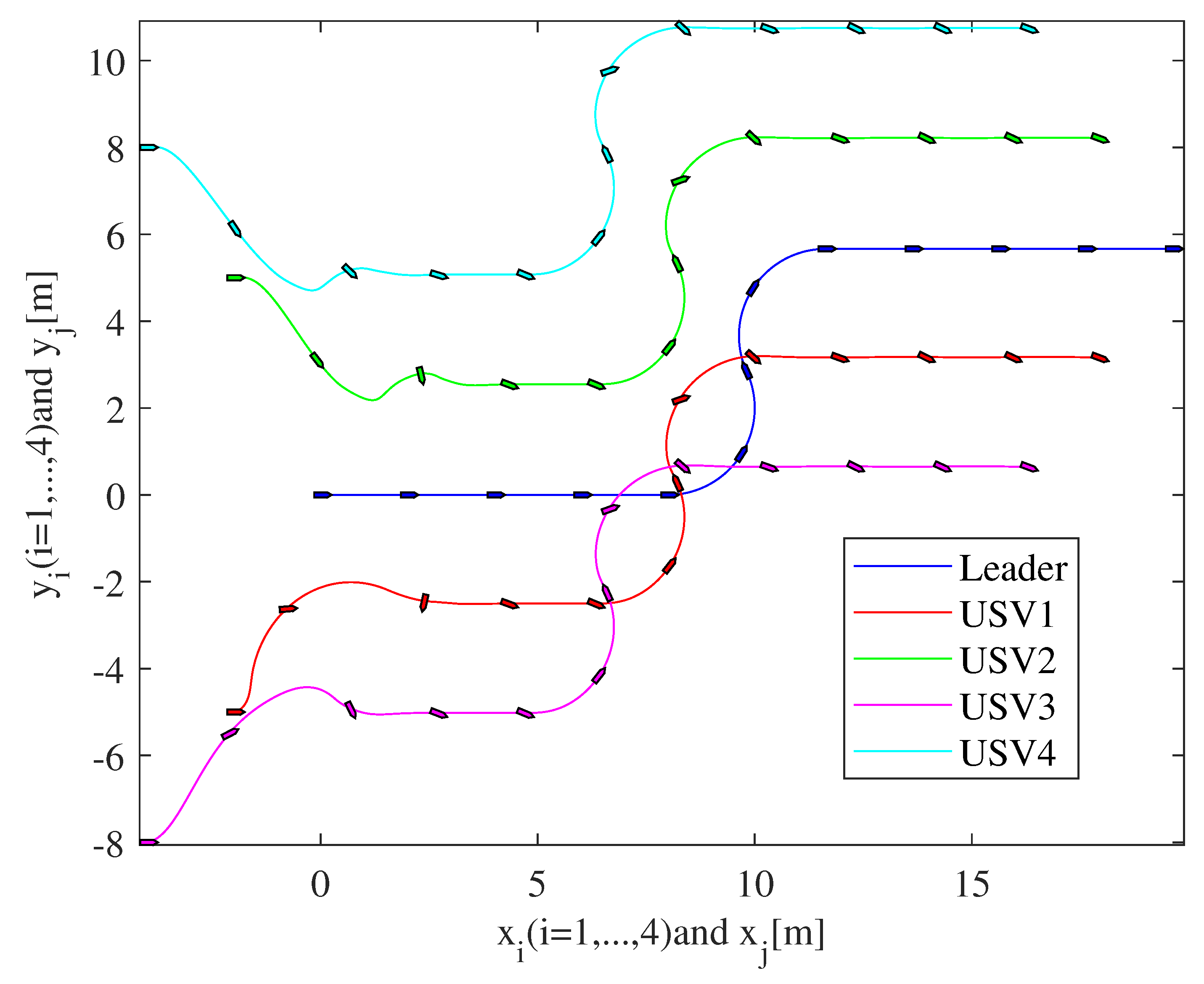
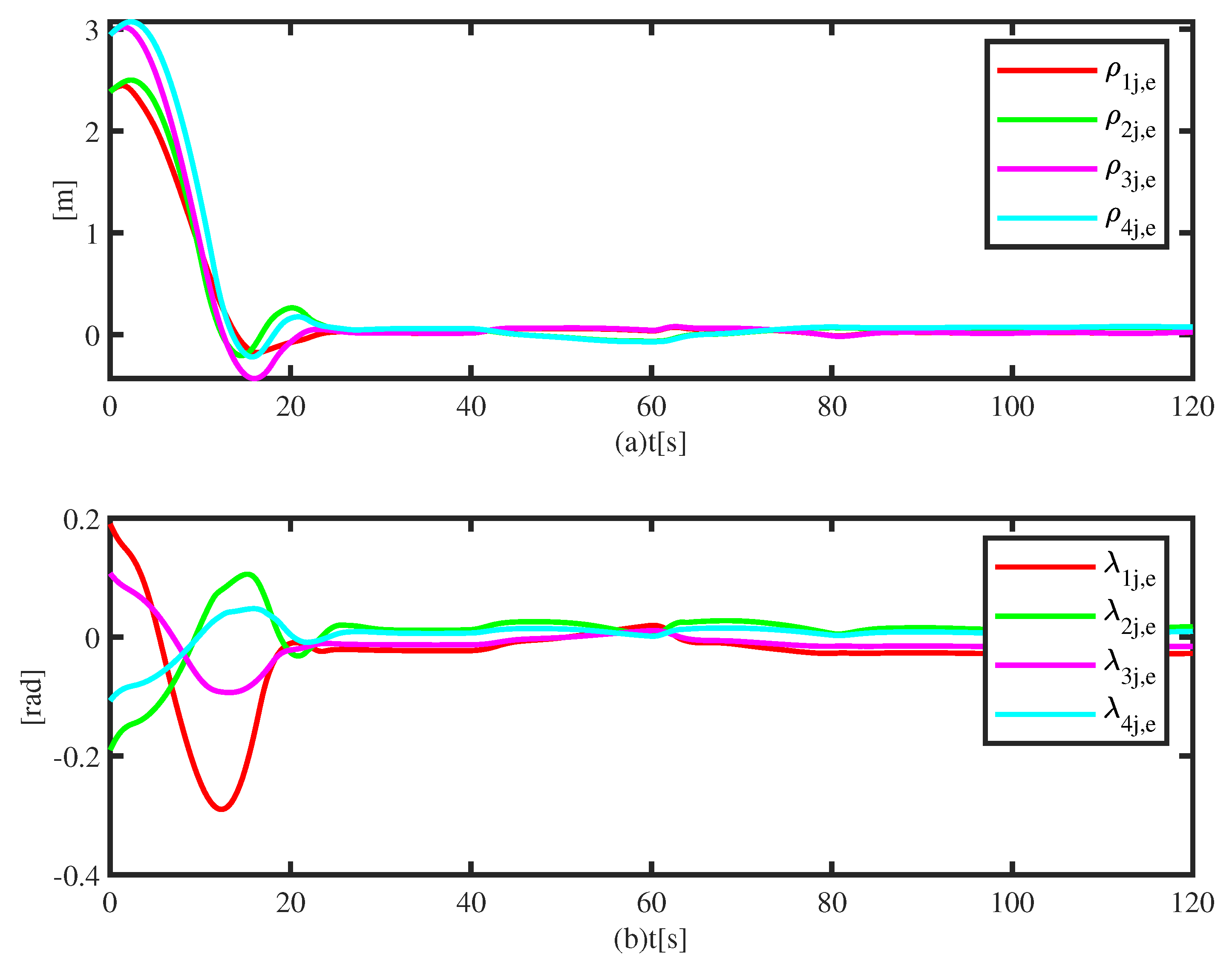
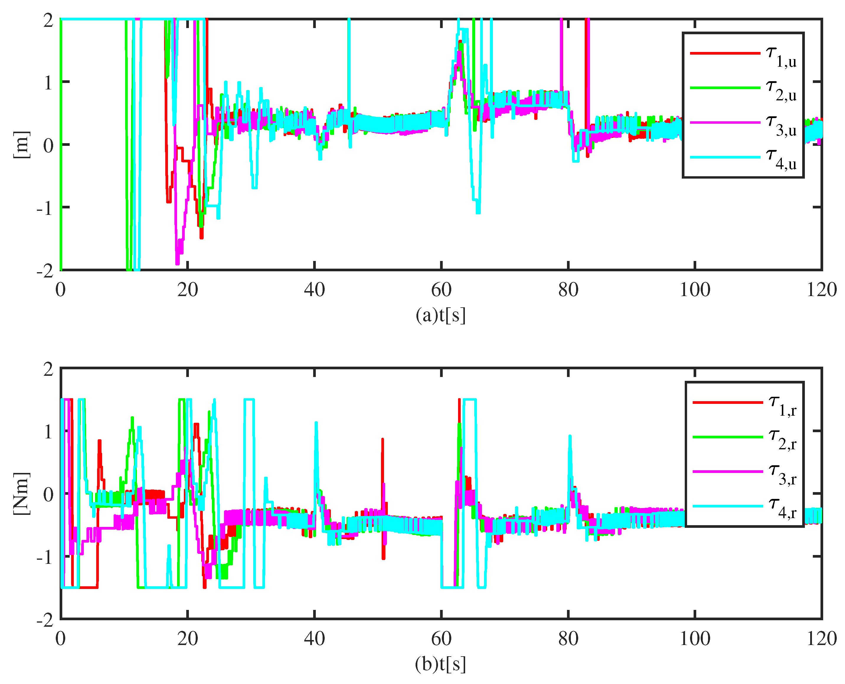
Simulation results are shown in Figure 4, Figure 5, Figure 6, Figure 7, Figure 8 and Figure 9. Figure 4 shows the formation pattern shaped by the five vessels; all followers can successfully track the leader. Figure 5 shows that the formation tracking errors approach zero, regardless of model uncertainties and environmental disturbances. Figure 6 shows the input signals of four USVs. In the first 24 s, since initial formation tracking errors are large, saturated control inputs suffer from sudden jumps. From 25 s to 40 s, formation tracking errors approach zero, and input signals convergence gradually. At 40s, 60s and 80s, sudden changes in the control forces are caused by a sudden change of the leader’s velocity.

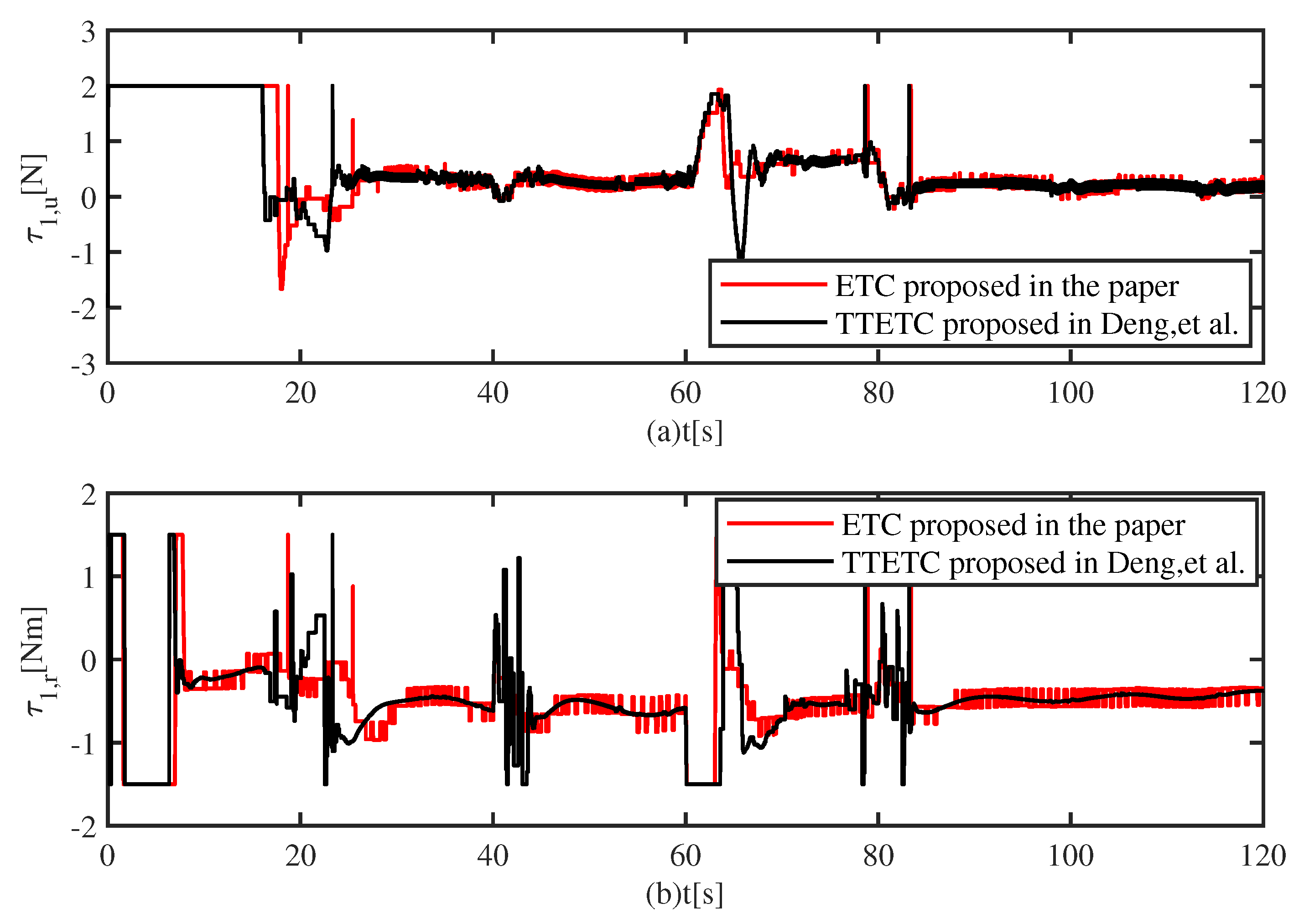
Comparisons of simulation results are shown in Figure 7, Figure 8 and Figure 9. Simulations were conducted using the TTETC proposed in [23] and the ETC proposed in this paper. The two controllers have same control parameters but different trigger condition parameters.

The TTETC was designed as follows:

$$\begin{array}{c}\hfill \begin{array}{c}\hfill \left\{\begin{array}{cc}{\tau }_{i,uc}\left(t\right)={\omega }_{\tau u}\left(t_k^u\right),\hfill & \forall t\in [t_k^u,t_{k+1}^u)\hfill \\ {\tau }_{i,rc}\left(t\right)={\omega }_{\tau r}\left(t_k^r\right),\hfill & \forall t\in [t_k^r,t_{k+1}^r)\hfill \end{array}\right.\end{array}\end{array}$$

(102)

with

$$\begin{array}{c}\hfill \begin{array}{c}\hfill \left\{\begin{array}{cc}{t}_k^u=inf\{t\in \mathbb{R}|t>t_{k-1}^u\wedge e_u>\sigma V_2\wedge V_2>\mu \},\hfill & t_1^u=0\hfill \\ t_k^r=inf\{t\in \mathbb{R}|t>t_{k-1}^r\wedge e_r>(1-\sigma )V_2\wedge V_2>\mu \},\hfill & t_1^r=0\hfill \\ e_u={\omega }_{\tau u}-{\tau }_{i,uc},e_r={\omega }_{\tau r}-{\tau }_{i,rc},\hfill \end{array}\right.\end{array}\end{array}$$

(103)

$\mu =0.02$, $\sigma =0.5$.

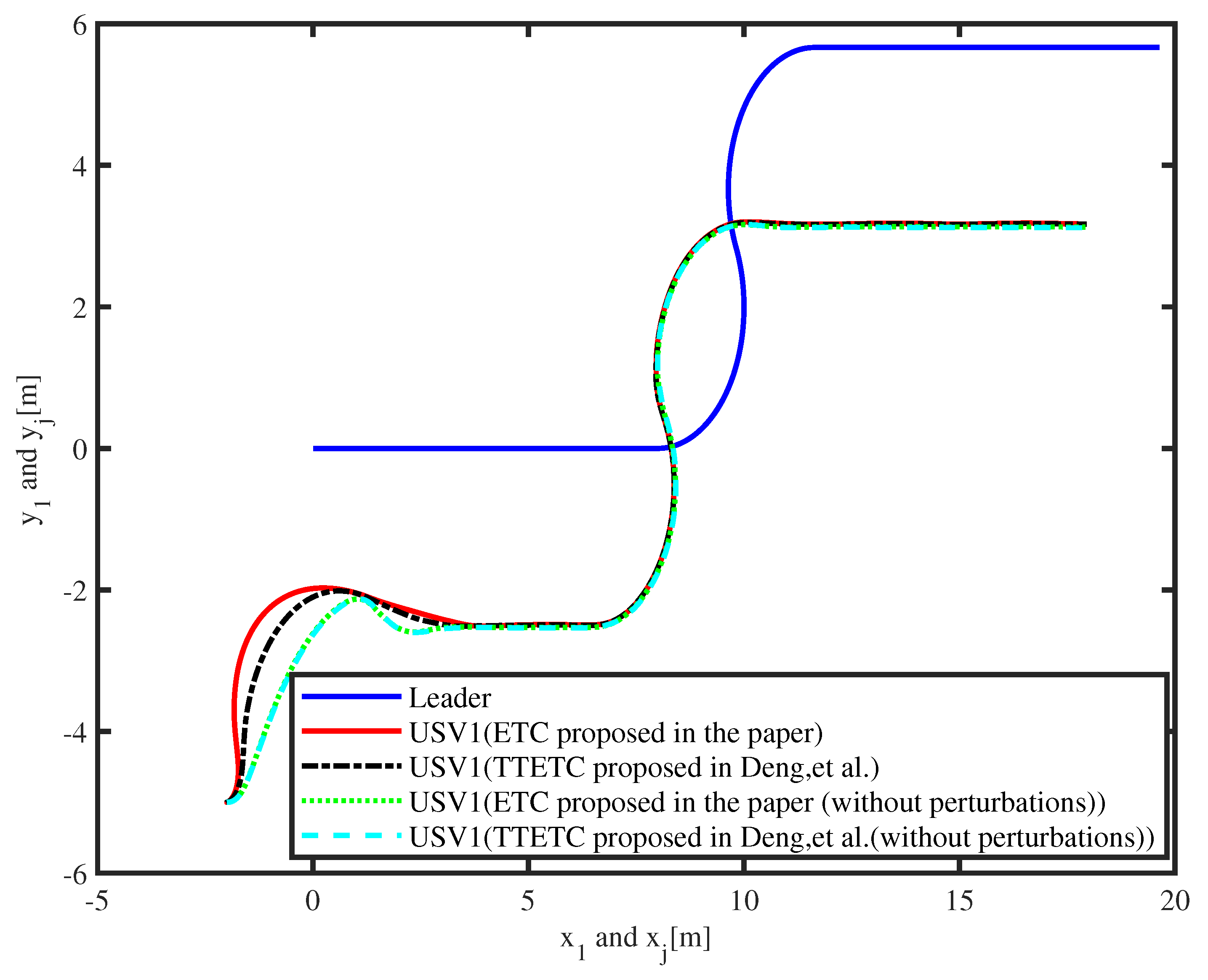
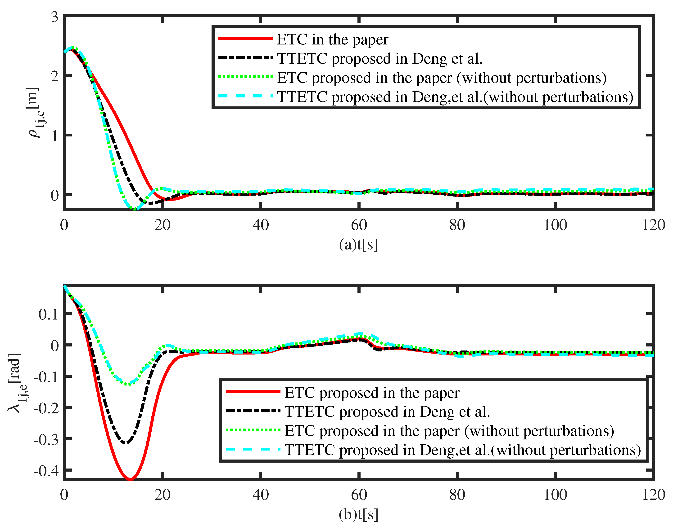
Figure 7 depicts a formation pattern shaped by the ith USV and the leader. Different controllers are applied to the system with and without perturbations, revealing that the follower is able to track the leader successfully under four different conditions. Figure 8 depicts the distance and angle tracking errors under four different conditions, showing that the errors converge to the small neighborhood of the origin. Compared with the system with perturbations, the system without perturbations has a faster convergence rate. In the system with perturbations, some control energy is used to reject disturbances, including model uncertainties and environmental disturbances. Then, the energy that causes the system to converge is reduced. Under the same condition, the stability errors and convergence rates of the TTETC and ETC are nearly the same. The two controllers have the same structure but different event-triggered strategies. Therefore, they have the same convergence rate but different action times of the actuators. Figure 9 depicts the control signals generated by each of the controllers. Due to the effect of the proposed controller, the input signals shake at low frequencies, but their amplitudes are higher. At the beginning, due to a large initial formation tracking error, the input signals are saturated. The input signals converge, along with the convergence of formation tracking error. At 40 s, 60 s and 80 s, the input signals shake due to changes in the velocity of the leader. 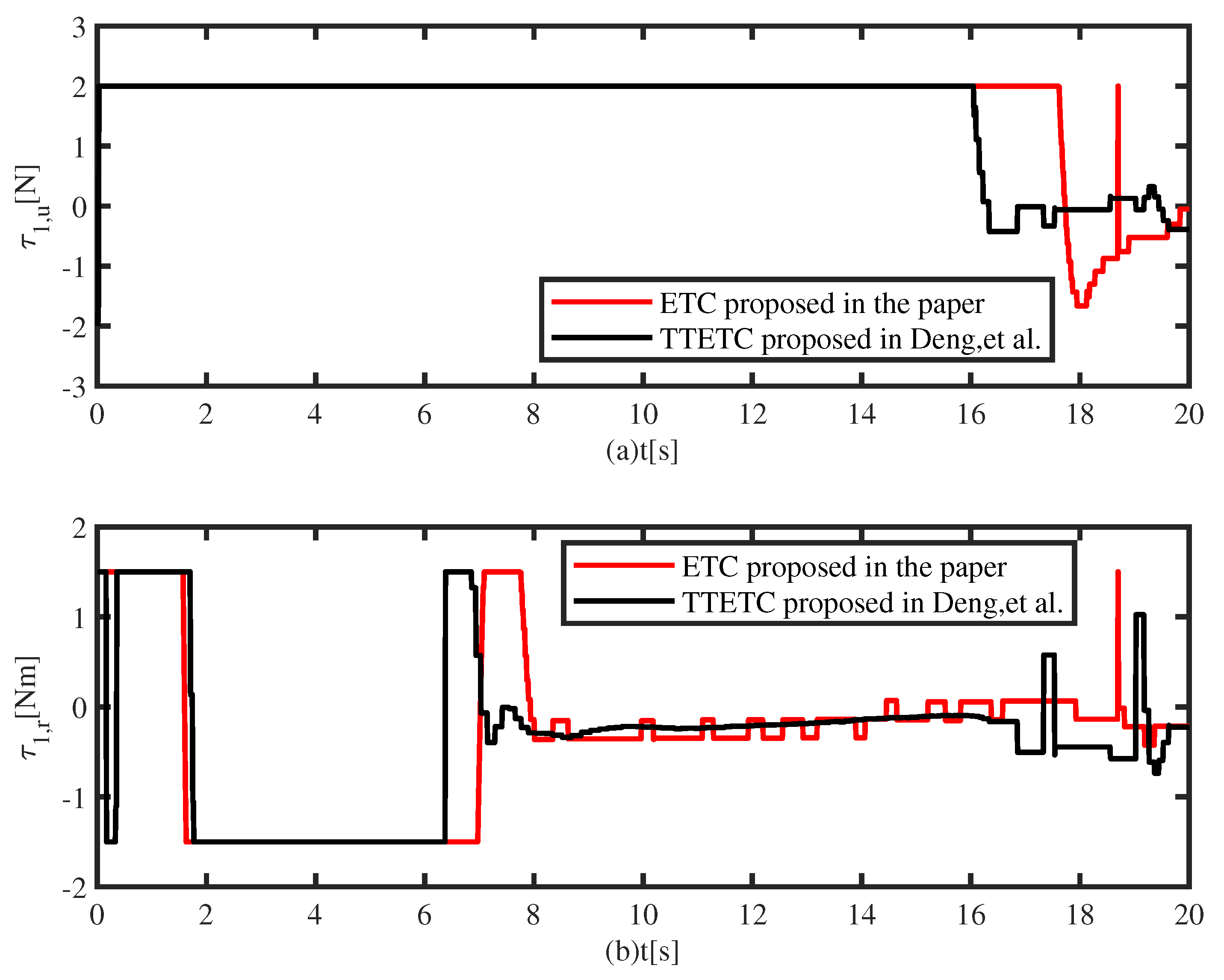Figure 10 shows the control inputs within the first 20 s; the update frequencies of control inputs differ due to differing triggering strategies.

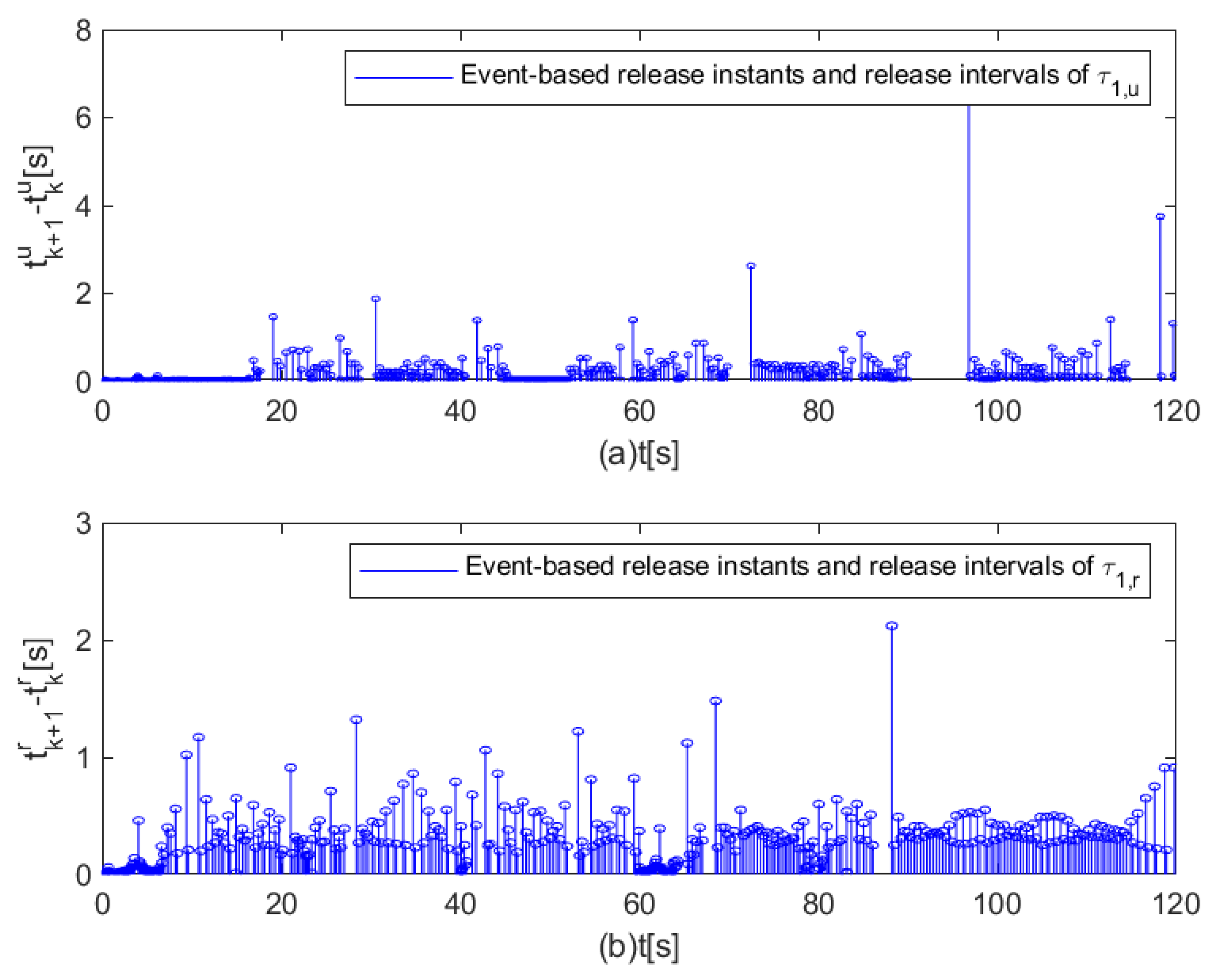
Figure 11 shows the event-based release instants and release intervals of input signals under the proposed controller. As shown in

Table 2. Comparisons of ETC and TTETC.

Performance Parameter	ETC	TTETC
Convergent time	24.25 s	24.26 s
Convergent time (without perturbations)	24.21 s	24.22 s
Stability error ${\rho }_{1j,e}$	0.01 m	0.01 m
Stability error ${\rho }_{1j,e}$ (without perturbations)	0.01 m	0.01 m
Stability error ${\lambda }_{1j,e}$	−0.02 rad	−0.02 rad
Stability error ${\lambda }_{1j,e}$ (without perturbations)	−0.01 rad	−0.01 rad
Action times of ${\tau }_{1,uc}$	1321	2226
Action times of ${\tau }_{1,uc}$ (without perturbations)	1210	2064
Action times of ${\tau }_{1,rc}$	702	2226
Action times of ${\tau }_{1,rc}$ (without perturbations)	504	2064

, compared with the TTETC, the proposed ETC largely reduces the action times of the actuators. The triggering condition of the TTETC was designed based on the Lyapunov function ($V_2$). In order to ensure the performance of control systems, the threshold is set to a smaller value. The threshold of the ETC was set to $0.2$, and the action times of the actuators can be largely reduced.

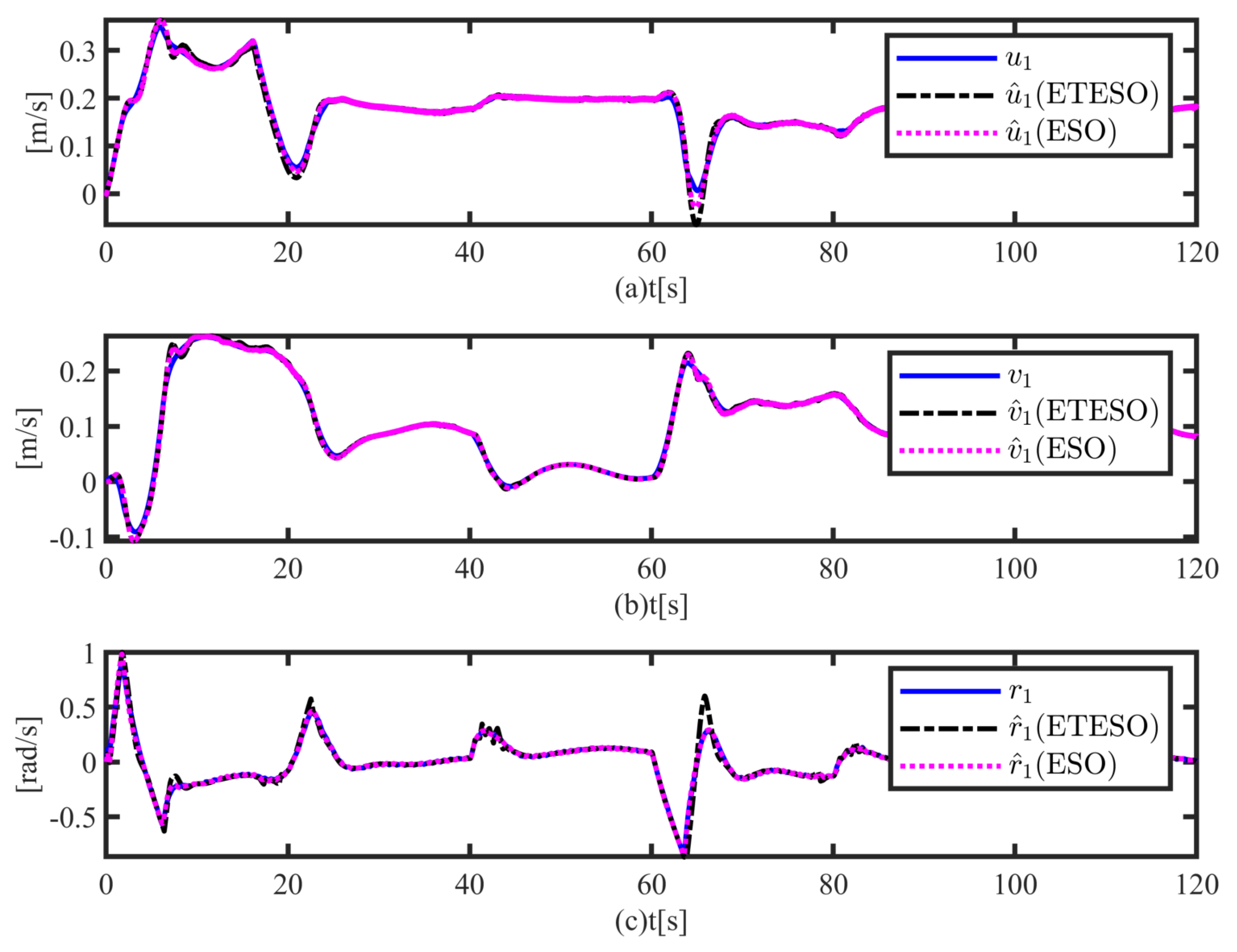
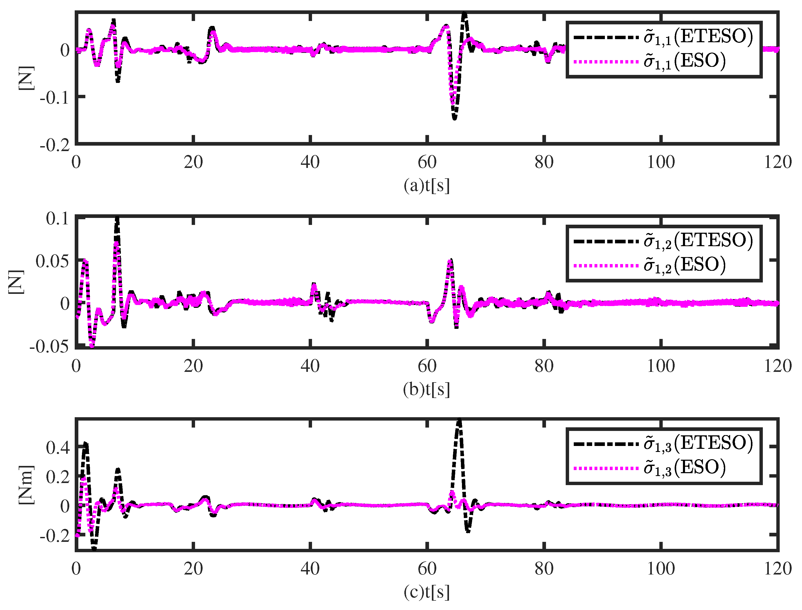
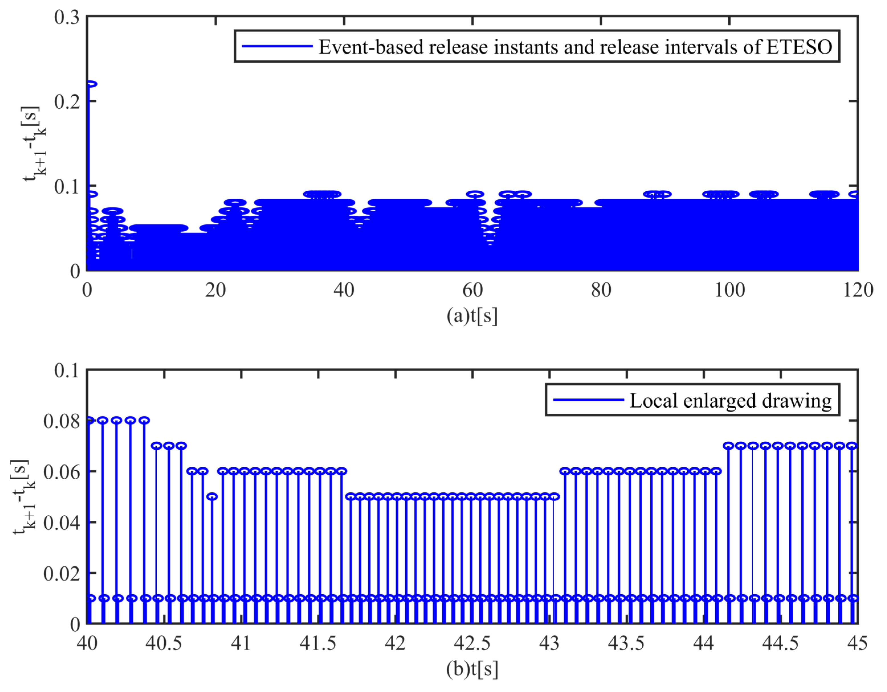
The ESO was proposed in [31]. Figure 12 shows the estimated velocities and real velocities, illustrating that the velocity estimation of the ETESO is as good as that of the ESO. Figure 13 shows that the uncertainties are effectively approximated by the ESO and ETESO. Compared to the ESO, the ETESO simultaneously obtains a large steady error and a large jitter. Figure 14 shows the event-based release instants and release intervals of the ETESO; a locally enlarged drawing is also presented. From 40 to 45 s, the maximum release interval is $0.08$, and the minimum release interval is $0.01$. From 0 to 120 s, most release intervals are greater than $0.04$. Therefore, some communication time is saved.

Table 3. Comparisons of communication time.

Serial Number	Variable	Time (s)
(1)	ETESO	31.84
(2)	ESO	120

shows the communication times of two observers. A counter was added in the simulation. When the event condition is met, the counter begins to count. After the application completes, the counter shows the total number of times the event occurred. Communication times can be attained by multiplying the total number of occurrences by the sampling time. Compared with the ESO, the ETESO can reduce communication costs and communication time. The ETESO is applied to reduce communication costs at the cost of lost estimation accuracy.

6. Conclusions

This article suggests an output feedback controller for surface vessels with model uncertainties, unknown environmental disturbances and input constraints. An ETESO was proposed, and unknown model dynamics and velocity were simultaneously estimated. The controller was designed based on the ETESO. Finally, a mathematical analysis was conducted, proving that all error signals of the system are bounded. Simulation experiments affirm the tracking performance of the proposed controller. When USVs start tracking formation, the control inputs suffer from sudden jumps. The design of an active collision avoidance system is one of the core issues in the area of the formation tracking control of USVs. To solve this problem, smooth avoidance path planing approaches can be considered in future works.

References

1. Peng, Z.; Wang, J.; Wang, D.; Han, Q.L. An Overview of Recent Advances in Coordinated Control of Multiple Autonomous Surface Vehicles. IEEE Trans. Ind. Inform. 2021, 17, 732–745. [Google Scholar] [CrossRef]
2. Tran, Q.V.; Lee, C.; Kim, J.; Nguyen, H.Q. Robust Bearing-Based Formation Tracking Control of Underactuated Surface Vessels: An Output Regulation Approach. IEEE Trans. Control. Netw. Syst. 2023, 1–12. [Google Scholar] [CrossRef]
3. Yoo, S.J.; Park, B.S. Approximation-Free Design for Distributed Formation Tracking of Networked Uncertain Underactuated Surface Vessels under Fully Quantized Environment. Nonlinear Dyn. 2023, 111, 6411–6430. [Google Scholar] [CrossRef]
4. Cui, R.; Ge, S.; How, B.; Choo, Y. Leader–Follower Formation Control of Underactuated Autonomous Underwater Vehicles. Ocean. Eng. 2010, 37, 1491–1502. [Google Scholar] [CrossRef]
5. Xia, G.; Xia, X.; Zhao, B.; Sun, C.; Sun, X. A Solution to Leader Following of Underactuated Surface Vessels with Actuator Magnitude and Rate Limits. Int. J. Adapt. Control. Signal Process. 2021, 35, 1860–1878. [Google Scholar] [CrossRef]
6. Beard, R.; Lawton, J.; Hadaegh, F. A Coordination Architecture for Spacecraft Formation Control. IEEE Trans. Control. Syst. Technol. 2001, 9, 777–790. [Google Scholar] [CrossRef] [PubMed] [Green Version]
7. Park, B.S.; Yoo, S.J. An Error Transformation Approach for Connectivity-Preserving and Collision-Avoiding Formation Tracking of Networked Uncertain Underactuated Surface Vessels. IEEE Trans. Cybern. 2019, 49, 2955–2966. [Google Scholar] [CrossRef] [PubMed]
8. Wang, H.; Luo, Q.; Li, N.; Zheng, W. Data-Driven Model Free Formation Control for Multi-USV System in Complex Marine Environments. Int. J. Control. Autom. Syst. 2022, 20, 3666–3677. [Google Scholar] [CrossRef]
9. Liu, H.; Weng, P.; Tian, X.; Mai, Q. Distributed Adaptive Fixed-Time Formation Control for UAV-USV Heterogeneous Multi-Agent Systems. Ocean. Eng. 2023, 267, 113240. [Google Scholar] [CrossRef]
10. Wu, W.; Tong, S. Collision-Free Adaptive Fuzzy Formation Control for Unmanned Surface Vehicle Systems with Input Saturation. Int. J. Fuzzy Syst. 2023. [Google Scholar] [CrossRef]
11. Chen, M.; Ge, S.S.; How, B.V.E.; Choo, Y.S. Robust Adaptive Position Mooring Control for Marine Vessels. IEEE Trans. Control. Syst. Technol. 2013, 21, 395–409. [Google Scholar] [CrossRef]
12. Shojaei, K. Leader–Follower Formation Control of Underactuated Autonomous Marine Surface Vehicles with Limited Torque. Ocean. Eng. 2015, 105, 196–205. [Google Scholar] [CrossRef]
13. Park, B.S.; Kwon, J.W.; Kim, H. Neural Network-Based Output Feedback Control for Reference Tracking of Underactuated Surface Vessels. Automatica 2017, 77, 353–359. [Google Scholar] [CrossRef]
14. Xia, G.; Xia, X.; Zhao, B.; Sun, C.; Sun, X. Distributed Tracking Control for Connectivity-Preserving and Collision-Avoiding Formation Tracking of Underactuated Surface Vessels with Input Saturation. Appl. Sci. 2020, 10, 3372. [Google Scholar] [CrossRef]
15. Deng, Y.; Zhang, X.; Im, N.; Zhang, G.; Zhang, Q. Adaptive Fuzzy Tracking Control for Underactuated Surface Vessels with Unmodeled Dynamics and Input Saturation. ISA Trans. 2020, 103, 52–62. [Google Scholar] [CrossRef] [PubMed]
16. Xia, G.; Xia, X.; Sun, X. Formation Control with Collision Avoidance for Underactuated Surface Vehicles. Asian J. Control. 2021, 24, 2244–2257. [Google Scholar] [CrossRef]
17. Liu, C.; Chen, C.L.P.; Zou, Z.; Li, T. Adaptive NN-DSC Control Design for Path Following of Underactuated Surface Vessels with Input Saturation. Neurocomputing 2017, 267, 466–474. [Google Scholar] [CrossRef]
18. Zhang, B.; Xia, G. Output Feedback Tracking Control with Collision Avoidance for Dynamic Positioning Vessel under Input Constraint. J. Mar. Sci. Eng. 2023, 11, 811. [Google Scholar] [CrossRef]
19. Xia, G.; Xia, X.; Bo, Z.; Sun, X.; Sun, C. Event-Triggered Controller Design for Autopilot with Input Saturation. Math. Probl. Eng. 2020, 2020, e5362895. [Google Scholar] [CrossRef]
20. von Ellenrieder, K.D. Dynamic Surface Control of Trajectory Tracking Marine Vehicles with Actuator Magnitude and Rate Limits. Automatica 2019, 105, 433–442. [Google Scholar] [CrossRef]
21. Xia, G.; Xia, X.; Zheng, Z. Formation tracking control for underactuated surface vehicles with actuator magnitude and rate saturations. Ocean. Eng. 2022, 260, 111935. [Google Scholar] [CrossRef]
22. Wang, S.; Gao, Y.; Liu, J.; Wu, L. Saturated Sliding Mode Control with Limited Magnitude and Rate. IET Control. Theory Appl. 2018, 12, 1075–1085. [Google Scholar] [CrossRef]
23. Deng, Y.; Zhang, X.; Im, N.; Zhang, G.; Zhang, Q. Event-Triggered Robust Fuzzy Path Following Control for Underactuated Ships with Input Saturation. Ocean. Eng. 2019, 186, 106122. [Google Scholar] [CrossRef]
24. Xia, G.; Zheda, R. Event-triggered fixed-time distributed output feedback sliding mode cooperative control for multiple surface vessels with input saturation. Trans. Inst. Meas. Control. 2023. [CrossRef]
25. Peng, Z.; Jiang, Y.; Wang, J. Event-Triggered Dynamic Surface Control of an Underactuated Autonomous Surface Vehicle for Target Enclosing. IEEE Trans. Ind. Electron. 2021, 68, 3402–3412. [Google Scholar] [CrossRef]
26. Ahmad, I.; Ouannas, A.; Shafiq, M.; Pham, V.T.; Baleanu, D. Finite-Time Stabilization of a Perturbed Chaotic Finance Model. J. Adv. Res. 2021, 32, 1–14. [Google Scholar] [CrossRef] [PubMed]
27. Sun, Z.; Zhang, G.; Lu, Y.; Zhang, W. Leader-Follower Formation Control of Underactuated Surface Vehicles Based on Sliding Mode Control and Parameter Estimation. ISA Trans. 2018, 72, 15–24. [Google Scholar] [CrossRef] [PubMed]
28. Ahmad, I.; Shafiq, M. Oscillation Free Robust Adaptive Synchronization of Chaotic Systems with Parametric Uncertainties. Trans. Inst. Meas. Control. 2020, 42, 1977–1996. [Google Scholar] [CrossRef]
29. Jin, X. Fault Tolerant Finite-Time Leader–Follower Formation Control for Autonomous Surface Vessels with LOS Range and Angle Constraints. Automatica 2016, 68, 228–236. [Google Scholar] [CrossRef]
30. Peng, Z.h.; Wang, D.; Lan, W.y.; Sun, G. Robust Leader-Follower Formation Tracking Control of Multiple Underactuated Surface Vessels. China Ocean. Eng. 2012, 26, 521–534. [Google Scholar] [CrossRef] [Green Version]
31. Peng, Z.; Wang, D.; Li, T.; Han, M. Output-Feedback Cooperative Formation Maneuvering of Autonomous Surface Vehicles with Connectivity Preservation and Collision Avoidance. IEEE Trans. Cybern. 2020, 50, 2527–2535. [Google Scholar] [CrossRef]
32. Lu, Y.; Zhang, G.; Qiao, L.; Zhang, W. Adaptive Output-Feedback Formation Control for Underactuated Surface Vessels. Int. J. Control. 2020, 93, 400–409. [Google Scholar] [CrossRef]
33. Liu, L.; Zhang, W.; Wang, D.; Peng, Z. Event-Triggered Extended State Observers Design for Dynamic Positioning Vessels Subject to Unknown Sea Loads. Ocean. Eng. 2020, 209, 107242. [Google Scholar] [CrossRef]
34. Yu, Y.; Yuan, Y.; Yang, H.; Liu, H. A Novel Event-Triggered Extended State Observer for Networked Control Systems Subjected to External Disturbances. Int. J. Robust Nonlinear Control. 2019, 29, 2026–2040. [Google Scholar] [CrossRef]
35. Do, K.; Jiang, Z.; Pan, J. Underactuated Ship Global Tracking under Relaxed Conditions. IEEE Trans. Autom. Control. 2002, 47, 1529–1536. [Google Scholar] [CrossRef]
36. Polycarpou, M. Stable Adaptive Neural Control Scheme for Nonlinear Systems. IEEE Trans. Autom. Control. 1996, 41, 447–451. [Google Scholar] [CrossRef]
37. Skjetne, R.; Fossen, T.I.; Kokotović, P.V. Adaptive Maneuvering, with Experiments, for a Model Ship in a Marine Control Laboratory. Automatica 2005, 41, 289–298. [Google Scholar] [CrossRef]
Figure 1. Earth-fixed frame and body-fixed frame.
Applsci 13 07156 g001
Figure 2. Leader–follower structure.
Applsci 13 07156 g002
Figure 3. Structure of the proposed ETC.
Applsci 13 07156 g003
Figure 4. Formation pattern with four followers and a leader.
Applsci 13 07156 g004
Figure 5. Tracking errors with perturbation effects.
Applsci 13 07156 g005
Figure 6. Input signals of four USVs.
Applsci 13 07156 g006
Figure 7. Leader–follower formation tracking control under four conditions, TTETC proposed in [23].
Applsci 13 07156 g007
Figure 8. Tracking errors under different controllers, TTETC proposed in [23].
Applsci 13 07156 g008
Figure 9. Control inputs with perturbation effects, TTETC proposed in [23].
Applsci 13 07156 g009
Figure 10. Locally enlarged diagram of Figure 9. TTETC proposed in [23].
Applsci 13 07156 g010
Figure 11. The event-based release instants and release intervals of input signals.
Applsci 13 07156 g011
Figure 12. Comparisons of estimation performance.
Applsci 13 07156 g012
Figure 13. Approximation errors under different observers.
Applsci 13 07156 g013
Figure 14. The triggering instants for the ETESO and its locally enlarged drawing.
Applsci 13 07156 g014