Design and Development of an Optimal Control Model in System Dynamics through State-Space Representation

Abstract

Control engineering and state-space representation are valuable tools in the analysis and design of dynamic systems. In this research, a methodology is proposed that uses these approaches to transform a system-dynamics simulation model into a mathematical model. This is achieved by expressing input, output and state variables as input, output and state vectors, respectively, allowing the representation of the model in matrix form. The resulting model is linear and time-invariant, facilitating its analysis and design. Through the use of this methodology, the system transfer matrix is obtained, which allows the analysis and design of the optimal control of the simulation model. The Ackermann gain-control technique is used to determine the optimal control of the system, which results in a shorter settlement time. This research proposal seeks to mathematically strengthen simulation models and provide an analytical alternative through modern control engineering in SD simulation models. This would allow more informed and effective decisions in the implementation of dynamic systems.

1. Introduction

System dynamics (SD) is a tool based on simulation models that allows us to address complex situations [1] and solve specific problems. It was created in the 1950s and was called industrial dynamics, but over time it has been adapted for application to different problems [2,3,4,5,6,7,8]. SD finds its main applications in complex and undefined environments, where human decisions intervene [9].

SD is a modeling and analysis tool used to understand how systems change over time. This discipline studies how components of a system interact and influence each other, and how these interactions result in dynamic behavior over time. It is applicable in a wide variety of fields, including engineering, economics, ecology, psychology, politics and business management, among others. In all these fields, systems can be complex and consist of multiple variables interacting nonlinearly, making their behavior difficult to predict and control [10].

SD is a systematic methodology for modeling and analyzing complex systems and for understanding how interactions between their components lead to dynamic behavior. Through the use of simulation models, SD allows identifying long-term patterns and trends, as well as understanding how different actions and decisions can affect the behavior of a system [11]. Sensitivity analysis is a technique used in various fields, such as economics, engineering and science, to evaluate the impact of changes in the values of variables in a model on the results obtained. Sensitivity analysis can provide valuable information [12].

In general, sensitivity analysis is used as a validation tool in system-dynamics models. This technique assesses the impact of changes in the values of the variables of the model on the results obtained. However, by applying this technique to Forrester models, certain limitations or areas of opportunity can be identified. One limitation is the difficulty in determining the appropriate range of parameter variation, especially when input data is limited or uncertain. An inadequate range can lead to incorrect conclusions about the importance of parameters. In addition, the traditional approach to sensitivity analysis involves varying data empirically, through testing and error, which can be a costly and inefficient process. The objective of this research is to achieve an optimal scenario in the desired simulation more efficiently than through the realization of multiple simulation scenarios and the associated sensitivity analysis. This will make it possible to use modern control techniques to obtain optimal parameters and achieve established objectives.

Often, SD research lacks mathematical formality in explaining the simulation models; in fact, most system dynamics projects report their results with simple explanations, typically in terms of dominant-loop feedback [13,14]. Usually, for simple systems with a few variables, intuition and test-and-error simulation experiments are enough to explain the behavior dynamics [15,16,17,18].

It is important to recognize that a lack of mathematical formality can hinder the reproducibility and transferability of results obtained in SD research. Moreover, it does not provide a solid basis for deeper analysis or informed decision making based on models. It is important to note that there are currently some deficiencies in the mathematical formality of simulation models in SD. However, it is encouraging to note that there are significant works that are addressing this challenge, seeking precisely this desired mathematical formality. Some prominent authors in this area are discussed below.

The articles [19,20,21,22] use the eigenvalue elasticity analysis (EEA) technique in a set of methods to assess the structural effect on behaviors in dynamic models. The EEA technique evaluates how the structure of the system affects the modes of behavior, as well as the projections of those modes of behavior in a given action (w). A measure of the impact on an eigenvalue (λ) when one changes the individual elements a from the matrix of system A is the elasticity of the eigenvalue. While the technique allows determination of the poles of the system, it focuses on the internal dynamics of the system, focusing on how changes in the parameters of the model affect the behavior modes of the system. This technique provides information on the sensitivity and stability of the system against variations in internal parameters. On the other hand, the proposed approach takes into account both the internal and external dynamics of the system. By relating the output equation to input through the acquisition of the transfer matrix, it is possible to analyze the system’s behavior in the face of multiple inputs and perturbations.

The state-space approach adopted in this research allows us to model the system in a more precise and detailed way, providing a mathematical representation that considers both the inputs and the outputs of the system. This allows a more complete analysis of the system’s internal and external interactions, providing a deeper understanding of its global behavior.

The technique (LEEA) implemented in [23] shows that it is possible to express the polynomial characteristic of the matrix of system A (that is, the polynomial whose zeros are the eigenvalues of A) in terms of the gains of the loops, in what the author called a set of independent loops. Furthermore, he proved that a fully connected system with N links and n variables has a total of n + 1 independent loops, and he provided a procedure to construct this set and to calculate the elasticities of the loops, which was a great contribution to the state of the art in the formality of system dynamics; however, the eigenvalues method only analyzes the internal dynamics, and its results do not have any certainty about how the system will behave with different inputs and disturbances that the system under study may experience. The eigenvalue technique is used to determine the poles of a given matrix. On the other hand, by having the space-state representation of a system, both the transfer matrix and the system poles can be calculated. In addition, state-space representation allows results for multiple inputs and the calculation of control using modern control techniques.

Compared to the approach of calculating only poles using the eigenvalue technique, the state-space method offers several significant advantages. By obtaining the transfer matrix, a complete description of the system is obtained that includes both the poles and the zeros, which allows a more complete and precise analysis of the behavior of the system. In addition, state-space representation is more flexible and versatile, as it can handle systems with multiple inputs and outputs.

By using the state-space method, a wide range of modern control techniques can be applied to design effective controllers and achieve desired objectives in terms of system performance and stability. This provides a greater degree of control and optimization compared to the system’s pole-based approach.

Another relevant contribution in the search for formality in system dynamics is presented in [24]. In that work, an analysis of the general trajectory of a state variable is performed instead of focusing only on a specific behavior mode. It is emphasized that this general trajectory is determined by a linear combination of the products of the components of the eigenvectors and the modes of behavior associated with said eigenvectors. The study notes that changes in eigenvectors are related to short-term transients in the response of the state variable, while eigenvectors are linked to long-term behaviors. This contribution represents a significant advance in the formality of mathematical models when considering the different dynamics affecting the state variable.

However, a major limitation of the proposed mathematical model is the lack of control over the desired values of the system. The absence of a mechanism to influence one’s values and achieve the goals set by the organization, as well as the projection of new goals, is a limitation that must be taken into account. In addition, it is important to mention that this approach does not allow the finding of the optimal value of the system, as is achieved in the state-space technique with the use of Ackermann. The integration of these techniques allows a more precise and effective optimization of the system parameters to achieve the desired objectives.

As seen in previous research, recently eigenvectors and eigenvalues have been important concepts in SD, as they are used to analyze and understand the behavior of dynamic systems. In SD, a dynamic system can be represented by a matrix equation [25]. Eigenvalues are matrix values that satisfy Equation (1).

$$Av=\lambda v$$

(1)

where A is the system matrix, λ is the eigenvalue and v is the corresponding eigenvector. Eigenvalues are used to determine the long-term stability and behavior of the system. If all eigenvalues are negative, the system is stable and tends to converge to a stationary state. If one or more eigenvalues are positive, the system is unstable and may have oscillatory or chaotic behaviors [26].

However, eigenvectors represent the directions in which the system matrix does not change significantly when multiplied by the eigenvector. These vectors are used to analyze the behavior and interactions of different system variables. In short, eigenvectors and eigenvalues are important concepts in system dynamics, as they are used to analyze and understand the behavior of systems dynamics [27,28].

The approach presented in [29] makes an integration between simulation models and dynamical-system theory, where differential equations are reduced in a time-invariant differential linearized model. By analyzing the stability of the equilibrium points of the simulation model and using Filippov’s dynamic-systems technique, the authors analyze different regions of the simulation model and offer a new alternative to sensitivity analysis. This approach represents an interesting alternative to traditional sensitivity analysis or the test-and-error method. On the other hand, the proposed approach has a similar objective, as it will provide a different alternative to conventional sensitivity analysis, in order to perform through optimal control another alternative for simulation models.

The research carried out by the authors of [30] proposes a methodology based on control engineering to transform the simulation model of system dynamics into a mathematical model expressed as a system transfer function. Instead of using the differential equations present in the Forrester diagram in the time domain, the Laplace transform is used to represent the system in the frequency domain. Using the conventional approach of control engineering, the block diagram is used to present and reduce the dynamic system, which allows determination of its structure. Each state variable is represented by a transfer function that describes its behavior in response to different system inputs. This methodology represents a breakthrough in the search for accurate mathematical models for simulation models. In this research, we seek to obtain mathematical models using the state space and control technique of Ackermann. With the proposed methodology, we will obtain a desired behavior of the system when determining the optimal values of the parameters.

System dynamics and control engineering are two interconnected disciplines used to analyze and model complex systems in different areas of engineering and science. System dynamics focuses on the study of complex and dynamic systems, and how these systems evolve and behave over time. SD through software represents and simulates systems, and is used in areas such as business management, economics, ecology and engineering. On the other hand, control engineering focuses on the design and implementation of control systems to regulate the behavior of dynamic systems. It uses control-theory techniques to design control systems, and is used in areas such as electrical engineering, mechanics, aerospace and robotics.

In short, system dynamics and control engineering are interconnected disciplines used to analyze and model complex systems in different areas of engineering and science. In this scientific paper, these disciplines are used to model and analyze a textile manufacturing system in order to design control systems to regulate its behavior and maximize the efficiency of the system.

The state space of a dynamic system is a collection of variables that allow prediction of the development of a system in the future. In this research, we will explore the idea of designing the dynamics of a system through the feedback of states. The feedback-control law will be developed step by step using a single idea: the Ackermann gain technique.

The Ackermann formula is a method of designing control systems to solve the pole-assignment problem for invariant time systems. One of the main problems in the design of control systems is the creation of controllers that will change the dynamics of a system by changing the eigenvalues of the matrix that represents the dynamics of the closed-loop system. Using the Ackermann technique, the gains for the desired optimal control are calculated, and finally the initial mathematical model is compared with the optimal control achieved. This technique has a relevant impact on organizational applications as an additional tool in decision making for the fulfillment of objectives.

2. Materials and Methods

State-space representation is a technique used in the analysis and design of dynamic systems. This technique is based on the description of a system in terms of its status variables, inputs and outputs [31]. In general, a dynamic system can be represented in state space by the following matrices:

State matrix (A): This matrix represents the dynamics of the system in terms of its state variables. Matrix A is a square array of order n, where n is the number of system state variables. The elements in matrix A determine how state variables change over time. In other words, matrix A describes how state variables relate to each other over time.

Input matrix (B): This matrix represents how inputs affect the system. Matrix B is an array of dimensions n × m, where n is the number of system state variables and m is the number of inputs.

Output matrix (C): This matrix represents how system outputs are related to state variables. Matrix C is a matrix of dimensions p × n, where p is the number of system outputs and n is the number of state variables.

Direct transmission matrix (D): This matrix represents any direct influence that the inputs may have on the system outputs. The matrix D is an array of dimensions p × m. If there is no direct influence, the matrix D is equal to zero. See Equations (2) and (3) [32,33,34].

$$\dot{x}=Ax+Bu$$

(2)

$$y=Cx$$

(3)

The transfer matrix provides important information about system behavior, such as stability, transient response and steady-state response. In control theory, one of the most common difficulties is designing controllers for systems that can function effectively even when faced with different types of variables and irregularities. This allows you to analyze and design control systems, identify system poles and zeros, and perform simulations and predictions of system behavior under different conditions [35]. The transfer matrix with reference is defined as the Laplace transform of the relation between the output and the reference input, with the initial conditions null; see Equation (4).

$$G\left(s\right)=C{\left(sI-A\right)}^{-1}B+D$$

(4)

where $\varnothing \left(A\right)$ is the desired characteristic equation of our system under study and, in this way, we can directly calculate the state feedback matrix under study, to carry out the control of the system, of different systems, or study cases, and serve as a relevant contribution in the area of SD [36]. Another of the important parameters for the search for control by means of Ackermann is the desired characteristic equation of the system, where it is analyzed how fast or slow the response of the state variables and of the system in general is desired; see Equation (5).

$$\varnothing \left(A\right)={\lambda }^n+{\alpha }_1{\lambda }^{n-1}+{\alpha }_2{\lambda }^{n-2}+\dots +{\alpha }_{n-1}\lambda +{\alpha }_n$$

(5)

From the two matrix equations described, by means of the Ackermann formula is calculated the vector of gains, where is the matrix A or internal of the system and the matrix of controllability of the system C; see Equation (6).

$$k=\left(00\dots \dots \dots 1\right){\left(C\right)}^{-1}\varnothing \left(A\right)$$

(6)

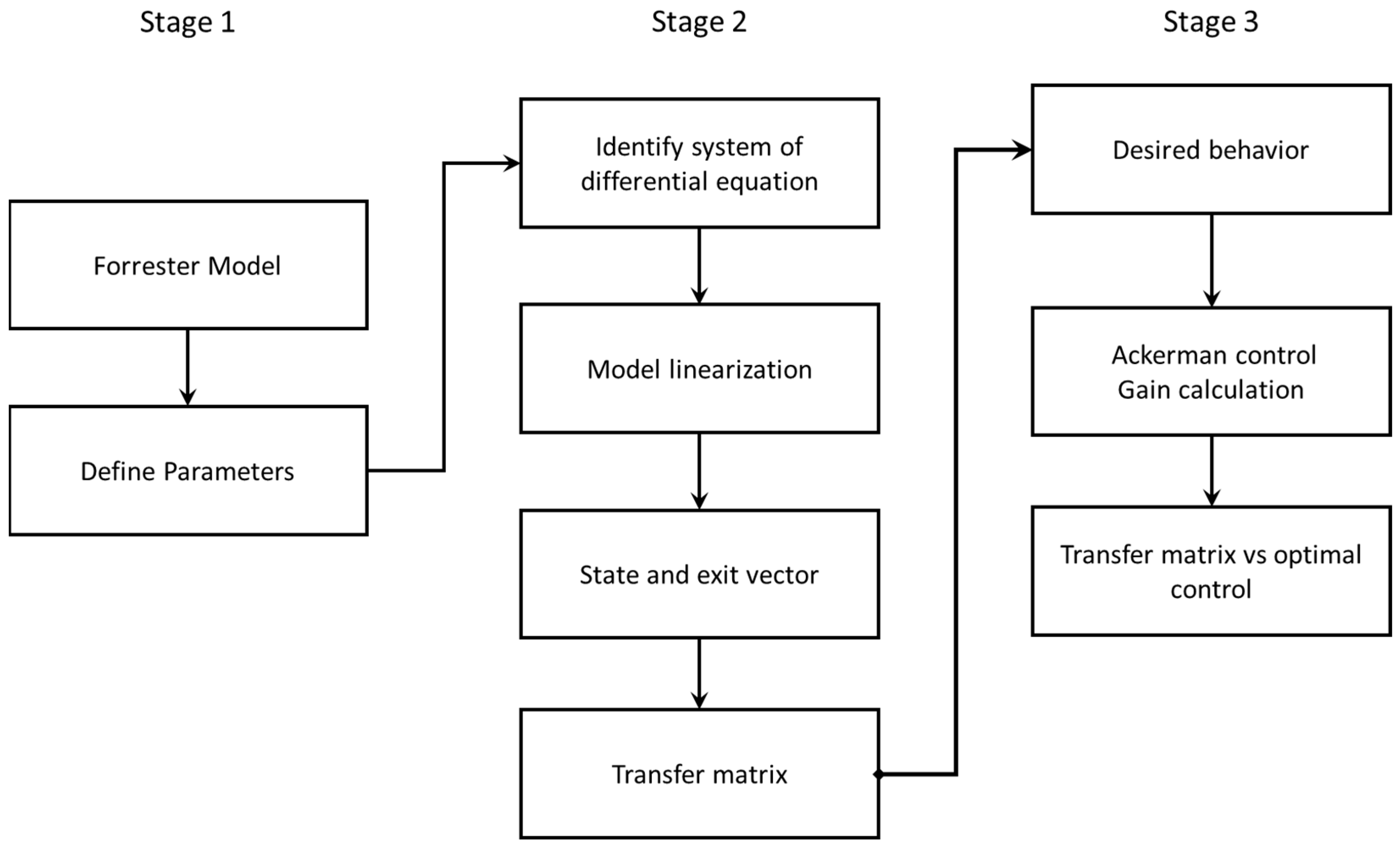
The proposed methodology consists of three fundamental stages for the design and implementation of the control system. In the first stage, the Forrester model is defined, which describes the dynamic behavior of the textile process and allows obtaining a mathematical representation of it. In the second stage, the differential equation of the model is identified and its transformation to state space is carried out, which allows obtaining a matrix representation of the system. In the third stage, the design and implementation of the control system is carried out, using the pole allocation technique through the Ackermann formula, to achieve optimal process performance. It should be mentioned that, in this methodology, three balancing loops, nine auxiliary variables and three flow variables are used, which are defined in the Forrester model and used in the transformation to the state space. The methodology can be seen in Figure 1.

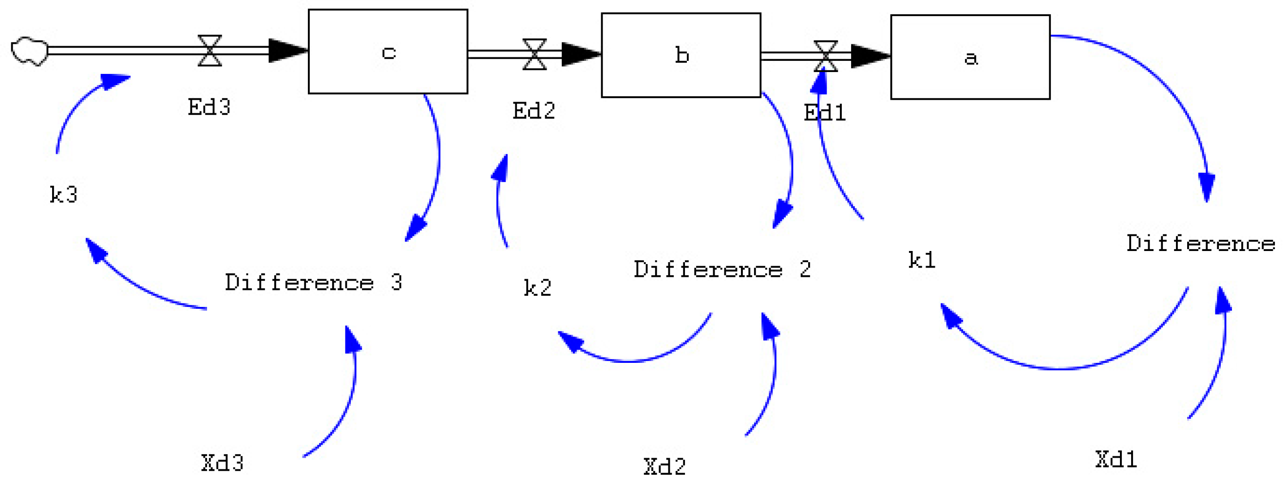
In the first stage, the Forrester diagram is designed, which symbolically represents the level, flow and auxiliary variables of the system. Forrester diagrams are specific system-dynamics (SD) modeling tools, which is a methodology for the study and analysis of complex continuous systems by seeking relationships between subsystems (especially feedback loops). It looks at the system as a “whole”, usually using the computer for simulation. Vensim PLE Plus simulation software is used for this research.

Simulation models created with Vensim are able to reproduce very diverse environments, from physical systems to systems related to a company, or to social and environmental fields. As they are the basis for analyzing the behavior in different time periods of policies to be implemented, in the software the parameters of each state variable are defined, flow or auxiliary, where the state variables correspond to the 3 operations of the textile process under study.

In the second stage, to define a system of differential equations from an SD simulation model represented by the Forrester diagram, one must first identify the variables involved in the system and how they relate to each other to form a whole. Then, the linearization of the state variables must be performed. To linearize the system, all the system variables can be expressed as a linear combination of the state variables. By relating state variables and their derivatives, they are replaced in the system of differential equations.

Subsequently, the state-space representation is performed, which is a mathematical description of the dynamic behavior of a system in terms of state variables, inputs and output. The state equation describes how state variables change over time in response to inputs and the current state of the system. The output equation describes how system outputs relate to state variables and inputs.

Finally, the transfer matrix represents the relationship between system inputs and outputs in terms of state variables and it can be used to analyze the dynamic behavior of the system.

In the third stage, for the design of a controller based on state-space theory, it is necessary to specify the desired behavior of the system. To achieve this desired behavior, the desired poles of the system are calculated. Poles are the eigenvalues of the coefficient matrix A, which define the stability and dynamics of the system. From the natural frequency and the desired damping ratio, the first two poles are calculated. However, as the system has three state variables, a third pole is required. To get the desired third pole, take a zero from the open-loop transfer matrix and cancel with the desired third pole.

Once the desired poles are obtained, a controller can be designed based on state-space theory. After obtaining the desired system poles, the Ackermann technique is used to obtain the k-state feedback matrix. This technique is useful for assigning arbitrary poles to a control system in state space and ensuring system stability. Calculating the k-state feedback matrix is important to control the system properly and achieve the desired behavior.

The methodology will compare the response of the controlled system using the Ackermann technique with the response of the controlled system with the transfer matrix obtained previously. The ability of both controllers to reach the desired poles, the response time, will be evaluated.

This methodology presents a rigorous and systematic approach to designing simulation models in dynamic systems and can be applied in a variety of fields, such as control engineering and economics, among others. The methodology relies on computational tools such as Vensim software to facilitate its implementation.

3. Results

The results based on the methodology developed in this research are presented below.

3.1. Stage 1

3.1.1. Forrester Model

Figure 2 shows a Forrester diagram representing the three processes in the textile sector. The diagram is divided into three horizontal blocks, each of which represents a different process: “Knitting = a“, “Basting = b” and “Ironing = c”. At the top of each block is a box indicating the process name.

3.1.2. Define Forrester Model Parameters

The parameters of the Forrester model for each of the three textile operations are established in

Table 1. Auxiliary variable data and state variable notation.

State Variable	K-Auxiliary	Notation of the Variable
Knitting	0.008541	a
Basting	0.037147	b
Ironing	0.02786	c

, which is presented below.

3.2. Stage 2

3.2.1. Differential-Equations System

To define a system of differential equations from a simulation model, it is necessary to identify the variables involved in the system and how they relate to each other. The variables are listed in Table 1 where the state variables and auxiliary variables are listed. From these variables, the following system of differential equations can be defined; see Equations (7)–(9).

$$\frac{da}{dt}=k1\left(Xd1-a\right)$$

(7)

$$\frac{db}{dt}=k2\left(Xd2-b\right)-k1\left(Xd1-a\right)$$

(8)

$$\frac{dc}{dt}=k3\left(Xd3-c\right)-k2\left(Xd2-b\right)$$

(9)

$da/dt$ represents the rate of change in the number of garments in the knitting process with respect to time.

$db/dt$ represents the rate of change in the number of garments in the basting process with respect to time.

$dc/dt$ represents the rate of change in the number of garments in the ironing process with respect to time.

3.2.2. Linearized State-Space Model

Linearization in state variables is a technique used to approximate the solution of a nonlinear system by linearizing the model around a stable operating point. To linearize the system, it is assumed that all system variables can be expressed as a linear combination of state variables and their derivatives. Nonlinear variables are then replaced by their linear approximation around the stable operating point; see Equations (10)–(15).

$$x_1=a$$

(10)

$${\dot{x}}_1\left(t\right)=\frac{da}{dt}$$

(11)

$$x_2\left(t\right)=b$$

(12)

$${\dot{x}}_2\left(t\right)=\frac{db}{dt}$$

(13)

$$x_3\left(t\right)=c$$

(14)

$${\dot{x}}_3\left(t\right)=\frac{dc}{dt}$$

(15)

Linearization in state variables allows the non-linear system to be described as a linear system with constant coefficients, which facilitates the analysis and solution of the system using linear-algebra techniques. In addition, this technique is useful for the design of linear controllers for the nonlinear system.

The next step after linearization in state variables is to replace these variables in differential equations. This allows us to obtain a set of linear differential equations in the state variables, which can be solved to obtain the temporal evolution of the state variables. The advantage of having linear differential equations is that their solution is simpler and more efficient than those of nonlinear differential equations.

Once you have the linear differential equations in the state variables, you can use control and optimization techniques to design control strategies and improve system performance; see Equations (16)–(18).

$${\dot{x}}_1\left(t\right)=k1\left(Xd1-x_1\right)$$

(16)

$${\dot{x}}_2\left(t\right)=k2\left(Xd2-x_2\right)-k1\left(Xd1-x_1\right)$$

(17)

$${\dot{x}}_3\left(t\right)=k3\left(Xd3-x_3\right)-k2\left(Xd2-x_2\right)$$

(18)

The linearized model is obtained with the state variables defined to carry out the next procedure.

3.2.3. State Equation and Output Vector

We have the input and output equations of the representation in state variables in the following equations; see Equations (2) and (3). To obtain matrix $A$ in its representation in state variables, we must obtain the partial derivatives in each of the equations with respect to the variable of the differential equation. Then, these partial derivatives are organized into a matrix as follows; see Equation (19).

$$\left(\begin{array}{ccc}\frac{\partial {\dot{x}}_1}{\partial x_1}& \frac{\partial {\dot{x}}_2}{\partial x_2}& \frac{\partial {\dot{x}}_3}{\partial x_3}\end{array}\right)$$

$$A=\left(\begin{array}{ccc}-k1& 0& 0\\ k1& -k2& 0\\ 0& k2& -k3\end{array}\right)$$

(19)

This matrix is known as the Jacobian matrix and is the matrix $A$ of the representation in state variables.

Matrix B in the representation in state variables is calculated as follows. The system input variable is identified (in this case, it is the u(t) variable). The partial derivatives of each of the state equations are taken with respect to the input variable. These partial derivatives are placed in a column of matrix B. This column is multiplied by the common system input factor. In this investigation, the input variable of the system is u(t) = 72; see Equation (20).

$$B=\left(\begin{array}{c}k1\\ k2-k1\\ k3-k2\end{array}\right)$$

(20)

Equation (20) indicates that output C is equal to the third state variable, so it can be represented as: where [x1, x2, x3] is the state variable vector. Then, the output derivative can be obtained with respect to time, which is equal to the derivative of the third state variable (x3).

Therefore, the output equation in the representation in state variables is as follows; see Equation (21).

$$C=\left(\begin{array}{ccc}0& 0& 1\end{array}\right)$$

(21)

Variable D represents the direct-transmission matrix (also known as the direct-gain matrix) in the space-state representation of a system. This matrix is used to represent the direct relationship between the input and output of the system, bypassing system dynamics. In some cases, as in the system represented in the SD, the matrix D becomes unnecessary since the output of the system only depends on the state variable and not on the input. In such cases, matrix D is set to zero. This simplifies the representation of the system and reduces the number of calculations needed for analysis and control.

After calculating matrices, A, B, C and D = 0, the representation in system-state variables can be written as follows; see Equations (22) and (23).

$$ẋ=\left(\begin{array}{ccc}-0.008541& 0& 0\\ 0.008541& -0.037147& 0\\ 0& 0.037147& -0.02786\end{array}\right)\left(\begin{array}{c}x1\\ x2\\ x3\end{array}\right)+\left(\begin{array}{c}0.008541\\ 0.028606\\ -0.009287\end{array}\right)\left(\begin{array}{c}u1\\ u2\\ u3\end{array}\right)$$

(22)

$$y=\left(001\right)\left(\begin{array}{c}y1\\ y2\\ y3\end{array}\right)+0$$

(23)

where:

• x is the state vector (x1, x2, x3);
• ẋ is the time derivative of the state vector;
• u is the input vector of the system (u1) and is the output vector of the system (y1);
• A is the state matrix ($3\times 3$);
• B is the input matrix ($3\times 1$);
• C is the output matrix ($1\times 3$);
• D is the direct transmission matrix, which in this case is zero.

3.2.4. Transfer Matrix

Therefore, to simulate the behavior of the system, the differential equation describing the time evolution of the state vector x and the equation relating the output vector y to the state vector x can be used. The transfer matrix G(s) is calculated as the ratio between the output Laplace transform (x3) and the input Laplace transform (u), with the initial conditions equal to zero; see Equation (4).

Where C is the output matrix, which in this case is [0 0 1];

A is the matrix of system coefficients, previously calculated;

B is the input matrix, which in this case is [0; 0; 1].

sI is the identity matrix multiplied by s, which is used to do the subtraction operation $sI-A.$ The result of this operation is a transfer function G(s) in terms of the complex variable s, which represents the relationship between the input and output of the system in the frequency domain. We proceed to solve the matrix operation that is inside the parentheses; see Equation (24).

$$\left(sI-A\right)=s.\left(\begin{array}{ccc}1& 0& 0\\ 0& 1& 0\\ 0& 0& 1\end{array}\right)-\left(\begin{array}{ccc}-0.008541& 0& 0\\ 0.008541& -0.037147& 0\\ 0& 0.0037147& -0.02786\end{array}\right)$$

(24)

The following matrix is obtained; see Equation (25).

$$\left(sI-A\right)=\left(\begin{array}{ccc}s+0.00851& 0& 0\\ -0.008541& s+0.037147& 0\\ 0& -0.037147& s+0.02786\end{array}\right)$$

(25)

To obtain the transfer matrix, the equation must be inverted as follows; see Equation (26).

$${(sI-A)}^{-1}=\frac{adj\left(sI-A\right)}{det\left(sI-A\right)}$$

(26)

The matrices obtained from the system are replaced in the transfer matrix G(s), the respective operations are carried out and the output transfer matrix is calculated; see Equation (27).

$$G\left(s\right)=\frac{-0.009827s^2+0.0006386s+8.834\ast {10}^{-6}}{s^3+0.07354s^2+0.00159s+8.834\ast {10}^{-6}}$$

(27)

3.3. Stage 3

3.3.1. Define Desired Behavior

The zeta $(\sigma$) parameter, also known as the damping coefficient, is a value used in dynamic system analysis to describe a system’s damped response. It indicates the amount of damping present in the system and affects its behavior in terms of stability, response time and damping. The zeta value varies between 0 and 1, where 0 represents a sub-damped system, 1 indicates a critically damped system and values above 1 represent over-damped systems. Another important parameter in the analysis of dynamic systems is natural frequency. The natural frequency, represented by the letter omega ($w_n$), is a measure of the speed at which a system will vibrate or oscillate in the absence of damping or external forces. For the calculation of the establishment time ($t_{sa}$), a commonly used criterion is to consider that the response has reached the stable state when it is within 2% of the final value. In this case, the set time can be approximated using the following Formula (29).

In the pole assignment, a desired behavior of the controlled system is sought, so poles are chosen that generate the type of response expected from the system. In this case, it is sought to obtain a slightly damped behavior, so poles with a value greater than 1 are chosen. In addition, the system is intended to have an establishment time of approximately 320 min and a settlement time of about 125 min for the third operation. To calculate the natural frequency of the system, Equations (28) and (29) are used to obtain the desired pole values.

$$\sigma =1.1$$

(28)

$$w_n=4/(\sigma \ast t_{sa})=0.0291$$

(29)

Equation (30) shows the desired poles of the system, which are obtained from the desired natural frequency ($w_n$) and damping ratio ($\sigma$). The poles are represented as complex conjugate values, since the system is second-order, plus a cancellation of poles and zeros is performed to use the second-order system. In this case, low damping behavior is desired, so the damping ratio is set to 0.1 and the natural frequency is calculated from the desired settlement time and establishment time values.

$$s_{\mathrm{1,2}}=-w_n\ast \sigma +/-w_n\left(\sqrt{{\sigma }^2-1}\right)$$

(30)

Replacing the values results in the two desired poles being the following; see Equation (31).

$$s_1=-0.0187,s_2=-0.0453,$$

(31)

In the case of Equation (32), a specific pole $\left(s_3\right)$ is being manually assigned to achieve a desired behavior in the system. To get that desired pole, you take a zero from the open-loop transfer matrix and cancel it with the desired pole. This technique is called pole-zero cancellation. Pole-zero cancellation involves adding a zero in the controller transfer function to cancel an unwanted pole in the system transfer function. In this case, a pole in the open-loop transfer matrix is canceled with a zero in the controller transfer function, resulting in the desired pole in the closed-system transfer function.

$$s_3=-0.0128$$

(32)

With the desired poles defined, you can perform pole assignment to obtain the driver gain that ensures the desired system behavior.

3.3.2. Control Ackermann—Calculation of Gains

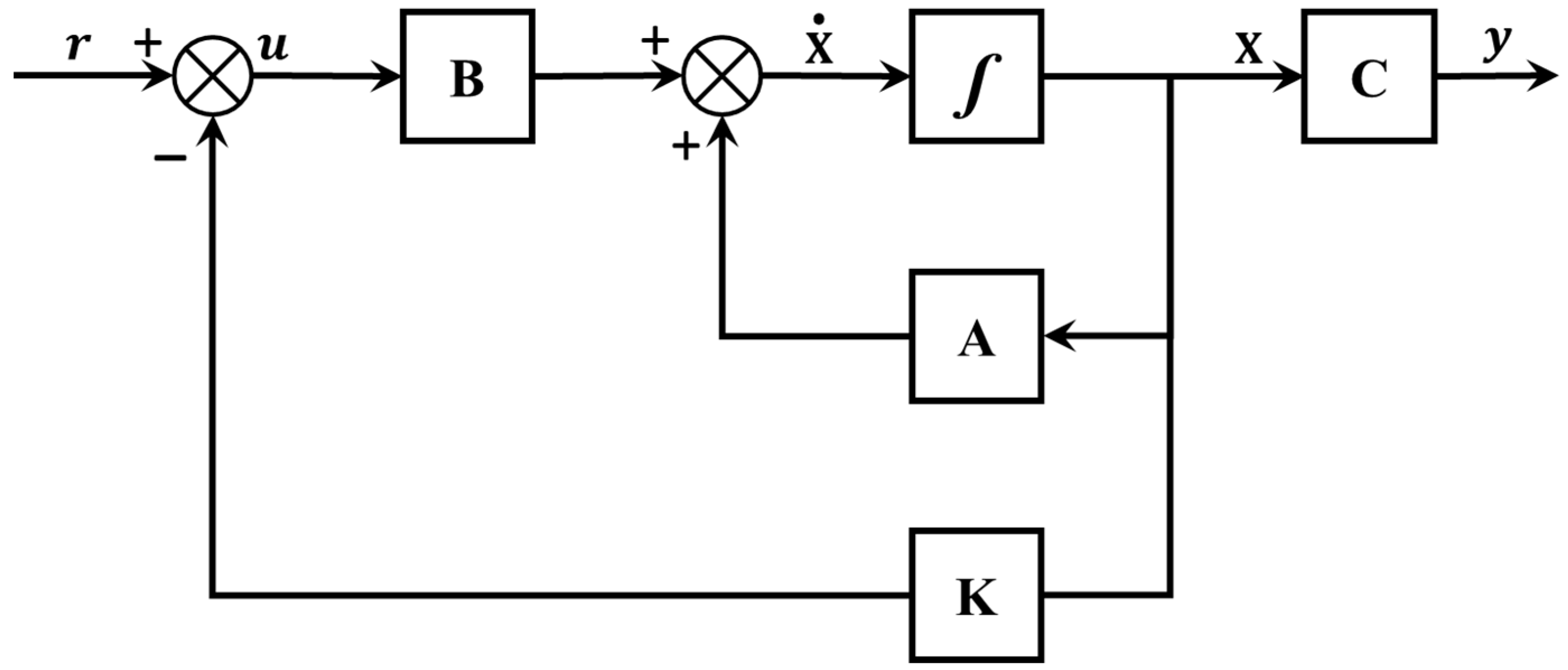
When we are faced with a control problem in state variables, one of the ways to find the gain matrix k of the state feedback is by using Ackermann formula. This formula allows direct calculation of the feedback-gain matrix in the state space, starting from the following equation if the system is in the controllable form; see Figure 3.

For the calculation of Ackermann gains, the following equation is used; see Equation (33).

$$k=\left(00\dots \dots \dots 1\right){\left(C\right)}^{-1}\varnothing \left(A\right)$$

(33)

where matrix C is the controllability matrix of the system and ∅(A) can be expressed as the following equation; see Equation (34).

$$\varnothing \left(A\right)={\lambda }^n+{\alpha }_1{\lambda }^{n-1}+{\alpha }_2{\lambda }^{n-2}+\dots +{\alpha }_{n-1}\lambda +{\alpha }_n$$

(34)

In this equation, ${\alpha }_{1,}{\alpha }_{2,\dots ,}{\alpha }_n$ are the coefficients of the desired characteristic equation.

Where the desired poles of the system are already available for the research carried out, the desired characteristic equation is calculated from these; see Equation (35).

$$\left(s+0.0187\right)\left(s+0.0453\right)\left(s+0.0128\right)$$

(35)

By multiplying the three poles, the desired equation, Equation (36),

$$∆\left(\lambda \right)=s^3+0.07681s^2+0.00166s+1.084\ast {10}^{-5}$$

(36)

is obtained.

$$\begin{array}{ll}\varnothing \left(A\right)& ={\left(\begin{array}{ccc}-0.008541& 0& 0\\ 0.008541& -0.037147& 0\\ 0& 0.037147& -0.02786\end{array}\right)}^3\\ & +0.07681{\left(\begin{array}{ccc}-0.008541& 0& 0\\ 0.008541& -0.037147& 0\\ 0& 0.037147& -0.02786\end{array}\right)}^2\\ & +0.00166\left(\begin{array}{ccc}-0.008541& 0& 0\\ 0.008541& -0.037147& 0\\ 0& 0.037147& -0.02786\end{array}\right)+1.084\\ & \ast {10}^{-5}\left(\begin{array}{ccc}-0.008541& 0& 0\\ 0.008541& -0.037147& 0\\ 0& 0.037147& -0.02786\end{array}\right)\end{array}$$

(37)

By performing the matrix operations and adding each of the operations, Equation (38) is obtained.

$$\varnothing \left(A\right)={10}^{-5}\left(\begin{array}{ccc}0.1592& 0& 0\\ -0.0623& 0.3681& 0\\ 0.1035& -0.5055& 0.2417\end{array}\right)$$

(38)

We proceed to obtain the controllability matrix of the system; see Equation (39).

$$C=\left(bAb{A}^{2}b\right)$$

(39)

where, by replacing and performing the operations in each of the positions of the matrix, the result is as follows; see Equation (40).

$$\begin{gathered} C=\left(\begin{array}{ccc}0.008541& -0.0001& 0.0062\ast {10}^{-4}\\ 0.028606& -0.0010& 0.3614\ast {10}^{-4}\\ -0.009287& 0.0013& -0.0001\end{array}\right) \\ K=\left[001\right]{\left(\begin{array}{ccc}0.008541& -0.0001& 0.0062\ast {10}^{-4}\\ 0.028606& -0.0010& 0.3614\ast {10}^{-4}\\ -0.009287& 0.0013& -0.0001\end{array}\right)}^{-1} \\ \ast {10}^{-5}\left(\begin{array}{ccc}0.0921& 0& 0\\ -0.0067& 0.1147& 0\\ 0.0104& -0.0528& 0.1015\end{array}\right) \end{gathered}$$

(40)

The following vector of Ackermann k, of 1 × 3, is obtained by having three columns and one row; see Equation (41).

$$k=\left(\begin{array}{ccc}0.4431& -0.0666& -0.1495\end{array}\right)$$

(41)

To get the new Ak, it is substituted into the feedback equation; see Equation (42).

$$\left(\begin{array}{ccc}-0.0123& 0.0006& 0.0013\\ -0.0041& -0.0352& 0.0043\\ 0.0041& 0.0365& -0.0292\end{array}\right)$$

(42)

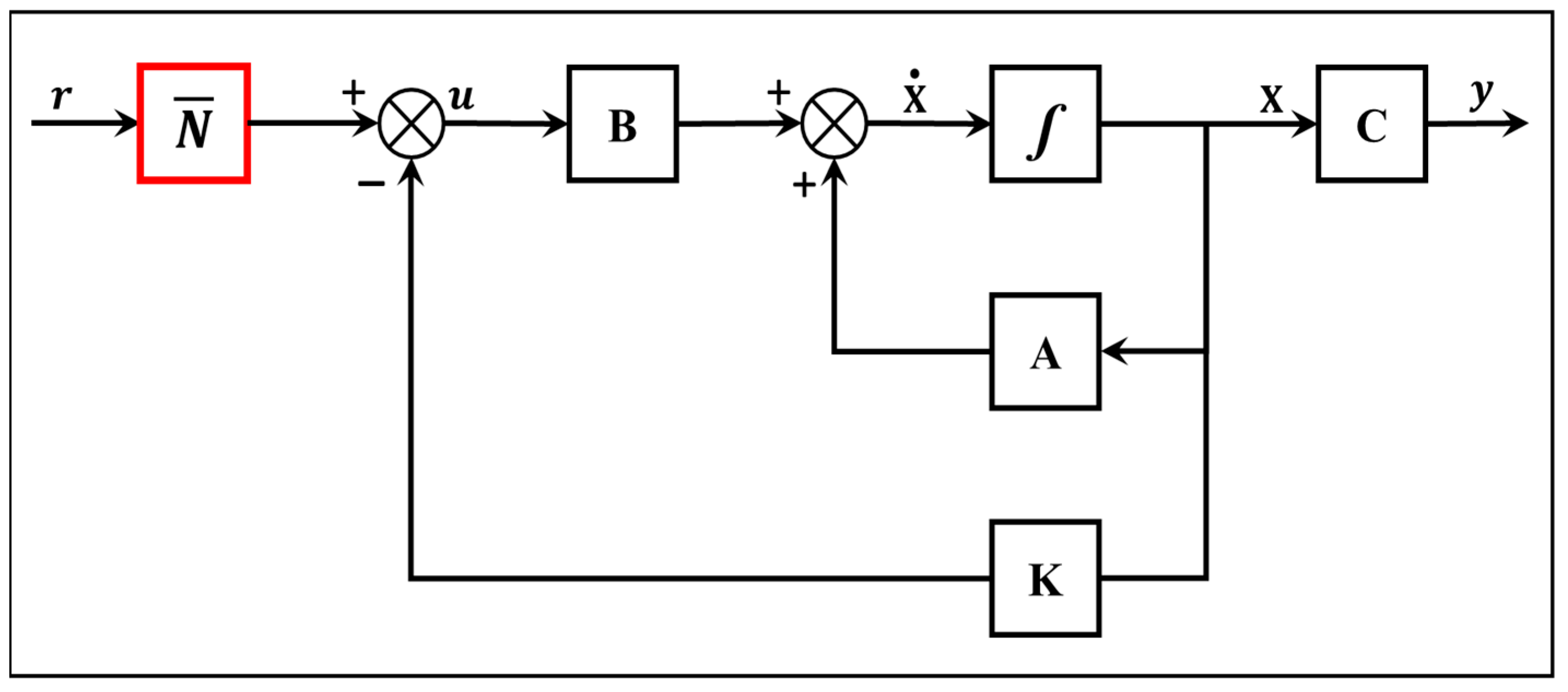
To obtain a model with different inputs and that follows a reference, block N is added at the input of the pole protection block diagram; a control is carried out by following a reference, for this case a gain of precompensation, whose deduction is as follows; see Figure 4.

The formula that represents the value of the precompensation gain is given under the following equation; see Equation (43).

$$N=\frac{1}{C{(A-Bk)}^{-1}B}$$

(43)

Plugging the data into the above equation, we get a gain of N = 1.2269 for the precompensation gain. The transfer function for the new pole assignment including the regulation gain for a reference remains as follows; see Equation (44).

$$G_2\left(s\right)=\frac{-0.01139s^2+0.0007834s+1.084\ast {10}^{-5}}{s^3+0.07681s^2+0.001666s+1.084\ast {10}^{-5}}$$

(44)

where, by equaling the denominator to zero, the eigenvalues and the desired roots are obtained, in order to obtain control by assigning poles and obtain a faster behavior of the operation.

3.3.3. Graph Transfer Matrix vs. Optimum Control

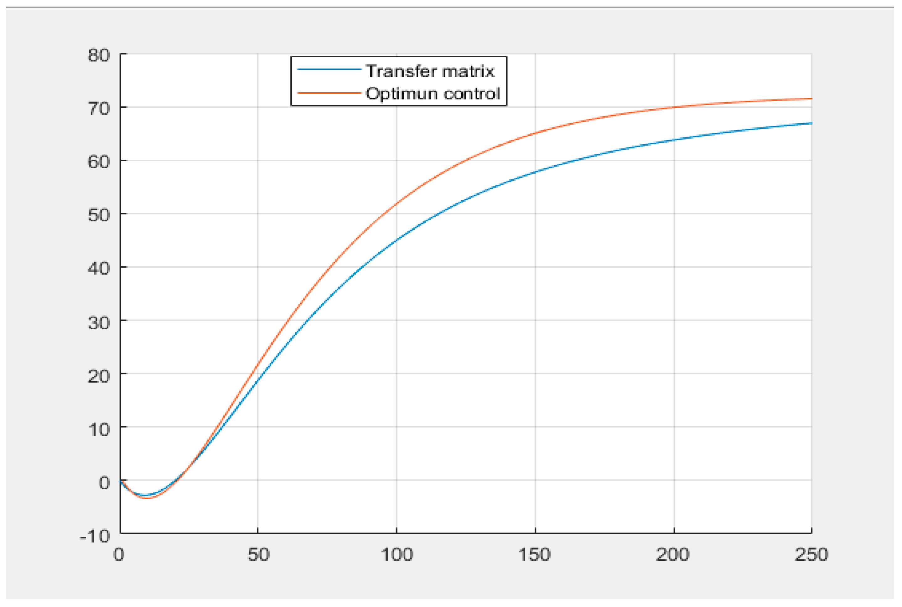
The responses to a step input with an amplitude of 72, of the transference matrix and with optimal control, can be seen below. By equaling the denominator to zero, the eigenvalues and the desired roots are obtained, in order to obtain control by assigning poles and obtain a faster behavior of the operation. In Figure 5, the x axis corresponds to the time in minutes, while the y axis represents the number of textile pieces obtained as a target. This means that the graph shows how the number of parts produced varies over time.

Figure 5 shows a comparison between the transfer-matrix response and the optimal Ackermann control for a staggered input with an amplitude of 72. The transfer-matrix response is represented by the curve in blue, while the optimal Ackermann control response is represented by the curve in red. The graph shows that the optimal Ackermann control response is faster and has fewer oscillations than the transfer-matrix response. This is because the optimal Ackermann control uses complete system information to calculate the control action, while the transfer matrix only takes into account input and output information.

In addition, it can be noticed that during the period of 0 to 20 min, the optimal control response presents a slight negative oscillation due to the state variable b being filled before the input c reaches its maximum value. However, after this period, the response is stabilized and the control of the output state variable of the simulation proposed in SD is achieved. In summary, the figure shows how optimal Ackermann control can improve the system response compared to the transfer matrix, allowing better control of the output state variable and greater efficiency in the proposed simulation process.

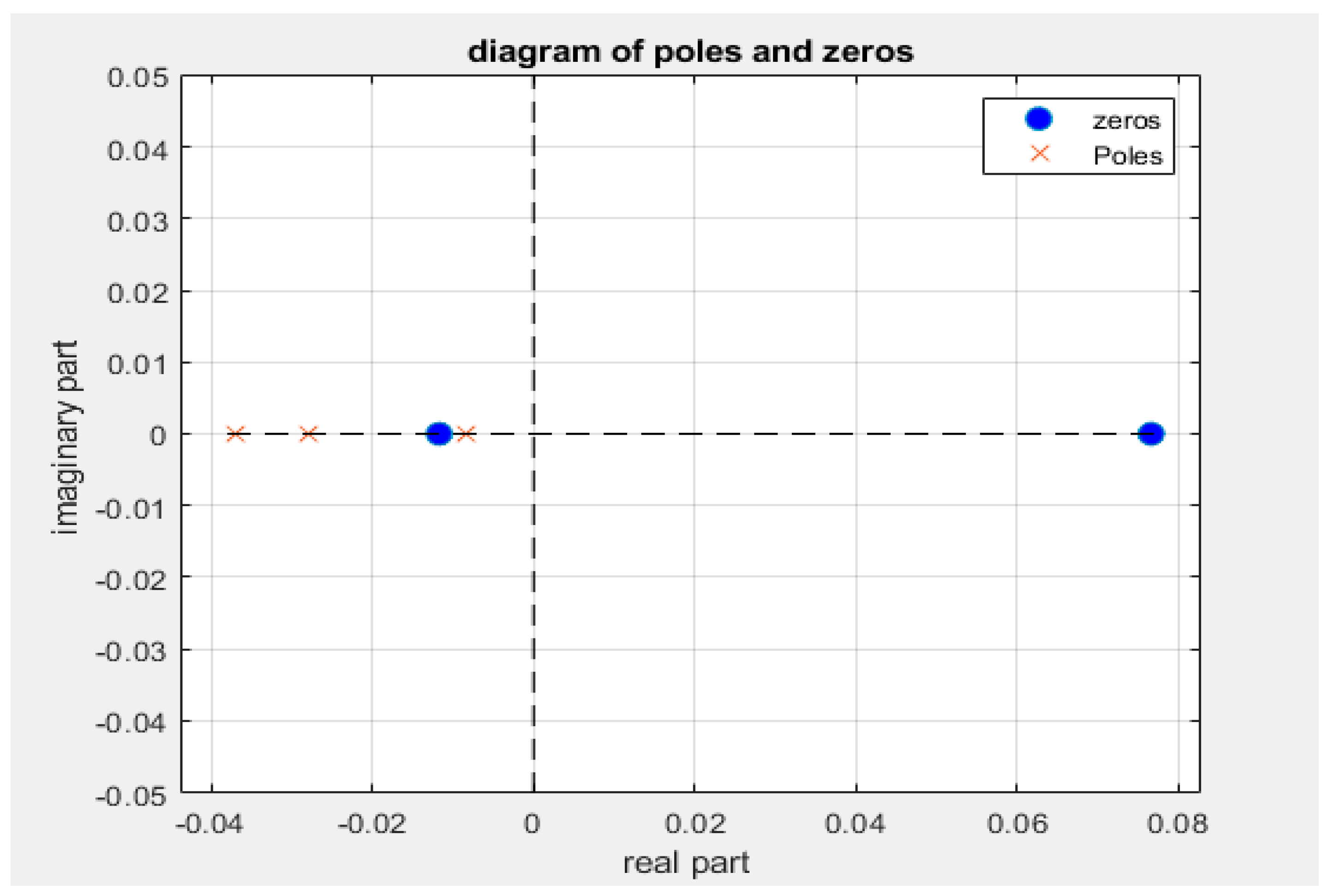
Pole and Zero Diagram Transfer Function vs. Optimal Control

The pole and zero diagram of a transfer function is a useful tool for analyzing and understanding the behavior of a control system. It allows visualization of the location of the poles and zeros in the complex plane, which provides important information about the stability and response of the system. Figure 6 shows the diagram of poles and zeros in the imaginary and the real plane of the transfer function. The following poles and zeros were identified. See Equations (45) and (46).

$$\mathrm{P}\mathrm{o}\mathrm{l}\mathrm{e}\mathrm{s}:-0.0371,-0.0279\mathrm{a}\mathrm{n}\mathrm{d}-0.0085$$

(45)

$$\mathrm{Z}\mathrm{e}\mathrm{r}\mathrm{o}\mathrm{s}:0.0767\mathrm{a}\mathrm{n}\mathrm{d}-0.0117$$

(46)

All poles have the imaginary part equal to zero and are located on the left side of the complex plane. Since the poles have the imaginary zero part and are on the left side of the complex plane, it can be concluded that they are stable. Figure 6 shows a positive zero, which does not directly affect the stability of the system, since its location does not determine the stability or instability of the system. However, zeros can affect the frequency response and form of the system response.

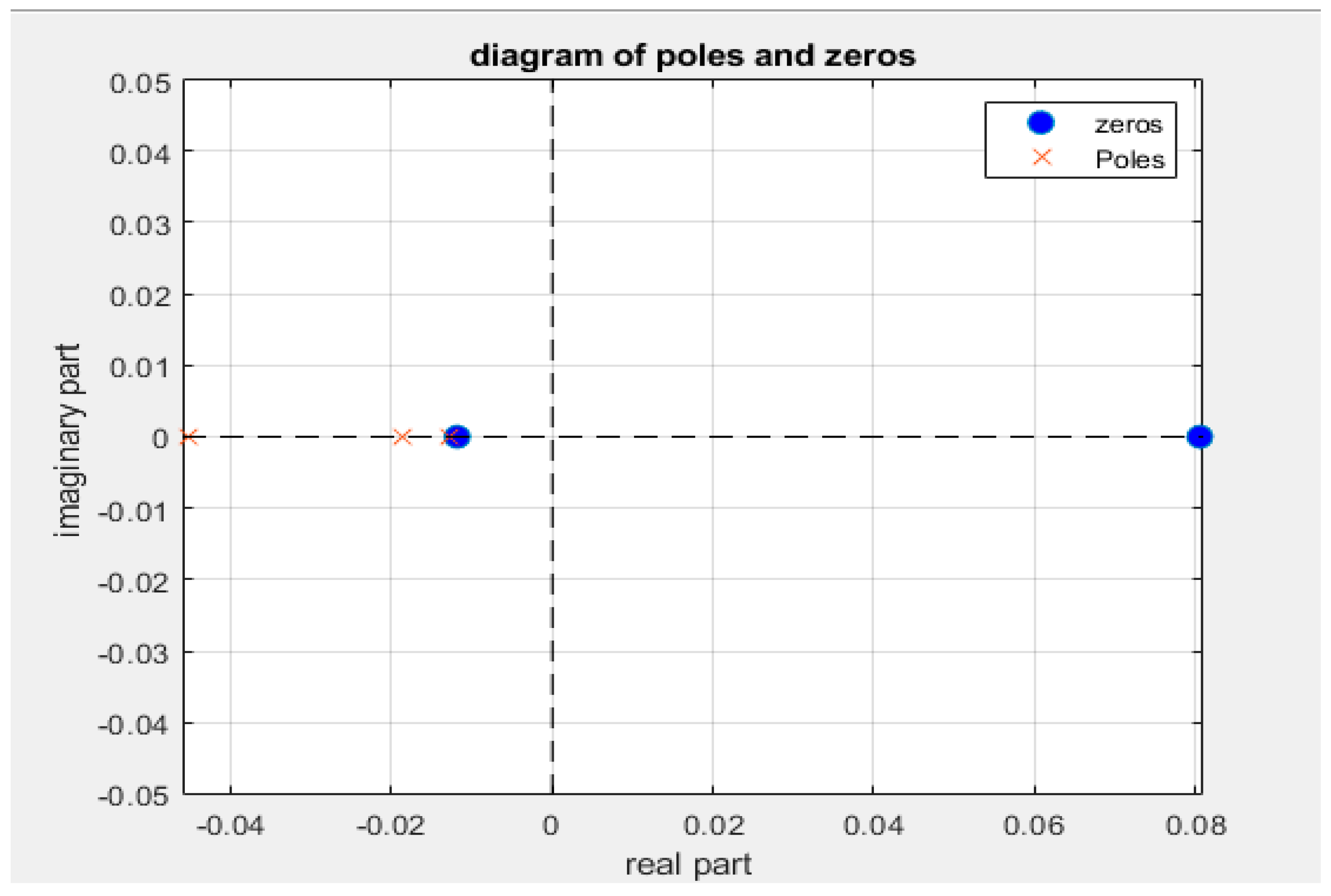
Comparing the poles and zeros before and after applying the Ackermann control, we can see how they moved and the impact on the system response.

Before the Ackermann control, the poles and zeros were as follows:

$$\mathrm{P}\mathrm{o}\mathrm{l}\mathrm{e}\mathrm{s}:-0.0371,-0.0279,-0.0085.$$

$$\mathrm{Z}\mathrm{e}\mathrm{r}\mathrm{o}\mathrm{s}:0.0767,-0.0117.$$

After applying the Ackermann control, the poles and zeros changed to: see Equations (47) and (48).

$$\mathrm{P}\mathrm{o}\mathrm{l}\mathrm{e}\mathrm{s}:-0.0453,-0.0187,-0.0128$$

(47)

$$\mathrm{Z}\mathrm{e}\mathrm{r}\mathrm{o}\mathrm{s}:0.0806,-0.0118$$

(48)

We note in Figure 7 that the poles moved to different locations in the complex plane. The absolute values of the poles increased slightly, indicating that the system became a little faster in its response. This may involve greater baseline tracking and faster response to changes in system conditions.

Zeros also moved, although the changes were not as significant. These changes can have subtle effects on the frequency response and the form of the system response. The type of behavior without oscillations did not vary. This indicates that the Ackerman control maintained the stability of the system and prevented unwanted oscillations.

The system exhibited an overdamped response, which means that it converged rapidly towards its stable state without excessive oscillations. This feature is desirable in many applications where a fast and stable system response is required. In summary, selecting a damping value greater than 1 ensures an over-damped behavior in the system, where the poles remain real and there is no presence of oscillations in the transient response. This provides stability and rapid system response.

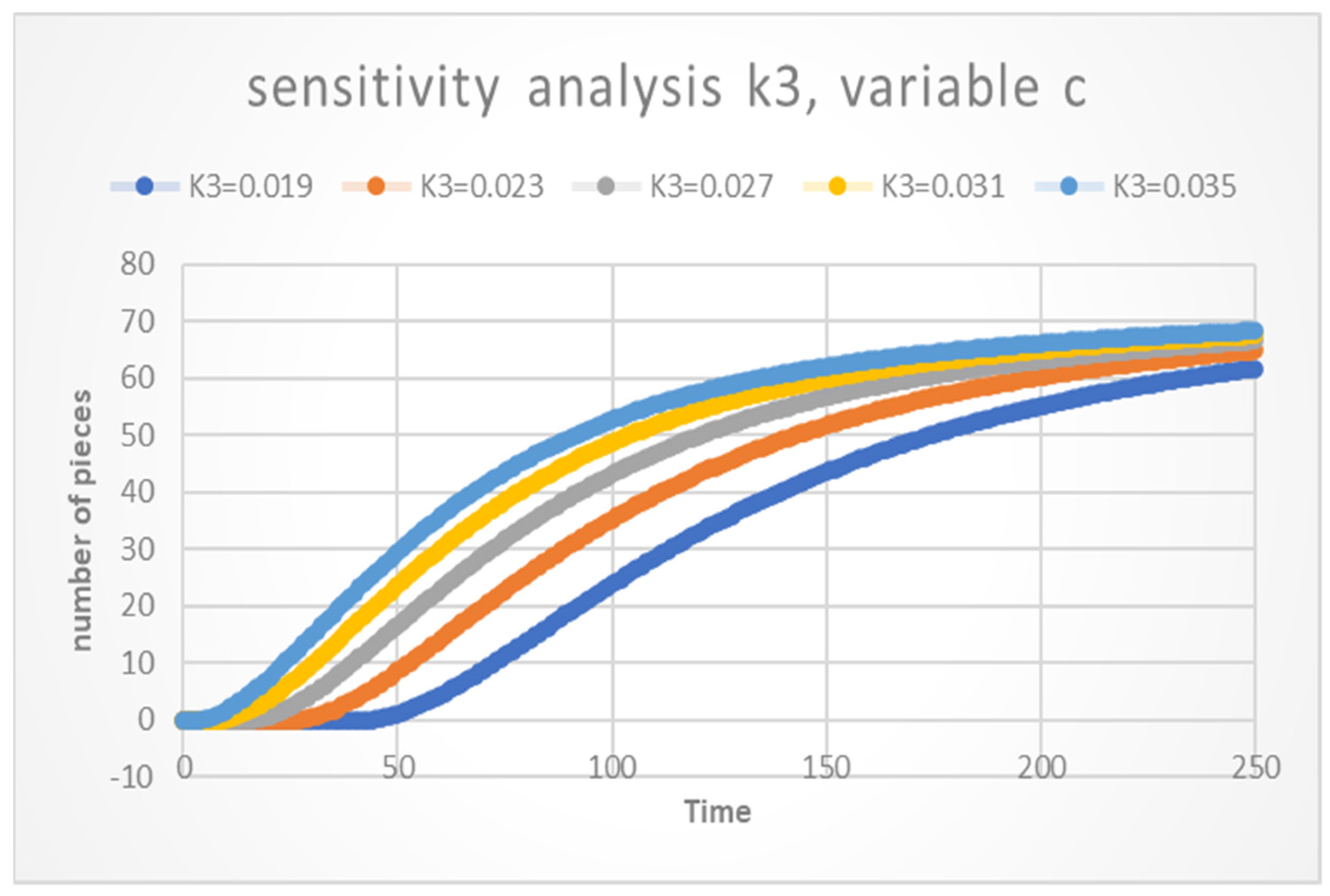
Sensitivity Analysis of Simulation Models

Figure 8 shows a sensitivity analysis for different scenarios of variable c. The value of k3 varies from 0.019 to 0.035, and in intervals of 0.004, where it provides us with important information when seeing different scenarios that change the values of k3, but none identifies the set time of 125 min which seeks 63.2% of the final value and a settlement time of approximately 180 min of (95–98%) of the final value.

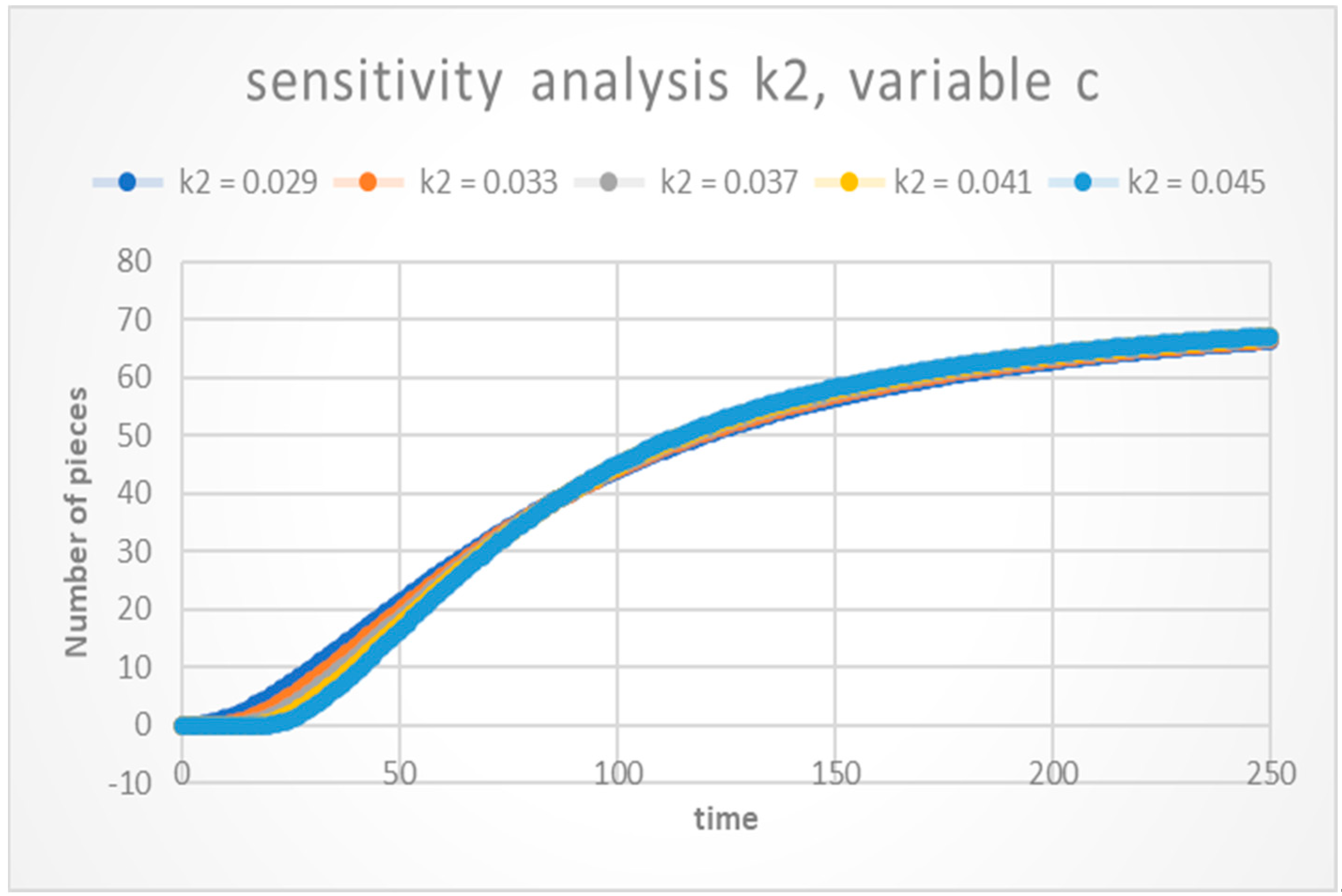
Figure 9 shows a sensitivity analysis for different scenarios of variable c. The value of k1 varies from 0.029 to 0.045, and in intervals of 0.004. It is useful to have different results in the simulation model, which provides multiple results, but none identifies the set time above 125 min looking for 63.2% of the final value and a settlement time of approximately 180 min of (95–98) % of the final value, which is the maximum achieved.

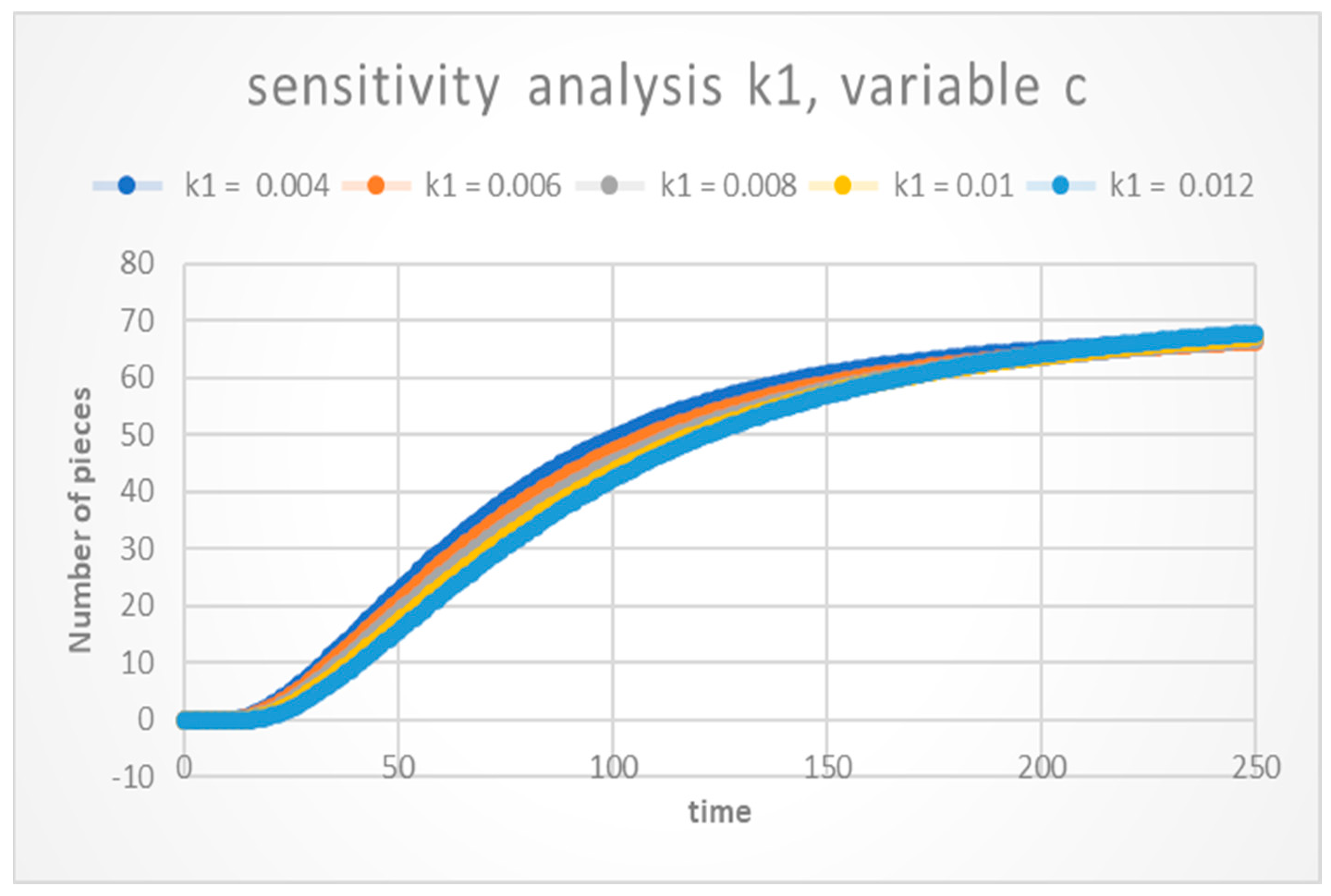
Figure 10 shows a sensitivity analysis for different scenarios of variable c. The value of k1 varies from 0.004 to 0.0012, and in intervals of 0.002. It is useful to have different results in the simulation model, which provides multiple results, but none identifies the set time above 125 min looking for 63.2% of the final value and a settlement time of approximately 180 min of 98% of the final value, which is the maximum achieved.

In conclusion, sensitivity analysis is a valuable tool for evaluating the impact of variables on model results and exploring different scenarios in the context of the present research. However, it is essential to take into account the limitations inherent in this technique and consider other relevant factors to make informed decisions. In this study, a methodology based on the state space and control approach has been implemented using the Ackermann technique. This methodology allows the obtaining of the optimal values required when considering the internal and external dynamics of the system, and when relating the output equation with the input using the transfer function. It is important to note that the sensitivity analysis, although valuable, should be complemented by other techniques and approaches to obtain a more complete and accurate understanding of the system under study.

4. Conclusions

The present investigation proposes an analytical methodology for the models of SD applied in the textile sector, which can be replicated in multiple sectors where there is application of SD. The analysis is by means of the state-space-matrix technique of the Forrester models, through modern control techniques. In previous works, it had been possible to obtain a transfer matrix that describes the plant of the system and the behaviors before different inputs, but the main objective of this research was to achieve, through the manipulation of the control variables, a domain over the output variables, so that they reach preset values (set point).

The manipulation of the control variables was carried out by means of the Ackermann control technique to obtain the profit matrix of our system in order to improve the response time of the output variable of the simulation model of SD. Comparison of the transfer matrix with the optimal control was made, where a response of approximately 125 min was obtained to achieve 98% of the system goal and for the initial mathematical model of approximately 240–250 min. In short, system dynamics and control engineering are interconnected disciplines used to analyze and model complex systems in different areas of engineering and science. In this scientific paper, these disciplines were used to model and analyze a complex system and design control systems to regulate its behavior and maximize system efficiency.

There are several possible lines of research that could be addressed in the future in relation to the study presented in this scientific paper. These include the implementation of optimal control in real systems. It would be interesting to carry out a practical implementation of the optimal control techniques proposed in this study, in real systems in the textile sector or other sectors, in order to assess their effectiveness in practice and to make adjustments where necessary.

A sensitivity analysis was performed in the proposed model to assess how the results would be affected if changes were made to the parameters or conditions of the system. Where it was evidenced that a sensitivity analysis produced useful results in the research, when varying the parameters, but these could not be obtained in a simple way, the time required establishment. The methodology proposed in this study is a more efficient alternative when it comes to the behaviors required in specific, and the methodology could be applied to other complex systems in different sectors, such as food, pharmaceuticals and energy, among others.

Regarding the design of more advanced control systems, this study used the Ackermann control technique, but there are other, more advanced control techniques that could be explored in the future, such as predictive control, blurred control, and adaptive control, among others. It would be interesting to assess how these techniques would compare with the technique used in this study and how effective they would be in different systems.

Ackerman’s control technique is used for designing optimal controllers in dynamic systems, while Forrester’s system-dynamics simulation is a tool for modeling and analyzing the behavior of complex systems over time. By combining these two techniques, it is possible to obtain a comprehensive approach to evaluate and optimize management in different industries.

With the proposed methodology, it is possible to divide any process into n operations and analyze each of them through rolling loops. This involves establishing differential equations for each operation and then establishing the corresponding state equations. When obtaining the transfer matrix, you can use the Ackermann technique to optimize the parameters under study for any sector. This approach allows a detailed and complete analysis of each individual operation in the process, which facilitates the optimization of parameters and the design of effective control strategies. By dividing the process into smaller operations and addressing them individually, you can identify potential bottlenecks or areas for improvement and apply specific adjustments to each.

By using the Ackermann technique, the optimal values for system parameters can be determined, contributing to improved performance and efficiency. This control technique provides a methodology for adjusting and optimizing the parameters of each operation, taking into account the objectives and constraints of the sector under study. In short, by breaking a process into operations and applying balancing loops, each can be individually analyzed and optimized. The use of state equations, a transfer matrix and the Ackermann technique allows for better control and the optimization of parameters in any sector under study.