Article

Hyperspectral Image Classification Based on Fusion of Convolutional Neural Network and Graph Network

1
Changchun Institute of Optics, Fine Mechanics and Physics, Chinese Academy of Sciences, Changchun 130033, China
2
University of Chinese Academy of Sciences, Beijing 100049, China
3
College of Computer Science and Technology, Changchun Normal University, Changchun 130033, China
*
Author to whom correspondence should be addressed.
Appl. Sci. 2023, 13(12), 7143; https://doi.org/10.3390/app13127143
Submission received: 20 April 2023 / Revised: 11 June 2023 / Accepted: 12 June 2023 / Published: 14 June 2023
(This article belongs to the Special Issue Recent Advances in Robotics and Intelligent Robots Applications)

Abstract

:
Convolutional neural networks (CNNs) have attracted significant attention as a commonly used method for hyperspectral image (HSI) classification in recent years; however, CNNs can only be applied to Euclidean data and have difficulties in dealing with relationships due to their limitations of local feature extraction. Each pixel of a hyperspectral image contains a set of spectral bands that are correlated and interact with each other, and the methods used to process Euclidean data cannot effectively obtain these correlations. In contrast, the graph convolutional network (GCN) can be used in non-Euclidean data but usually leads to over-smoothing and ignores local detail features due to the need for superpixel segmentation processing to reduce computational effort. To overcome the above problems, we constructed a fusion network based on the GCN and CNN which contains two branches: a graph convolutional network based on superpixel segmentation and a convolutional network with an added attention mechanism. The graph convolutional branch can extract the structural features and capture the relationships between the nodes, and the convolutional branch can extract detailed features in the local fine region. Owing to the fact that the features extracted from the two branches are different, the classification performance can be improved by fusing the complementary features extracted from the two branches. To validate the proposed algorithm, experiments were conducted on three widely used datasets, namely Indian Pines, Pavia University, and Salinas. An overall accuracy of 98.78% was obtained in the Indian Pines dataset, and overall accuracies of 98.99% and 98.69% were obtained in the other two datasets. The results show that the proposed fusion network can obtain richer features and achieve a high classification accuracy.

1. Introduction

Hyperspectral imaging technology combines imaging technology with spectral technology and has achieved wide application in recent years. With the advancement of hyperspectral imaging technology, hyperspectral imaging systems can simultaneously acquire abundant spectral information and two-dimensional spatial information of a feature and then form a hyperspectral image (HSI) [1,2,3]. Therefore, hyperspectral imaging technology has become a hotspot for research due to its rich spectral and spatial information. An HSI provides from tens to hundreds of continuous spectral bands [4]. The abundance of spectral information greatly enhances the ability to distinguish objects. Therefore, an HSI is commonly used in disaster monitoring, vegetation classification, fine agriculture, and medical diagnosis due to its extremely high spectral resolution [1,2,5].
As the focus of the field of hyperspectral image analysis, the HSI classification task has always received significant attention from scholars. Hyperspectral image classification aims to classify each pixel point in the image [6]. In the early days, most HSI classification methods mainly relied on some traditional machine learning algorithms [7] which were mainly divided into two processes: traditional manual feature engineering and classifier classification [8]. Feature engineering aims to process data based on knowledge so that the processed features can be better used in subsequent classification algorithms. Commonly used feature engineering methods include principal component analysis (PCA), independent component analysis (ICA), and other dimensionality reduction methods.
Typical classification algorithms include the support vector machine (SVM) [9], random forest (RF) [10], and k-nearest neighbor (KNN) [11], etc. [12,13]. The above machine learning approaches only focus on the spectral information of an HSI. It is inaccurate to use the spectral information only for the classification task, thus limiting the improvement in the classification accuracy and the gradual elimination of spectral information.
As a result of the triumph of deep learning in areas such as computer vision, many approaches based on deep learning have also been adopted for hyperspectral image classification [14]. Among the deep learning methods, convolutional neural networks (CNNs) [15] have become a popular method for hyperspectral image classification due to their excellent performance. Deep-learning-based methods represented by CNNs have replaced traditional machine-learning-based HSI classification methods and have become a research hotspot [16].
Deep learning methods of 1D-CNN [17] and 2D-CNN were first applied to hyperspectral image classification, and the performance surpassed machine learning methods. However, the above methods suffer from the underutilization of spatial and spectral information. Therefore, the 3D-CNN model [16] was proposed, which can extract spatial–spectral features simultaneously and therefore obtain better classification results, but the model has a large computational burden. To extract richer features, some scholars have proposed a hybrid spectral CNN (HybridSN) [18] which combines 3D-CNN and 2D-CNN to exploit the spatial–spectral features of an HSI with less computational burden than 3D-CNN.
With the purpose of finding correlations between data, highlighting important features, and ignoring irrelevant noise information, an attention mechanism has been proposed. Li et al. proposed a two-branch double attention network (DBDA) [19] which contained two branches to extract spatial and spectral features and added an attention mechanism to obtain better classification results. In order to capture richer features, deeper network layers are needed, but the deeper network layers will lead to computational complexity and make the model training difficult. Zhong et al. introduced a residual structure based on the 3D-CNN model [20], constructed a spectral residual module and a spatial residual module, and achieved more satisfactory classification results.
Although the classification results achieved by CNN-based classification methods have been good, there are still some limitations. First, the CNN is designed for Euclidean data, and the traditional CNN model can only convolve regular rectangular regions, so it is difficult to obtain complex topological information. Second, CNNs cannot capture and utilize the relationship between different pixels or regions in hyperspectral images; they can only extract detailed features in the local fine region, but the structure features and dependency relationship between the nodes may provide useful information for the classification process [21,22].
In order to obtain the relationship between objects, graph convolutional networks (GCNs) have been developed rapidly in recent years [23]. GCNs are designed to process graph-structured data. CNNs are used for processing Euclidean data such as images, which are a regular matrix. Therefore, no matter where the convolution kernel of a CNN is located in the image, the consistency of the result of the operation is guaranteed (translational invariance). However, the graph-structured data are non-Euclidean data, and the graph structure is irregular, so it is impossible to apply the CNN on graph data. The graph convolution is designed to resolve this situation. The most important innovation of the GCN is to overcome the inapplicability of translation invariance on non-Euclidean data, so it can be applied to extract the features of the graph structure.
Kipf et al. proposed the GCN model [24] which is able to operate on non-Euclidean data and extract the structural relationship between different nodes [21]. Some scholars have attempted to apply the GCN to hyperspectral classification tasks [25], and various studies have shown that the classification results are not only affected by spectral information but are also related to the spatial structure information of the pixels [22,26]. By treating each pixel or superpixel in the HSI as a graph node, the hyperspectral image can be converted into graph-structured data, and then the GCN can be used to obtain the spatial structure information in the image and provide a more effective information for the classification. Hong et al. [22] proposed the MiniGCN method and constructed an end-to-end fusion network which was able to sample images in small batches, classify images as subgraphs, and achieve good classification results. Wan et al. proposed MDGCN [27], which is different from the commonly used GCN. Working on a fixed graph model, MDGCN is able to make the graph structure update dynamically so that the two steps benefit each other. In addition, we cannot consider each pixel of an HSI as a graph node due to the limitation of computational complexity, so hyperspectral images are usually preprocessed as superpixels. The superpixel segmentation technique is applied to the construction of the graph structure, which reduces the complexity of model training significantly. However, the superpixel segmentation technique leads to another problem. Superpixel segmentation often leads to smooth edges of the classification map and a lack of local detailed information of the features. This problem restricts the improvement of the classification performance and has an impact on the analysis of the results.
To obtain the relational features of an HSI and to solve the problem of missing details due to superpixel segmentation, inspired by [28], we designed a feature fusion of the CNN and GCN (FCGN). The algorithm consisted of two branches: the GCN branch and CNN branch. We applied the superpixel segmentation technique in the GCN branch. The superpixel segmentation technique can aggregate similar pixels into a superpixel. Then, we treated these superpixels as graph nodes. Graph convolution processes the data by aggregating the features of each node as well as its neighboring nodes. This approach can capture the structure features and dependency relationship between the nodes and thus better represent the features of the nodes. Compared with the CNN branch, the GCN branch based on superpixel segmentation can acquire structure information over a longer distance, while the CNN branch can obtain the pixel-level features of the HSI and perform a fine classification of local regions. Finally, the different features acquired by the two branches were fused to obtain richer image features by complementing their strengths. In addition, the attention mechanism and depth-wise separable convolution algorithm [29] were applied to further optimize the classification results and network parameters.

2. Methodology

This section presents the proposed FCGN for HSI classification, which includes the overall structure of the FCGN and the function of each module in the network.

2.1. General Framework

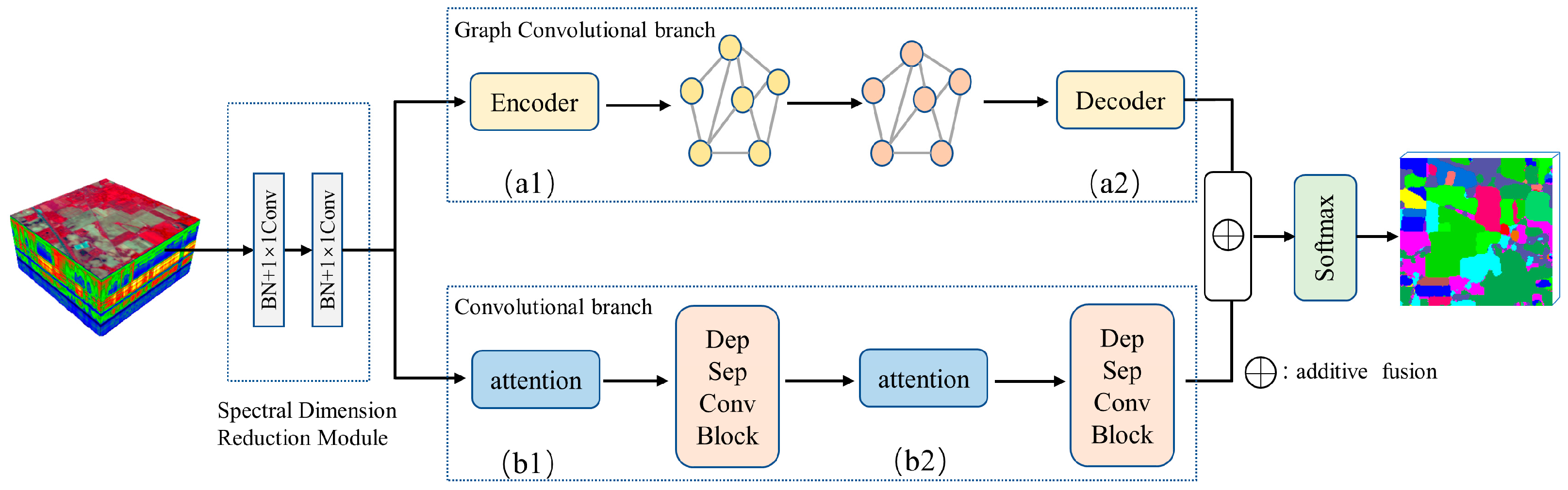
To solve the problem of missing local details in classification maps due to superpixel segmentation, we proposed a feature fusion of the CNN and GCN, as shown in Figure 1. The proposed network framework contained a spectral dimension reduction module (see Section 2.2 for details), a graph convolutional branch (see Section 2.3 for details), a convolutional branch (see Section 2.4 for details), a feature fusion module, and a Softmax classifier. It should be noted that the features extracted from convolutional neural networks were different from those of graph convolutional networks. Feature fusion methods can utilize different features of an image to complement each other’s strengths, thus obtaining more robust and accurate results. Because of that, it is possible to obtain better classification results than a single branch by fusing features from two branches.
The original HSI was handled by the spectral dimensionality reduction module first, which was used for spectral information transformation and feature dimensionality reduction. Then, we used convolutional neural networks to extract the detailed features in a local fine region. Considering the problem that the CNN-based method may induce overfitting with too many parameters and an insufficient number of training samples, we used a depth-wise separable convolution to reduce the parameters and enhance the robustness. To further improve the model, we added attention modules to the convolution branch. We used the SE attention module to optimize the proposed network [30]. The SE module can obtain the weight matrix of different channels. Then, the weight values of each channel calculated by the SE module were multiplied with the two-dimensional matrix of the corresponding channel of the original feature map. We used graph convolutional networks to extract the superpixel-level contextual features. In this branch, we applied a graph encoder and a graph decoder to implement the transformation of pixel features and superpixel-level features (see Section 2.5 for details). Next, the different features acquired by the two branches were fused to obtain richer image features by complementing their strengths. Finally, after the processing of the Softmax classifier, we obtained the label of each pixel. The role of Softmax is to assign a probability value to each output classification, indicating the probability of belonging to each class.

2.2. Spectral Dimension Reduction Module

There is a significant amount of redundant information in the original hyperspectral image. Using dimension reduction modules, it is possible to significantly reduce the computational cost without significant performance loss. The 1 × 1 convolutional layer has the ability to remove useless spectral information and increase nonlinear characteristics. Moreover, it is usually used as a dimension reduction module to remove computational cost, as shown in Figure 2. In the FCGN network, hyperspectral images are first processed using two 1 × 1 convolutional blocks. Specifically, each 1 × 1 convolutional block contains a BN layer, a 1 × 1 convolution layer, and an activation function layer. The role of the BN layer is to accelerate the convergence of the network, and the activation function layer can significantly increase the network’s nonlinearity to achieve better expressiveness. The activation function in this module adopts Leaky ReLU.
We have:
X h , w , n * = σ ( x , y , b W x , y , b , n X ˜ h , w , b + B x , y , b , n )
where X h , w , b denotes the input feature map, X ˜ h , w , b denotes the batch-normalized input feature map, X h , w , n * denotes the output feature map, W x , y , b , n denotes the convolution kernel of the input feature map in row x and column y, B x , y , b , n denotes bias, and n is the number of convolution kernels. σ represents the Leaky ReLU activation function.

2.3. Graph Convolution Branch

Numerous studies have shown that the classification accuracy can be effectively improved by combining the different features of images. Traditional CNN models can only convolve images in regular image regions using convolution kernels of a fixed size and weight, resulting in an inability to obtain global features and structural features of images. Therefore, it is often required to deepen the network layer to alleviate this problem. However, as the number of network layers deepens, the chance of overfitting increases subsequently, especially when processing data with a small amount of training samples such as HSIs. Such a result is unacceptable to us.
Therefore, a GCN branch based on superpixel segmentation was constructed to obtain the structural features. Different from the CNN, the GCN is a method used for the graph structure. The GCN branch can extract the structure features and dependency relationship between the nodes from images. These features are different from the neighborhood spatial features in a local fine region extracted by the CNN branch. Finally, the property of the network can be enhanced by fusing the different features extracted from the two branches. The graph structure is a non-Euclidean structure that can be defined as G = ( V , E ) , where V is the set of nodes and E is the set of edges. V and E are usually encoded into a degree matrix D and node matrix A, where D records the relationship between each pixel of the hyperspectral image and A denotes the number of edges associated with each node.
Because the degree of each graph node in the graph structure is not the same, the GCN cannot directly use the same-size local graph convolution kernel for all nodes similar to the CNN. Considering that the convolution in the spatial domain is equivalent to the product in the frequency domain, researchers hope to implement the convolution operation on topological graphs with the help of the theory of graph spectra, and they have proposed the frequency domain graph convolution method [31]. The Laplacian matrix of the graph structure is defined as L = D A . The symmetric normalized Laplacian matrix is defined as:
L = I N D 1 / 2 A D 1 / 2
The graph convolution operation can be expressed by Equation (3).
g θ x = U g θ Λ U T x
where U is the orthogonal matrix composed of the feature vectors of the Laplacian matrix L by column, and g θ Λ is a diagonal matrix consisting of parameter θ , representing the parameter to be learned. The above is the general form of graph convolution, but Equation (3) is computationally intensive because the complexity of the eigenvector matrix U is O ( N 2 ) . Therefore, Hammond et al. [32] showed that this process can be obtained by fitting a Chebyshev polynomial, as in Equation (4).
g θ x = k = 0 K θ k T k L ˜ x
where L ˜ = 2 λ max L I N and λ max are the largest eigenvalues of L . θ k is the vector of the Chebyshev coefficients. In order to reduce the computational effort, the literature [33] only calculates up to K = 1. λ max is approximated as two; then, we have:
g θ x θ I N + D 1 / 2 A D 1 / 2 x
In addition, self-normalization is introduced:
I N + D 1 / 2 A D 1 / 2 D ˜ 1 / 2 A ˜ D ˜ 1 / 2
where A ˜ = A + I N , D ˜ i i = j A ˜ i j . Finally, the graph convolution is:
H l + 1 = σ D ˜ 1 / 2 A ˜ D ˜ 1 / 2 H l W l

2.4. SE Attention Mechanism

The attention mechanism can filter key information from the input images and enhance the accuracy of the model with a limited computational capability. Therefore, we applied the attention mechanism to the convolutional branch. For simplicity, we chose the SE attention mechanism. The purpose of the SE module is to obtain more important feature information by a weight matrix that provides different weights to different positions of the image from the perspective of the channel domain. The SE module consists of three steps. First, the compression operation performs feature compression from the spatial dimension to turn the feature of H × W × B into a 1 × 1 × B feature. Second, the excitation operation generates weights for each feature channel by introducing the w parameter. Finally, the weight outputs from the excitation block are considered as the importance of each feature channel after selection, and the weights of each channel calculated by the SE module are multiplied with the two-dimensional matrix of the corresponding channel of the original feature map to complete the rescaling of the original features in the channel dimension to highlight the important features. The SE module is shown in Figure 3.

2.5. Superpixel Segmentation and Feature Conversion Module

The GCN can only be applied on graph-structured data, and in order to apply the GCN to hyperspectral images, the hyperspectral image needs to be constructed as a graph structure first. The simplest method is to consider each pixel of the image as each node of the graph structure, but this method leads to a huge computational cost. Therefore, it is common to first apply superpixel segmentation to the HSI.
Currently, common superpixel segmentation algorithms include SLIC [34], QuickShift [35], and Mean-Shift [36]. Among them, the SLIC algorithm assigns image pixels to the nearest clustering centers to form superpixels based on the distance and color difference between pixels. This method is computationally simple and has excellent results compared with other segmentation methods.
In general, the SLIC algorithm has only one parameter: the number of superpixels K. Suppose an image with M pixel is expected to be partitioned into K superpixel blocks; then, each superpixel block contains M/K pixels. Under the assumption that the length and width of each superpixel block are uniformly distributed, the length and width of each superpixel block can be defined as S, S = sqrt (M/K).
Second, in order to avoid the seed points falling on noisy points or line edges of the image and thus affecting the segmentation results, the positions of the seed points are also adjusted by recalculating the gradient values of the pixel points in the 3 × 3 neighborhood of each seed point and setting the new seed point to the minimum gradient in that neighborhood.
Finally, the new clustering centers are calculated iteratively by clustering. The pixel points in the 2S × 2S region around the centroid of each superpixel block are traversed. After that, each pixel is divided into the superpixel blocks closest to it; thus, an iteration is completed. The coordinates of the centroid of each superpixel block are recalculated and iterated, and convergence is usually completed in 10 iterations. Figure 4 represents the diagram of different number of superpixels in a image.
In this paper, the number of superpixel was not the same in each dataset but rather varied according to the total number of pixels in the dataset, for which the number of superpixels is specified as K = ( H × W ) / β , where H and W are the length and width of the dataset, and β is a segmentation factor to control the number of superpixels, which is 100 in this paper.
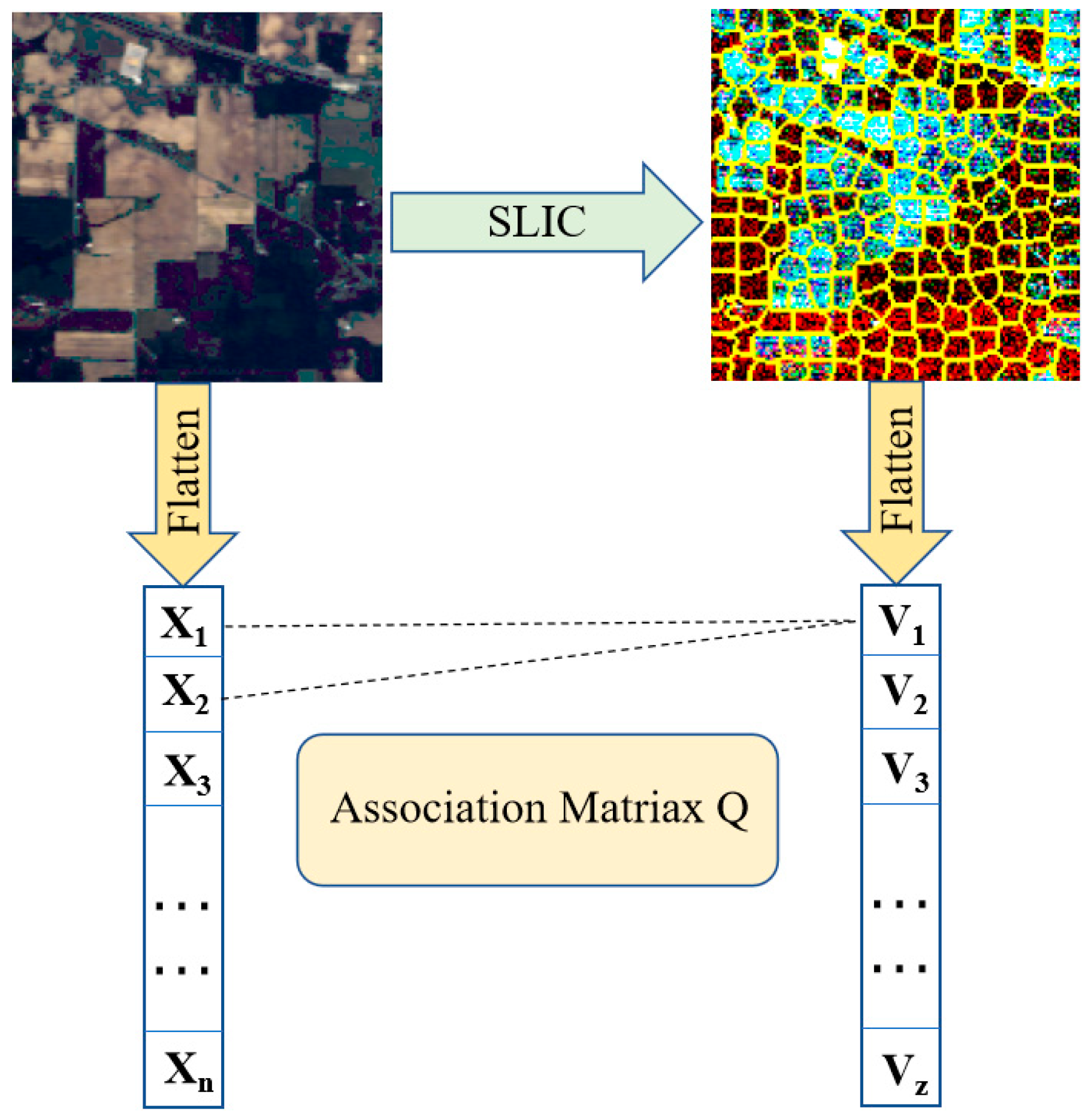
It is worth noting that since each superpixel had a different number of pixels, and because the data structures of the two branches were different, the CNN branch and the GCN branch could not be fused directly. Inspired by [28], we applied a data transformation module that allowed the features obtained from the GCN branch to be fused with the features from the CNN branch, as shown in Figure 5.
X i denotes the i-th pixel in the flattened HSI and V j denotes the average radiance of the pixels contained in the superpixels S j . Let Q R H W × Z be the association matrix between pixels and superpixels, where Z denotes the number of superpixels; then, we have:
Q i , j = 1 ,   if   X ¯ i S j 0 ,   if   X ¯ i S j ,
where X ¯ = Flatten ( X ) , Q i , j denotes the value of Q at the association matrix, and X ¯ i denotes the i-th pixel in X ¯ . Finally, the feature conversion process can be represented by:
V = E n c o d e r ( X ; Q ) = Q ^ T flatten ( X ) ,
X = D e c o d e r V ; Q = reshape Q V ,
where Q ^ denotes the normalized Q by column, and reshape Q V denotes restoring the spatial dimension of the flattened data. V denotes the nodes composed of superpixels and X denotes the feature converted back to Euclidean domains. In summary, features can be projected from the image space to the graph space using the graph encoder. Accordingly, the graph decoder can assign node features to pixels.

3. Experiments and Discussion

The overall accuracy (OA), average accuracy (AA), and kappa coefficient (kappa) were employed as the evaluation indices of the classification performance. The AA is equal to the sum of the number of correctly classified samples divided by the total number of samples. AA represents the average value of each accuracy for each category. The kappa coefficient is a reference metric that enables the calculation of overall consistency and classification consistency.

3.1. Experimental Datasets

To evaluate the effectiveness of the model, three commonly used hyperspectral datasets—Indian Pines (IP), Pavia University (PU), and Salinas (SA)—were used to evaluate the FCGN algorithm in this paper.
The IP dataset was acquired by the Airborne Visible/Infrared Imaging Spectrometer (AVIRIS) sensor over the northwestern Indian region. This dataset contains 145 × 145 pixels with 220 spectral bands ranging from 0.4 to 2.5 µm. After removing 20 water absorption and noisy spectral bands, 200 bands were reserved for the experiment. The land cover scene consists of 16 classes with 10,366 labeled pixels. The dataset was divided into training, validation, and test sets. For this dataset, the sample size was relatively small, and the number of samples of each class was extremely unbalanced. Overall, 5%, 1%, and 94% of samples per class were randomly selected for training, validation, and testing, respectively, as presented in Table 1.
The PU dataset was captured by the reflective optics system imaging spectrometer (ROSIS) sensor at Pavia University. This dataset contains 610 × 340 pixels with 125 spectral bands ranging from 0.43 to 0.86 µm. In total, 103 bands were utilized after discarding noisy bands. There are nine land cover categories in this dataset. Overall, 0.5%, 0.5%, and 99% of samples per class were selected for training, validation, and testing, respectively, as listed in Table 2.
The SA dataset is another commonly used dataset for hyperspectral image classification. It was recorded by the AVIRIS sensor over the Salinas Valley. This dataset contains 512 × 217 pixels with 224 spectral bands, and 204 bands were utilized. There are 16 land cover categories in this dataset. Because this dataset has a larger number of samples compared with Indian Pines, 0.5% of the labeled samples were selected as the training set and the validation set, and 99% of samples per class were randomly selected for testing, as listed in Table 3.

3.2. Experimental Settings

The proposed architecture consisted of three modules. The number of layers in the spectral dimension reduction module, graph convolution branch, and convolution branch were all set to two. The spectral dimension reduction modules started with two 1 × 1 convolution layers (128 filters and 128 filters). The size of the convolution kernels in the CNN branch was set to 3 × 3 (128 and 64 filters), and the sample output dimensions in the GCN branch were set to 128 and 64. We used the Adam optimizer to train our model with a learning rate of 0.001, and the training epoch was set to 500. The number of superpixels for each dataset was set to 1/100 of the number of pixels.
The proposed algorithm is implemented in Python 3.8.12 and Pytorch1.1.0 using Python language. The hardware used for training is an i7-10750H CPU and a NVIDIA GeForce RTX 2060s GPU.

3.3. Classification Results

To verify the performance of the model, several advanced HSI classification methods were selected for comparison with this model, including 3D-CNN [37], GCN [24], MiniGCN [22], HybirdSN [18], DBDA [19], and MDGCN [27]. The number of training samples and test samples selected for each method were the same, and the hyperparameters were the same as in the original paper. The classification accuracies of the different methods on each dataset are shown in Table 4, Table 5 and Table 6 the best results in each class were bolded and the classification maps obtained by these methods are illustrated in Figure 6, Figure 7 and Figure 8; the experimental results are the average of five experiments. It is worth noting that although we have minimized the risk of data leakage, the issue may still exist and affect the classification results.
Table 4 shows the classification results of the different models on the IP dataset. The lack of training samples on the IP dataset and the imbalance in the number of samples from different categories made classification challenging, but our classification method obtained the best classification results. It can be observed that the classification accuracy obtained by the 3D-CNN was lower than other methods, which might have been due to the fact that the 3D-CNN had more parameters, but the number of training samples was small in this experiment. In addition, it did not take full advantage of the relationship information contained in the samples, which eventually led to poor classification results. HybirdSN combines 3D-CNN layers with 2D-CNN layers, which has a stronger feature representation capability by combining spatial and spectral information and a lower number of parameters, but the accuracy was still lower in the case of a small number of samples. DBDA contains two branches to obtain spatial–spectral features, respectively, and introduces the attention mechanism and eventually achieved better classification results than HybirdSN. The GCN-based classification method can generally obtain better classification results with a smaller number of samples. MiniGCN adds a convolutional branch and adopts a small batch strategy compared with GCN. MiniGCN achieved better classification results but did not take into account the different importance of different features. In contrast, the FCGN obtained the best classification results, which was greatly due to the design of two branches to obtain complementary features. The graph convolution branch based on superpixel segmentation can obtain large-scale irregular features of the image and the relationship between different nodes, reducing the classification error caused by noise. The convolutional neural network with the added attention mechanism can acquire regular image features at a small image scale and generate detailed edge features, which complements the smooth features acquired by the superpixel segmentation-based graph convolution branch to obtain better classification results on both large and small scales. The convolution branch was able to process the local fine area to obtain the detailed features of the image; due to the misclassification of pixels, the classification result of the convolution branch contained more noise. By fusing the features of the two branches, the influence of noise on the classification results was greatly reduced. In terms of running time, the FCGN had a medium running time compared to the other comparison algorithms due to the use of the depth-separable convolution algorithm.
Table 5 shows the classification results of the different models on the Pavia University dataset. It can be observed that the classification results of each algorithm slightly improved relative to those of the IP dataset, which may be because of the fewer sample classes in the PU dataset and because the number of samples in each class was similar. It is remarkable that the DBDA obtained better classification results than HybirdSN, which may have resulted from the two-branch structure of HybirdSN and the attention mechanism. The FCGN performed better than the compared methods, with an OA of 98.99%, because the FCGN could fully exploit the features of the samples. Moreover, the addition of the attention mechanism also improved the classification results. The runtime of the FCGN algorithm slightly increased compared to some comparison algorithms, but considering the competitive classification results of this algorithm and the short testing time, the increase in the runtime is worth it.
Table 6 shows the classification results of the different models on the Salinas dataset. We can see that the FCGN was superior to other methods in terms of the OA, AA, and Kappa coefficient, proving the effectiveness of the FCGN algorithm again. By observing the classification results of Grapes untrained and Vineyard untrained ground features in the Salinas dataset, the classification accuracy is relatively low; this is largely because the two ground features are mixed together. We can see from Figure 8 that the FCGN method had fewer misclassified pixels than other methods and was more accurate for classifying large-scale regions.

4. Discussion

4.1. Influence of Label Ratio

To evaluate the generalizability and robustness of the proposed FCGN and other methods, we set the number of training samples per class from 5 to 25 with an interval of 5. Figure 9 shows the OA obtained by the different methods on the three datasets. It can be observed that the proposed FCGN achieved a better classification accuracy than other methods, and the classification accuracy of each method improved as the number of training samples increased, which proves the great robustness of the proposed FCGN.

4.2. Influence of Segmentation Factor

The larger the segmentation factor, the smaller the number of superpixels; therefore, the larger the size of the superpixels, the more they can preserve larger objects and suppress more noise. Conversely, the smaller the segmentation factor, the larger the number of superpixels; therefore, the smaller the size of the segmentation map obtained, the more smaller objects which can be preserved and noise which can be contained.
In order to investigate the influence of the number of superpixel blocks on the performance of the FCGN, in this section, the segmentation coefficients were set to 50, 100, 150, and 200, and the influence of different segmentation factors on the classification accuracy of the FCGN was tested on the three datasets, as shown in Figure 10. It can be seen that the classification accuracy of the FCGN on the IP dataset decreased with the increase in the segmentation coefficients, which was due to the fact that the samples in the IP dataset were of a smaller scale. The size of the superpixel was too large, which missed the sample detail information. The OA of the PU dataset was similar when the segmentation factor was 50 and 100, and the highest accuracy was achieved when the factor was 100. The sample scale on the SA dataset was much larger, so as the size of the superpixels increased, the classification results did not decrease. Instead, more noise effects were removed, increasing the accuracy. However, when the segmentation factor reached a certain size, the classification accuracy was bound to decrease gradually. In order to prevent the classification map from being smooth and missing too much detailed information, the segmentation factor was set to 100 in this chapter.

4.3. Ablation Study

The proposed FCGN mainly contains a graph convolutional branch based on superpixel segmentation and a convolutional branch with an added attention mechanism. To further validate the contribution of the two branches, we tested the OA of the two branches on three datasets separately. In addition, we tested the impact of the attention mechanism. We can intuitively see from Table 7 that the overall classification accuracy decreased when any branch was missing, which proves that the complementary features obtained by combining the graph convolution branch and the convolution branch can indeed improve the classification performance. We can also observe that the addition of attention mechanisms resulted in some improvement in the classification results, which indicates that by adding appropriate attention mechanisms to the network, we can obtain the importance of different features and capture long-range features and high-level features to improve the classification results.

5. Conclusions

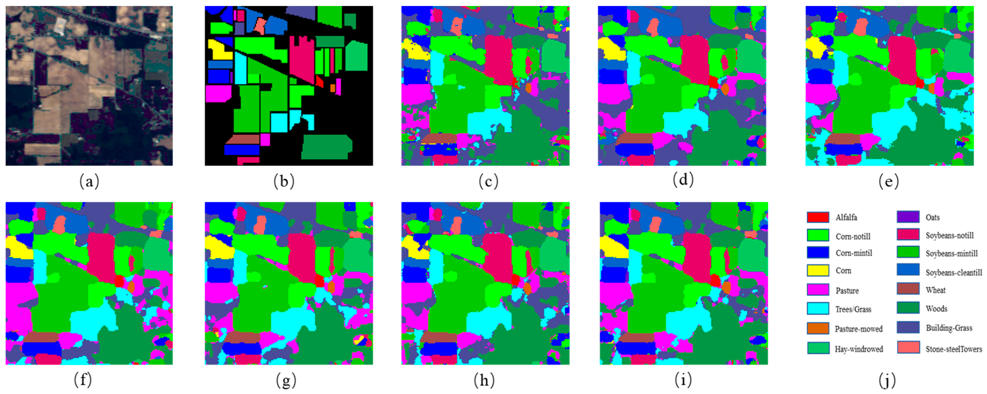
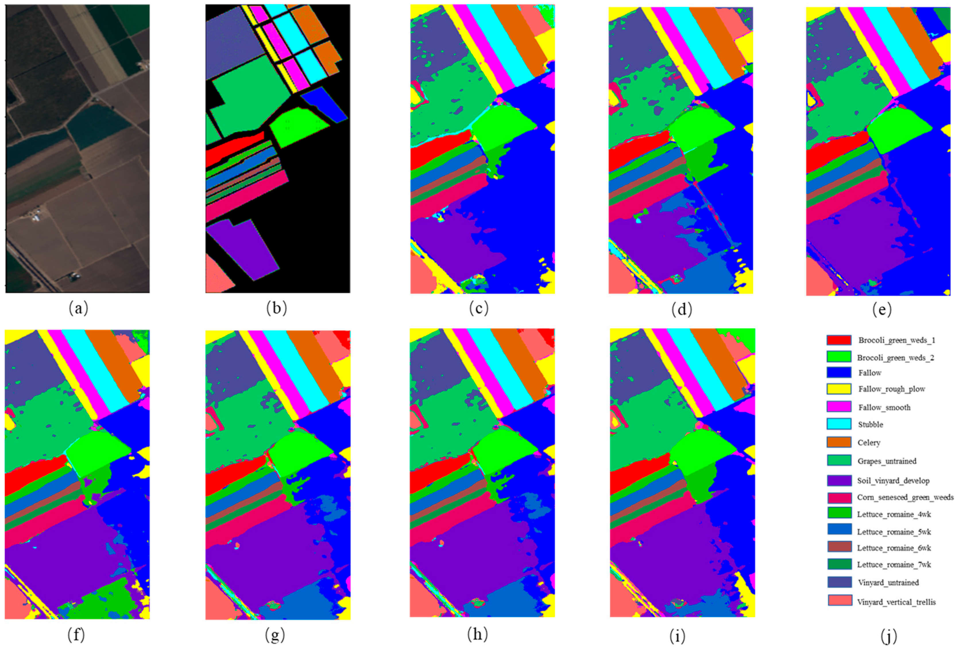
To reduce the complexity of graph structure construction, superpixel segmentation is often performed on an HSI first; however, superpixel segmentation processing leads to similar features within each superpixel node, resulting in a lack of local details in the classification map. To solve the above problems, a new hyperspectral image classification algorithm, the FCGN, was proposed in this paper, in which a graph convolutional network based on superpixel segmentation was fused with an attentional convolutional network for feature fusion, a GCN based on superpixel segmentation was used to extract superpixel-level features, an attentional convolutional network was used to extract local detail features, and, finally, the obtained complementary features were used to improve the classification results. In order to verify the effectiveness of the algorithm, experiments were conducted on three datasets and compared with some excellent algorithms. The experimental results show that the FCGN achieved a better classification performance. Although the FCGN achieved better classification results, there are still some shortcomings. In particular, this paper did not consider the variability of different neighbor nodes during the construction of the graph structure which may limit the ability of the model. In addition, only a simple feature splicing fusion method was used in this paper, so the construction of the graph structure and new fusion mechanism will be further explored in subsequent research.

Author Contributions

Conceptualization, L.G.; methodology, L.G.; software, L.G.; validation, L.G., S.X. and C.H.; formal analysis, L.G.; investigation, L.G.; resources, L.G., S.X. and C.H.; data curation, L.G.; writing—original draft preparation, L.G.; writing—review and editing, L.G. and Y.Y.; visualization, L.G. and S.X.; supervision, C.H. and Y.Y.; project administration, C.H.; funding acquisition, C.H. and Y.Y.; All authors have read and agreed to the published version of the manuscript.

Funding

This research was funded by Advanced technology industrialization of science and technology cooperation between Jilin Province and Chinese Academy of Sciences (grant number 2020SYHZ0028).

Data Availability Statement

Indian Pines dataset, Pavia University dataset, Salinas dataset (https://www.ehu.eus/ccwintco/index.php/Hyperspectral_Remote_Sensing_Scenes, accessed on 11 June 2022).

Conflicts of Interest

The authors declare no conflict of interest.

References

  1. Paoletti, M.E.; Haut, J.M.; Plaza, J.; Plaza, A. Deep Learning Classifiers for Hyperspectral Imaging: A Review. ISPRS J. Photogramm. Remote Sens. 2019, 158, 279–317. [Google Scholar] [CrossRef]
  2. Fauvel, M.; Tarabalka, Y.; Benediktsson, J.A.; Chanussot, J.; Tilton, J.C. Advances in Spectral-Spatial Classification of Hyperspectral Images. Proc. IEEE 2013, 101, 652–675. [Google Scholar] [CrossRef] [Green Version]
  3. Ma, Z.; Jiang, Z.; Zhang, H. Hyperspectral Image Classification Using Feature Fusion Hypergraph Convolution Neural Network. IEEE Trans. Geosci. Remote Sens. 2021, 60, 5517314. [Google Scholar] [CrossRef]
  4. Pan, B.; Xu, X.; Shi, Z.; Zhang, N.; Luo, H.; Lan, X. DSSNet: A Simple Dilated Semantic Segmentation Network for Hyperspectral Imagery Classification. IEEE Geosci. Remote Sens. Lett. 2020, 17, 1968–1972. [Google Scholar] [CrossRef]
  5. Tan, Y.; Lu, L.; Bruzzone, L.; Guan, R.; Chang, Z.; Yang, C. Hyperspectral Band Selection for Lithologic Discrimination and Geological Mapping. IEEE J. Sel. Top. Appl. Earth Obs. Remote Sens. 2020, 13, 471–486. [Google Scholar] [CrossRef]
  6. Dong, Y.; Liang, T.; Zhang, Y.; Du, B. Spectral–Spatial Weighted Kernel Manifold Embedded Distribution Alignment for Remote Sensing Image Classification. IEEE Trans. Cybern. 2021, 51, 3185–3197. [Google Scholar] [CrossRef]
  7. Wu, P.; Cui, Z.; Gan, Z.; Liu, F. Three-Dimensional ResNeXt Network Using Feature Fusion and Label Smoothing for Hyperspectral Image Classification. Sensors 2020, 20, 1652. [Google Scholar] [CrossRef] [Green Version]
  8. Farooque, G.; Xiao, L.; Yang, J.; Sargano, A.B. Hyperspectral Image Classification via a Novel Spectral–Spatial 3D ConvLSTM-CNN. Remote Sens. 2021, 13, 4348. [Google Scholar] [CrossRef]
  9. Peng, J.; Zhou, Y.; Chen, C.L.P. Region-Kernel-Based Support Vector Machines for Hyperspectral Image Classification. IEEE Trans. Geosci. Remote Sens. 2015, 53, 4810–4824. [Google Scholar] [CrossRef]
  10. Belgiu, M.; Drăguţ, L. Random Forest in Remote Sensing: A Review of Applications and Future Directions. ISPRS J. Photogramm. Remote Sens. 2016, 114, 24–31. [Google Scholar] [CrossRef]
  11. Zhang, M.-L.; Zhou, Z.-H. ML-KNN: A Lazy Learning Approach to Multi-Label Learning. Pattern Recognit. 2007, 40, 2038–2048. [Google Scholar] [CrossRef] [Green Version]
  12. Rish, I. An Empirical Study of the Naive Bayes Classifier. In Proceedings of the IJCAI 2001 Workshop on Empirical Methods in Artificial Intelligence, Seattle, WA, USA, 4 August 2001; Volume 3, pp. 41–46. [Google Scholar]
  13. Wan, A.; Dunlap, L.; Ho, D.; Yin, J.; Lee, S.; Jin, H.; Petryk, S.; Bargal, S.A.; Gonzalez, J.E. NBDT: Neural-Backed Decision Trees. arXiv 2020. [Google Scholar] [CrossRef]
  14. Audebert, N.; Le Saux, B.; Lefevre, S. Deep Learning for Classification of Hyperspectral Data: A Comparative Review. IEEE Geosci. Remote Sens. Mag. 2019, 7, 159–173. [Google Scholar] [CrossRef] [Green Version]
  15. Paoletti, M.E.; Haut, J.M.; Plaza, J.; Plaza, A. A New Deep Convolutional Neural Network for Fast Hyperspectral Image Classification. ISPRS J. Photogramm. Remote Sens. 2018, 145, 120–147. [Google Scholar] [CrossRef]
  16. Acción, Á.; Argüello, F.; Heras, D.B. Dual-Window Superpixel Data Augmentation for Hyperspectral Image Classification. Appl. Sci. 2020, 10, 8833. [Google Scholar] [CrossRef]
  17. Hu, W.; Huang, Y.; Wei, L.; Zhang, F.; Li, H. Deep Convolutional Neural Networks for Hyperspectral Image Classification. J. Sens. 2015, 2015, e258619. [Google Scholar] [CrossRef] [Green Version]
  18. Roy, S.K.; Krishna, G.; Dubey, S.R.; Chaudhuri, B.B. HybridSN: Exploring 3-D–2-D CNN Feature Hierarchy for Hyperspectral Image Classification. IEEE Geosci. Remote Sens. Lett. 2020, 17, 277–281. [Google Scholar] [CrossRef] [Green Version]
  19. Li, R.; Zheng, S.; Duan, C.; Yang, Y.; Wang, X. Classification of Hyperspectral Image Based on Double-Branch Dual-Attention Mechanism Network. Remote Sens. 2020, 12, 582. [Google Scholar] [CrossRef] [Green Version]
  20. Zhong, Z.; Li, J.; Luo, Z.; Chapman, M. Spectral–Spatial Residual Network for Hyperspectral Image Classification: A 3-D Deep Learning Framework. IEEE Trans. Geosci. Remote Sens. 2018, 56, 847–858. [Google Scholar] [CrossRef]
  21. Wang, L.; Wang, X. Dual-Coupled CNN-GCN-Based Classification for Hyperspectral and LiDAR Data. Sensors 2022, 22, 5735. [Google Scholar] [CrossRef]
  22. Hong, D.; Gao, L.; Yao, J.; Zhang, B.; Plaza, A.; Chanussot, J. Graph Convolutional Networks for Hyperspectral Image Classification. IEEE Trans. Geosci. Remote Sens. 2021, 59, 5966–5978. [Google Scholar] [CrossRef]
  23. Wu, Z.; Pan, S.; Chen, F.; Long, G.; Zhang, C.; Philip, S.Y. A Comprehensive Survey on Graph Neural Networks. IEEE Trans. Neural Netw. Learn. Syst. 2020, 32, 4–24. [Google Scholar] [CrossRef] [Green Version]
  24. Kipf, T.; Welling, M. Semi-Supervised Classification with Graph Convolutional Networks. arXiv 2017. [Google Scholar] [CrossRef]
  25. Full Article: Graph Inductive Learning Method for Small Sample Classification of Hyperspectral Remote Sensing Images. Available online: https://www.tandfonline.com/doi/full/10.1080/22797254.2021.1901064 (accessed on 28 January 2023).
  26. Yu, W.; Wan, S.; Li, G.; Yang, J.; Gong, C. Hyperspectral Image Classification With Contrastive Graph Convolutional Network. IEEE Trans. Geosci. Remote Sens. 2023, 61, 5503015. [Google Scholar] [CrossRef]
  27. Wan, S.; Gong, C.; Zhong, P.; Du, B.; Zhang, L.; Yang, J. Multiscale Dynamic Graph Convolutional Network for Hyperspectral Image Classification. IEEE Trans. Geosci. Remote Sens. 2020, 58, 3162–3177. [Google Scholar] [CrossRef] [Green Version]
  28. Liu, Q.; Xiao, L.; Yang, J.; Wei, Z. CNN-Enhanced Graph Convolutional Network With Pixel- and Superpixel-Level Feature Fusion for Hyperspectral Image Classification. IEEE Trans. Geosci. Remote Sens. 2021, 59, 8657–8671. [Google Scholar] [CrossRef]
  29. Chollet, F. Xception: Deep Learning with Depthwise Separable Convolutions. In Proceedings of the 2017 IEEE Conference on Computer Vision and Pattern Recognition (CVPR), Honolulu, HI, USA, 21–26 July 2017; pp. 1800–1807. [Google Scholar]
  30. Hu, J.; Shen, L.; Sun, G. Squeeze-and-Excitation Networks. In Proceedings of the 2018 IEEE/CVF Conference on Computer Vision and Pattern Recognition, Salt Lake City, UT, USA, 18–23 June 2018; pp. 7132–7141. [Google Scholar]
  31. Shuman, D.I.; Narang, S.K.; Frossard, P.; Ortega, A.; Vandergheynst, P. The Emerging Field of Signal Processing on Graphs: Extending High-Dimensional Data Analysis to Networks and Other Irregular Domains. IEEE Signal Process. Mag. 2013, 30, 83–98. [Google Scholar] [CrossRef] [Green Version]
  32. Hammond, D.K.; Vandergheynst, P.; Gribonval, R. Wavelets on Graphs via Spectral Graph Theory. Appl. Comput. Harmon. Anal. 2011, 30, 129–150. [Google Scholar] [CrossRef] [Green Version]
  33. Defferrard, M.; Bresson, X.; Vandergheynst, P. Convolutional Neural Networks on Graphs with Fast Localized Spectral Filtering. arXiv 2017. [Google Scholar] [CrossRef]
  34. Achanta, R.; Shaji, A.; Smith, K.; Lucchi, A.; Fua, P.; Süsstrunk, S. SLIC Superpixels Compared to State-of-the-Art Superpixel Methods. IEEE Trans. Pattern Anal. Mach. Intell. 2012, 34, 2274–2282. [Google Scholar] [CrossRef] [Green Version]
  35. Zhang, S.; Ma, Z.; Zhang, G.; Lei, T.; Zhang, R.; Cui, Y. Semantic Image Segmentation with Deep Convolutional Neural Networks and Quick Shift. Symmetry 2020, 12, 427. [Google Scholar] [CrossRef] [Green Version]
  36. Comaniciu, D.; Meer, P. Mean Shift Analysis and Applications. In Proceedings of the the Seventh IEEE International Conference on Computer Vision, Kerkyra, Greece, 20–27 September 1999; Volume 2, pp. 1197–1203. [Google Scholar]
  37. Chen, Y.; Jiang, H.; Li, C.; Jia, X.; Ghamisi, P. Deep Feature Extraction and Classification of Hyperspectral Images Based on Convolutional Neural Networks. IEEE Trans. Geosci. Remote Sens. 2016, 54, 6232–6251. [Google Scholar] [CrossRef] [Green Version]
Figure 1. The framework of the FCGN algorithm. (a1,a2) Feature conversion module; (b1,b2) SE attention module.
Applsci 13 07143 g001
Figure 2. Dimension reduction module. Each 1×1 convolution block contains the above three parts.
Applsci 13 07143 g002
Figure 3. Schematic diagram of SE attention mechanism mainly divided into two operations of squeeze and excitation.
Applsci 13 07143 g003
Figure 4. Schematic diagram of different number of superpixels for one image.
Applsci 13 07143 g004
Figure 5. Pixel and superpixel data conversion module. This module allows features to be propagated between pixels and superpixels.
Applsci 13 07143 g005
Figure 6. The classification maps for Indian Pines. (a) False-color image; (b) ground truth; (c) 3DCNN; (d) GCN; (e) MiniGCN; (f) HybirdSN; (g) DBDA; (h) MDGCN; (i) FCGN; (j) Figure legend.
Applsci 13 07143 g006
Figure 7. The classification maps for Pavia University. (a) False-color image; (b) ground truth; (c) 3DCNN; (d) GCN; (e) MiniGCN; (f) HybirdSN; (g) DBDA; (h) MDGCN; (i) FCGN; (j) Figure legend.
Applsci 13 07143 g007
Figure 8. The classification maps for Salinas. (a) False-color image; (b) ground truth; (c) 3DCNN; (d) GCN; (e) MiniGCN; (f) HybirdSN; (g) DBDA; (h) MDGCN; (i) FCGN; (j) Figure legend.
Applsci 13 07143 g008
Figure 9. The classification performance of each method with different training set ratios. (a) India Pines; (b) Pavia University; (c) Salinas.
Applsci 13 07143 g009
Figure 10. The classification performance with different segmentation factors. (a) India Pines; (b) Pavia University; (c) Salinas.
Applsci 13 07143 g010
Table 1. The dataset division for each class of the IP dataset.
NO.CLASSTrainValTest
1Alfalfa3150
2Corn-notill72141348
3Corn-mintil428784
4Corn122220
5Pasture254468
6Trees/Grass377703
7Pasture-mowed2123
8Hay-windrowed244461
9Oats1118
10Soybeans-notill489911
11Soybeans-mintill123242321
12Soybeans-cleantill316577
13Wheat112199
14Woods65121217
15Building-Grass193358
16Stone-steelTowers5189
Total520999747
Table 2. The dataset division for each class of the PU dataset.
NO.CLASSTrainValTest
1Asphalt34346563
2Meadows949418,461
3Gravel11112077
4Trees/Grass16163032
5Metalsheets771331
6Baresoil26264977
7Bitumen771316
8Bricks19193644
9Shadows55937
Total21921942,338
Table 3. The dataset division for each class of the SA dataset.
NO.CLASSTrainValTest
1Brocoli_green_weds_111111987
2Brocoli_green_weds_219193688
3Fallow10101956
4Fallow_rough_plow771380
5Fallow_smooth14142650
6Stubble20203919
7Celery18183543
8Grapes_untrained575711,157
9Soil_vinyard_develop32326139
10Corn_senesced_green_weeds17173244
11Lettuce_romaine_4wk661056
12Lettuce_romaine_5wk10101907
13Lettuce_romaine_6wk55906
14Lettuce_romaine_7wk661058
15Vinyard_untrained37377194
16Vinyard_vertical_trellis10101787
Total27927953,571
Table 4. Classification results of the IP dataset.
Class3DCNNGCNMiniGCNHybirdSNDBDAMDGCNFCGN
180.0094.6693.7383.4499.5188.88100.00
290.1670.3772.5480.3893.5596.1696.51
380.0566.8976.8382.2194.1194.1798.46
486.5486.8898.1699.1996.4292.5997.36
584.4389.2793.4096.4797.6496.7997.13
679.1293.3892.6498.8196.2399.50100.00
767.2292.9188.4886.8996.6696.8292.89
890.8796.1497.5998.0491.3595.7298.68
970.00100.0099.7373.1189.3799.98100.00
1079.1185.3775.9890.4170.3085.7097.30
1190.8168.4579.4274.2390.3296.0698.63
1272.5078.9079.5191.0097.3898.8895.17
1370.8899.8498.9371.8897.9997.2199.59
1485.8385.1287.8898.3398.3499.9399.33
1592.3082.6789.8294.4896.2596.1795.71
1669.2297.41100.0070.2286.6694.8297.75
OA(%)78.4786.6788.6787.9994.5597.6298.78
AA(%)80.5786.7789.0486.8293.2695.5897.80
Kappa80.7084.3888.3987.4494.0195.4997.99
Train time(s)250.1159.02342.55220.99298.321204.15204.50
Test time(s)15.045.6015.3814.5121.7720.335.92
Table 5. Classification results of the PU dataset.
Class3DCNNGCNMiniGCNHybirdSNDBDAMDGCNFCGN
180.8577.2686.2294.1096.3699.0098.41
280.4976.9792.2194.3699.1198.2199.91
369.7769.1986.1382.4090.3286.8197.35
495.9990.8892.0695.2797.9994.5597.96
591.3094.2795.1195.7799.0199.7699.73
690.5792.9890.3492.4497.5599.8099.00
780.2182.8188.9989.0694.3798.0799.89
889.7386.9182.7780.0488.9496.9298.68
991.1295.5592.8799.1198.3998.3898.41
OA(%)86.3385.4189.6792.9997.2298.2298.99
AA(%)85.5685.2089.6392.8195.7896.8398.81
Kappa85.2180.3787.0989.9896.7297.2797.90
Train time(s)131.44251.591058.37122.61145.883265.311283.37
Test time(s)88.2117.3350.1565.48118.3757.2938.94
Table 6. Classification results of the SA dataset.
Class3DCNNGCNMiniGCNHybirdSNDBDAMDGCNFCGN
188.3198.6496.1999.3499.62100.0099.74
288.3598.9999.0298.6199.14100.00100.00
382.0173.8486.3294.3897.4599.16100.00
484.0299.4998.3297.0494.77100.0099.82
587.7699.6696.3598.2498.0294.3297.71
691.4299.9799.5599.0399.9999.9898.98
790.9493.5498.5496.8997.6298.8599.99
880.0794.7091.4086.5587.3586.1894.25
994.88100.0099.7499.1289.3799.9799.97
1088.7670.8284.2589.8989.5793.8496.68
1183.6280.8583.5191.2390.3298.2999.01
1287.9995.0594.9997.9297.3894.9899.99
1372.1594.9489.4799.4698.9997.0099.36
1473.0597.8298.9497.6695.6997.1299.10
1591.3454.2567.3981.4786.7795.9294.56
1692.9665.6064.6199.2896.3498.6598.67
OA(%)86.3091.4791.7696.2592.5596.8098.69
AA(%)86.1090.9290.5395.3894.9097.1498.61
Kappa85.0988.0188.3992.0993.3795.3497.18
Train time(s)153.09269.041094.67146.96176.553377.411357.15
Test time(s)93.3723.0257.4772.72120.1765.3342.46
Table 7. OA(%) indices of the ablation experiment of the FCGN.
DatasetBranch1Branch2Without SEFCGN
Indian Pines93.5894.6996.4498.78
Pavia University95.6593.4197.9898.99
Salinas97.3394.5097.8898.69
Disclaimer/Publisher’s Note: The statements, opinions and data contained in all publications are solely those of the individual author(s) and contributor(s) and not of MDPI and/or the editor(s). MDPI and/or the editor(s) disclaim responsibility for any injury to people or property resulting from any ideas, methods, instructions or products referred to in the content.

