Abstract
Analyzing land use changes (LUC) in both past and future scenarios is critical to optimize local ecology and formulate policies for sustainable development. We analyzed LUC characteristics in Huaibei City, China from 1985 to 2020, and used the CLUE-S and PLUS models to simulate LU in 2020. Then, we compared the accuracy of the simulation phase and chose the PLUS model to project LU under four scenarios in 2025. The results showed the following: (1) Farmland and grassland areas decreased from 1985 to 2020, while forestland, water, and construction land increased. (2) The LU types in the region are explained well by the driving factors, with all receiver operation characteristic (ROC) values greater than 0.8. (3) The kappa indices for CLUE-S and PLUS analog modeling were 0.727 and 0.759, respectively, with figure of merit (FOM) values of 0.109 and 0.201. (4) Under the farmland and ecological protection scenario (FEP), farmland and forestland areas are protected, increasing by 1727.91 hm2 and 86.22 hm2, respectively, while construction land decreases by 2001.96 hm2. These results confirm that PLUS is significantly better than the CLUE-S model in modeling forestland and water, and slightly better than the CLUE-S model in modeling the rest of the LU type. Urban sustainability is strong in the scenario FEP.
1. Introduction
As an important component and major cause of global environmental change, land use/land cover change (LUCC) is a manifestation of human–earth system interaction, which is driven by natural and anthropogenic factors but also directly affects the processes of material exchange and energy cycling in the hydrosphere, pedosphere, atmosphere, and biosphere [1,2,3]. While global environmental changes have been studied intensively, problems caused by LUCC have been discussed and studied extensively, such as loss of farmland, water pollution, and biodiversity reduction. Therefore, exploring both historical and future scenarios of LUCs is crucial in making sensible proposals for sustainable development [4].
With the advancement of geographic information systems (GIS) and remote sensing (RS), LUC modeling has become one of the main methods to research LUC. Models are important tools for exploring LU driving factors, supporting urban planning and policy making, and assessing the ecological impact of LU [5]. Scholars now mainly use integrated models to make up for the inadequacy of separate models. Bian et al., coupled the conversion of land use and its effects (CLUE-S) model with the Markov, gray prediction, and linear regression methods, respectively, to compare the three simulation results and set two future scenarios within the Qinhuai River basin [6]. Wang et al., coupled the system dynamics (SD) model, patch-generating land use simulation (PLUS) model, and integrated valuation of ecosystem services and tradeoffs (InVSET) model to simulate the LU and carbon storage changes in Bortala based on the CMIP6 published climate change scenarios [7]. Cunha et al., predicted LUC for agricultural development in primary planted areas of the Cerrado and Atlantic woodland intersections in Brazil using CA-Markov [8]. Apart from the above models, the future land use simulation (FLUS) model [9] and agent-based model (ABM) are also common [10]. Spatial models are particularly important among the hybrid models, with different spatial models exhibiting different simulation results and differences in the suitable regions. The FLUS model allows for nondominant land class conversion and can simulate leapfrog development scenarios. However, it is difficult to clearly reflect spatial differences in land use changes in different locations. The ABM model is suitable for the dynamic simulation of policy-driven urban expansion and land use changes, but it is difficult to represent the spatial behavior of the subject [4]. The CLUE-S model is applicable to LUC research on a small scale and can simulate multiple land use changes simultaneously. It has been widely used in previous research with high simulation accuracy [11,12]. The PLUS model is improved on the basis of the FLUS model, which explains the influencing factors of LUCs well, and can better model the LU patch-level changes with high simulation accuracy [13,14]. Therefore, we compared the CLUE-S and PLUS models and chose the model that was more applicable to the region.
Huaibei City is one of the top ten coal bases in China. For many years, the mining of coal resources has made the city pay a heavy price in terms of land sinkage, near resource depletion, and ecological degradation [15]. So, this study analyzed the LUC in Huaibei City between 1985 and 2020. The CLUE-S model and PLUS model were selected to simulate the spatial landscape of LU in 2020. Simulation results of the two models are compared to explore possible future scenarios and support decision making for the future.
2. Materials and Methods
2.1. Study Area
Huaibei City is located in the northern part of Anhui Province, eastern China (116°23′~117°23′ E, 33°16′~34°14′ N), as described in Figure 1. The study area covers 726.52 km2. The topography inclines from NW to SE, and the rest is a vast plain except for a small amount of low mountainous terrain in the NE. The mineral resources of Huaibei City are relatively abundant, mainly coal and other nonmetallic minerals; a small number of metal minerals are also available. By 2015, 56 coal mining sites were identified, with coal reserves of 5.633 billion tons. The accumulated coal-mining-collapsed land in Huaibei City is 228.00 km2, the new collapsed land is 4.3~4.5 km2 every year, and the reclaimed collapsed land area is 121.40 km2 [16].
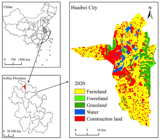
Figure 1.
Geographical location of Huaibei City in China.
2.2. Data Source and Processing
The sources and related descriptions of the study data are presented in Table 1, where natural environmental data and socioeconomic data were used as driving factors for the LU simulation: (1) LU data of Huaibei City for 1985, 1995, 2005, 2015, and 2020. The 2015 LU data were obtained from Landsat8 OLI image interpretation of Geospatial Data Cloud (http://www.gscloud.cn, accessed on 27 June 2022). Based on the LU classification of the Chinese Academy of Sciences, LU data were classified into five major classes: farmland, forestland, grassland, water, and construction land. (2) The 16 driving factors that can work on LUC were chosen in this study based on the selection principles [17]. These include the digital elevation model (DEM), aspect, slope, distance from the railroad (Railway_d), distance from the freeway (Freeway_d), distance from the roads (Road_d), distance from the rivers (River_d), distance from towns (Town_d), soil organic matter (Soil_SOM), total nitrogen (Soil_TN), total phosphorus (Soil_TP), total potassium (Soil_TK), gross domestic product (GDP), population density (POP), mean annual temperature (MAT), and mean annual precipitation (MAP). Figure 2 shows the driving factors after the normalization process. (3) Soil data were obtained from the soil sample datasets obtained from the 2010–2011 soil surveys, including soil organic matter, total nitrogen, total phosphorus, and total potassium data. The sample points are linked to the vector map according to the same soil type and transformed into a raster. (4) The slope and aspect data were extracted from DEM in ArcGIS. (5) Spatial distance driving factor maps from railroads, freeways, roads, rivers, and towns were gained from vector data acquired from Open Street Map by performing Euclidean distance analysis in ArcGIS.

Table 1.
Data source information of the research.
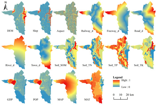
Figure 2.
Driving factors.
2.3. Research Methodology
2.3.1. Markov Model
A stochastic process is said to have Markovianity (no posteriority) if the state an of any moment tn in a finite time sequence t1 < t2 < t3…tn is only related to the state an−1 of its predecessor tn−1; the process with Markovianity is called a Markovian process. The LULC change process can be viewed as a Markov process [18]. Therefore, variations in the area of LU types can be predicted using the following equation:
where S(t) and S(t+1) represent the states of the LU system at moments t, t + 1, respectively; Pij is the state transfer matrix.
2.3.2. CLUE-S Model
The CLUE-S model is an improved model for small regions based on the CLUE model by Verburg et al., of Wageningen University in the Netherlands. Within the CLUE-S model, a raster is used as the study unit, and the LU type on the raster indicates the LU status [19,20,21]. The CLUE-S model consists of nonspatial and spatial analysis modules. The nonspatial module is based on the analysis of natural, social, economic, and policy driving factors of LUC, and other models or methods are used to calculate the LU demand for each simulation year; the Markov model is chosen to calculate the land demand data in this study.
In the CLUE-S model, the development probability of each type of LU needs to be found using a logistic regression equation; the auto-logistic model, which uses neighborhood correlation to construct spatial autocorrelation weights, has better predictive ability than the general logistic model in finding the development probability of each LU type. The auto-logistic equation was first proposed by Besag [22] and the general expression is as follows:
where X represents a vector consisting of a set of driving factors; yi represents the state of the event as a binary variable; and wij represents the spatial weight value.
In this study, the weight matrix is constructed with the help of neighborhood factors, and the spatial weights are set as [23,24]
where Sjn is the similarity of each neighboring raster around raster j to j, with 1 for the same LU type and 0 otherwise, and N is the total number of neighbors of neighboring raster j. To test the effect of regression analysis, the receiver operation characteristic (ROC) method can be used to evaluate the driving factor for the explanatory ability of each type. Generally, it is considered that the ROC is greater than 0.7, which indicates that the driving factor has a good explanatory ability for the type [25].
2.3.3. PLUS Model
The PLUS model is a type of CA-based patch generation LUC model. This model allows excavation of the driving factors of land sprawl and changes in the landscape to better model the generation and variation of LU patches [26,27,28,29]. In PLUS, the Land Expansion Analysis Strategy (LEAS) module excavates the driving factors and expansion factors. Then, the development probability of each LU type and the contribution of the driving factors to land expansion is calculated. The CA based on the multiple-type random patch seeds (CARSs) module incorporates random seeds and a patch generation threshold to simulate and predict the future landscape pattern under the control of development probability [30,31].
PLUS Model V1.3.5 is used in this study, with the following steps: (1) The selected LU data and driving factors need to be unified to the same projection coordinate system and resolution, and the LU data are converted to unsigned char format. (2) Extract the part of LU expansion during the period. (3) Input the LU expansion data and set various parameters in the LEAS module. The parameters of the simulation phase are as follows: the number of regression trees is 20, the sampling rate is 0.02, and the number of training features is 16. The development probability map of each LU type is acquired. (4) Finally, each parameter is input into the CARS module and debugged to achieve the simulation of future landscape patterns. The parameters are set as follows in the simulation stage: the patch generation threshold is set to 0.8, the expansion coefficient is set to 0.3, and the percentage of seeds is set to 0.0005. The Markov chain is included with the PLUS model, and the calculation of future LU demand can be conducted in the PLUS model.
2.3.4. Calibration and Validation
Three metrics were used to evaluate the model’s accuracy: (1) Kappa coefficient, calculated as follows [32,33].
where P0 is the proportion of correct simulation results; Pc is the proportion of correct simulation results expected under random conditions; and Pp is the proportion of correct simulation results under ideal conditions. In general, the consistency is high when the kappa value is greater than 0.75, the consistency averages in the range of 0.4 to 0.75, the consistency is poor when it is less than 0.4, and the simulation accuracy is poor.
(2) Figure of Merit (FOM) [34], used to verify the consistency of spatial position change; 0 means no overlap, and 1 means complete overlap. (3) User’s accuracy [35], which measures the number of pixels that the model predicts accurately as a change in the proportion of all the changes it predicts and can be used to describe the proportion of the model predicting the correctness of a certain type of LU.
3. Results
3.1. Spatial and Temporal Changes in Land Use
Calculation of the integrated LU dynamics for the four time periods from 1985 to 2020 revealed that it was 0.04% from 1985 to 1995, 2.21% from 1995 to 2005, 18.51% from 2005 to 2015, and 34.62% from 2015 to 2020. LUCs in the region were faster after 2005, which may be related to rapid socioeconomic development and accelerated urban transformation. Figure 3 shows the Sankey diagram produced by the LU transfer matrix of the study area from 1985 to 2020, indicating the transfer in and out of each LU type in different periods. From the figure: (1) From 2005 to 2015, transfers in and out between LU types were more frequent. Farmland was largely reduced and 82% of the transferred out area was transferred into construction land. The water area decreased by 12.06 km2 and the largest area was transferred to farmland and construction land. Overall, the area of construction land increased by 51.45 km2 in this period, of which 67.45 km2 of farmland was transferred to construction land, 4.19 times more than the previous time. (2) From 2015 to 2020, there are different degrees of area transfer between each LU type; the change is 164.29 km2 and the farmland continues to decrease by 27.35 km2. Additionally, the water area increased by 15.10 km2, mainly from farmland and construction land. The construction land increased by 5.88 km2 and the growth was mainly from grassland, which was transferred into 6.06 km2. In a comprehensive view of the four time periods, the area of farmland has been decreasing and the ratio of the area transferred into construction land to the total area transferred out from farmland was 86%, 83%, 82%, and 60%. The areas of other LU types transferred into water in the four time periods were 0.30 km2, 2.51 km2, 6.66 km2, and 21.50 km2, in order.
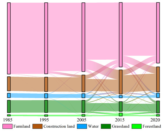
Figure 3.
Sankey diagram of LU type conversion from 1985 to 2020.
3.2. Simulation and Validation
3.2.1. Logistic Regression Analysis
Table 2 shows the β-coefficients of the results of logistic regression and auto-logistic regression. The spatial autocorrelation factor (AutoValue) in auto-logistic regression, is the spatial weight value of each LU type calculated according to Equation (3). The results show that the ROC values of auto-logistic regression analysis with AutoValue were all improved: 0.856 for farmland, 0.933 for forestland, 0.934 for grassland, 0.935 for water, and 0.829 for construction land. The ROC values are all greater than 0.8, and forestland, grassland, and water reach more than 0.9 indicating a high fitting accuracy and strong explanation ability of the selected driving factors. As shown in Table 2, the main driving factors of farmland are POP, DEM, MAP, GDP, and Town_d. The distribution of forestland is mainly influenced by Town_d, River_d, MAP, MAT, and DEM. It is most influenced by Town_d, followed by MAP. For grassland, the main driving factors affecting its distribution are DEM, MAP, River_d, Slope, and Soil_SOM. Additionally, mainly the locational factors such as River_d and Freeway_d are negatively correlated, and positively correlated with natural factors such as DEM and Slope. The driving factor affecting the water is mainly the DEM, which shows a significant negative correlation. Construction land is mainly influenced by POP, GDP, MAP, DEM, and Town_d. It is most influenced by POP and shows a significant positive correlation.
Table 2.
β value of Logistic regression and auto-logistic regression for each LU type.
3.2.2. Simulation Results of CLUE-S Model
The LU in 2015 was adopted as the base map to simulate the LU in 2020 to validate the accuracy of the CLUE-S model simulation. Firstly, the auto-logistic regression results were calculated in SPSS and saved as the alloc1.reg parameter file as requested by the CLUE-S model. Secondly, we processed the driving factors, calculated the LU demand, prepared the transfer matrix, and set the main parameters of the model. Then, we ran the CLUE-S model to obtain the simulated LU map in 2020, as shown in Figure 4a.
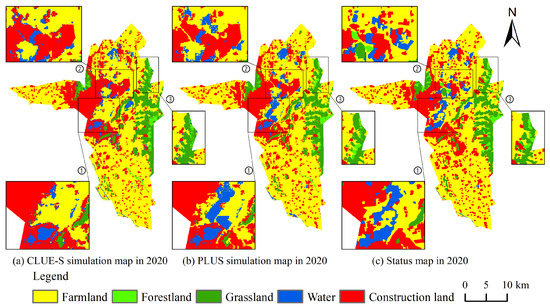
Figure 4.
Comparison of simulation results of different models in 2020.
The CLUE-S simulated map in 2020 was compared with the status map in 2020 for verification. A kappa coefficient of 0.727 can be calculated in ArcGIS based on Equation (4), indicating that the simulation is generally consistent.
3.2.3. Simulation Results of PLUS Model
In PLUS, land expansion is firstly extracted based on the 30 m resolution LU maps of 2015 and 2020. Then, the development potential of each LU type on each unit is predicted through the LEAS module, and the development potential map of each LU type is output. Finally, the LU in 2020 is simulated by setting various parameters through the CARS module, as shown in Figure 4b. The kappa coefficient is 0.759, a 0.032 improvement over the CLUE-S model, and the simulation result is better. This indicates that the PLUS model has good applicability in the study area and can be used for LU studies of future scenarios.
3.3. Comparison of CLUE-S and PLUS Simulation Results
Figure 4 shows the simulation result map of the two models and the status map in 2020 under the scale of 30 m × 30 m. Table 3 shows the area of each LU type obtained from the simulation result map. From Figure 4 and Table 3, the spatial location distribution and quantity of each LU type in the PLUS simulation map and the status map are more similar. The water area in the CLUE-S simulation is smaller than the actual status map, and areas that should be water are incorrectly modeled as farmland, as shown in local area ① in Figure 4a. Figure 4b shows that there are waters in region ①. The PLUS simulation map indicates the presence of water at this location, suggesting that the PLUS model is better able to explore potential driving factors. In the north and south where the topography is flat, the area of farmland in the CLUE-S and PLUS simulations is slightly larger than the status map, while the construction land is clustered toward the middle part, as shown in the local area ② in Figure 4. There are fewer construction land patches in the CLUE-S simulation result map than in the PLUS simulation result map, indicating that the construction land is clustered more strongly in the CLUE-S simulation result map. Furthermore, it was found that the area of farmland and construction land in the CLUE-S simulation result map was slightly more than that in the PLUS simulation result map and the status map, and the area of forestland, grassland, and water was slightly less than that in the PLUS simulation map and the status map. As shown in local area ③ of Figure 4, both models failed to simulate a portion of grassland and forestland in the northwest. Additionally, the two models were most likely to differ where the edge of the LU type was excessive. The kappa coefficients of the CLUE-S and PLUS models were calculated to be 0.727 and 0.759, and the FOM values were 0.109 and 0.201. It is easy to know that the simulation accuracy of the PLUS model is better than that of the CLUE-S model at the same scale in the study area. The user’s accuracy results of the two models are shown in Table 4, and it can be found that the accuracy of the PLUS model in simulating forestland and water is much improved than that of the CLUE-S model.
Table 3.
Areas simulated by different models of LU type in 2020 (hm2).
Table 4.
User’s accuracy of CLUE-S and PLUS models at 30 m resolution.
3.4. Multiscenario Simulation of Land Use Change in Huaibei City, 2020–2025
3.4.1. Multiple Scenario Settings
Based on the General Land Use Plan of Huaibei City (2006–2020), the Fourteenth Five-Year Plan for National Economic and Social Development of Huaibei City, and the Outline of Vision 2035, combined with the experience of previous scholars, four development scenarios were structured to study the future LU pattern of Huaibei City, including the natural growth scenario (NG), farmland protection scenario (FP), ecological protection scenario (EP), and farmland and ecological protection scenario (FEP). Changes in future LU patterns under different scenarios are predicted by modifying relevant parameters such as LU demand in the PLUS model. The LU demand from 2020 to 2025 in the scenarios is calculated by adapting the Markov transfer probabilities between LU types from 2015 to 2020.
- (1)
- NG scenario: the transfer probability from 2020 to 2025 is presumed to grow naturally according to the evolutionary trend from 2015 to 2020.
- (2)
- FP scenario: Combined with the policies on farmland in China’s LU plan and the 14th Five-Year Plan, it is necessary to keep the quantity of farmland but also to protect the quality of farmland from declining and to implement the strictest farmland protection measures. Therefore, the transfer probability matrix under the FP scenario in this study is to reduce the transfer probability of farmland to other LU types by 50% under the NG scenario, whilst other LU types still maintain the natural development trend.
- (3)
- EP scenario: Farmland is also the main part of the farmland ecosystem. Therefore, the EP scenario is set to reduce the transfer probability of farmland, forestland, grassland, and water to construction land by 30%, 50%, 20%, and 20%, respectively. The transfer probability of forestland to grassland is reduced by 50%, increasing the transfer probability of water and grassland to forestland by 20% and the transfer probability of construction land to forestland by 10% under the NG scenario.
- (4)
- FEP scenario: In China’s 14th Five-Year Plan, it is mentioned that we need to implement sustainable development and strengthen ecological protection and restoration. Therefore, a more reasonable dual protection scenario is set up by integrating the FP scenario and EP scenario. Under the transfer probability based on natural growth, the transfer probability of farmland to other LU types (except forestland) is reduced by 50%. Forestland, grassland, and water to construction land is reduced by 50%, 20%, and 20%, respectively. Forestland to grassland is reduced by 50%, water and grassland to forestland is increased by 20%, and construction land to forestland is increased by 10%. The LU demand for each scenario was calculated based on the adjusted transfer probabilities of each LU type, and Table 5 shows the LU demand in 2025 under the four scenarios.
Table 5. LU demand under different scenarios in 2025 (hm2).
3.4.2. Multiscenario Simulation under PLUS Model
The calculated future LU demand under multiple scenarios was input into the PLUS model with the status LU map in 2020 as the base map, and the remaining parameters were modified. The LU patterns of the study area in 2025 under multiple scenarios generated by the CARS module are shown in Figure 5.
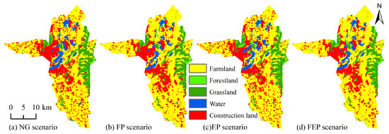
Figure 5.
PLUS simulation results of LU pattern evolution under four scenarios in Huaibei.
Farmland expansion is primarily influenced by factors such as DEM, GDP, and POP. Typically, areas that are farther away from urban centers and have relatively flat terrain are preferred for farmland expansion. The south and north of the study area meet the requirements for the expansion of farmland. Construction land is strongly influenced by economic factors, so it will be clustered toward the densely populated areas in the simulation result map. As in the scenario FEP, farmland is more in the south and north of the study area, while the construction land is clustered inward. The expansion of grassland and forestland is mainly determined by location factors, such as DEM. In general, their expansion occurs in high-elevation areas that are far from major roads. The water is mainly influenced by DEM, and its expansion generally occurs in the low-elevation area. As in the scenario EP, the transition of forestland and grassland occurs in the northwest and east of high elevation, and water occurs in the low-elevation area between two forestlands.
Under scenario NG, the spatial distribution of LU type does not differ much from the status map in 2020. The area of water increases in the central part of the study area, and the construction land continues to expand to the surrounding area. The area of farmland and forestland continues to show a decreasing trend compared with the status map in 2020. Farmland decreases by 1683.81 hm2 and forestland decreases by 301.50 hm2, which are 3.98% and 24.71%, respectively, compared to 2020. Furthermore, the area of construction land increases by 362.7 hm2, which is 2.06% compared with 2020. This indicates that the rate of loss of forestland is faster and the increase in construction land is gradually moderated under scenario NG. The reduction in farmland will lead to a threat to food security and the reduction in forestland will lead to ecological damage, thus making socioeconomic development less sustainable.
Under scenario FP, the farmland patches become larger. The patches of construction land become smaller and more compact in the middle. The largest increase in farmland is observed, with an increase of 1869.57 hm2 compared to 2020. The area of forestland is less than in the NG scenario, with a decrease of 402.66 hm2. Grassland decreases by 34.92 hm2. The water increases by 317.34 hm2 but decreases by 604.53 hm2 compared to the NG scenario. The construction land decreases by 1749.33 hm2, while grassland, water, and construction land increase under the NG scenario, indicating that most of the increase in these LU types comes from farmland.
In the EP scenario, the northwestern part of the study area is occupied by part of the construction land due to the outward expansion of water and forestland. Some grassland was also converted to forestland in the east. The EP scenario controls the loss of farmland area. The area of forestland, grassland, and water increased. Water area increased the most with 972.81 hm2 and the area of building land decreased by 1157.13 hm2.
Under scenario FEP, the construction land is clustered inward and the internal grassland is occupied. The expansion of forestland in the northwest partly encroached on the construction land. The farmland increases by 1727.91 hm2 and the forestland increased by 86.22 hm2. The construction land decreases the most by 2001.96 hm2. Under the FEP scenario, both farmland and forestland are protected, food security is guaranteed, and the ecological environment is preserved and improved. The expansion of construction land is restrained and the development sustainability of the urban is stronger compared to the NG scenario. Additionally, the area of the water is increased in all four scenarios. Table 6 below shows the area of each LU type under the four scenarios compared with the status of LU in 2020.
Table 6.
Changes of the regional area under different scenarios in 2020–2025 (hm2).
4. Discussion
This study analyzed the historical LUCs in the study area and explored the evolution process. Then, a model with high accuracy was selected to simulate future LUs. The study results can be used for regional LU planning to provide some decision support. The transformation between LU types was calculated in the study, with the conversion of farmland into construction land as the main focus; this finding is the same as that of the previous research on Huaibei City [36]. The study area showed a continuous increase in the area of construction land and a decrease in the total area of farmland; the results of this study are the same as the findings of Li et al., in that farmland shows a gradual decrease trend and construction land shows a gradual increase trend [37]. Among the driving factors with strong explanatory power for farmland are POP, DEM, MAP, GDP, Town_d, etc., which is similar to the results of previous studies [38]. The driving factors with stronger explanatory power for construction land are mainly the POP, GDP, MAP, DEM, etc., which are dominated by socioeconomic factors, which is similar to the findings of Zhao et al. [21]. Forestland and grassland are mainly influenced by natural driving factors, such as River_d, DEM, MAP, etc. The driving factor with the strongest explanatory power for water was DEM; similar conclusions were reached by previous authors, and the results of Zhang et al., showed that slop was the main expansion factor affecting grassland, followed by MAP, and the highest driving factors affecting the expansion of water were elevation, population density, and distance to the water system [39]. Both the improved CLUE-S model and the PLUS model have their advantages. The improved CLUE-S model incorporates spatial autocorrelation factors, which can enhance the overall accuracy of the model simulation [40]. In contrast, the newly developed PLUS model, can explore potential driving factors and better simulate LUCs at the patch level to obtain better simulation accuracy. The comparison of the simulation results of CLUE-S and PLUS models in the study area revealed that the PLUS model outperforms the improved CLUE-S model in terms of spatial location distribution and quantity at the same scale resolution, especially in the simulation of ecological LU types. Moreover, the accuracy of the PLUS model is better at fine resolution, while the CLUE-S model is not. The CLUE-S model has similar accuracy to PLUS in simulating construction land and farmland, but the area of simulation results will be greater than in the PLUS model. Similar conclusions have been drawn from earlier studies. Jiang et al., showed that the PLUS model outperformed the CLUE-S model in spatial location distribution and quantity prediction, and the CLUE-S model had higher simulation accuracy in flat terrain areas [41].
Bian et al., set up comprehensive scenarios based on different policy requirements as well as economic development and environmental protection needs [6]. Wang et al., set up scenarios SSP126, SSP245, and SSP585 based on the SSP-RCP scenarios provided by CMIP6. Therefore, future scenarios need to be set up using local realities [7]. The current planning of Huaibei City, which is transformed by the resource city, has shown problems such as lagging strategic LU targets, ecological and farmland protection to be upgraded, and unreasonable spatial layout of the landscape. These problems are inconsistent with the fast-developing socioeconomic environment, and the planning needs to be adjusted and perfected promptly [42]. The four scenarios set in this context can provide an understanding of the evolutionary trends of LU patterns in the future. Among the four future scenarios, farmland and forestland continue to decrease with conversion to construction land under scenario NG, which does not meet the relevant planning requirements; future over-expansion of construction land will, therefore, need to be curbed [43]. The FEP scenario restrains the growth of construction land and protects ecological land and farmland. The occupation of farmland and forestland will be controlled basically in the future with the delineation of the three control lines. However, due to the high degree of LU in Huaibei City and the need to protect the demand for new urbanization land, conflicts between supply and demand for construction land may arise in a short period. For this reason, scientific and reasonable planning of the land spatial distribution is needed in future development in conjunction with the current situation to improve the level of land conservation and intensification.
Shortcomings remain in this study. The PLUS model parameter settings are determined by continuous debugging and are subjective in nature. The quality and availability of data are also related to simulation accuracy. The future multiscenario prediction process mainly combines previous studies and LU planning policies to subjectively adjust the transfer probability matrix and parameters to model future LUs. Restricted areas, such as basic conservation farmland, were not included. Therefore, we should seek a more scientific and reasonable method in future studies.
5. Conclusions
- All of the selected driving factors have good explanatory power for LU types, and the ROC values for each class are greater than 0.8. The farmland in the study area is mainly affected by POP and DEM and shows a negative correlation with both. The forestland is mainly influenced by Town_d and River_d, while the grassland is mainly affected by DEM and MAP. The water area is most affected by DEM, and the construction land is mainly influenced by social and economic factors such as POP and GDP.
- The kappa coefficients of the CLUE-S model and PLUS model simulation results were 0.727 and 0.759, and their FOM values were 0.109 and 0.201. The PLUS model has better accuracy than the CLUE-S model, especially in simulating the two LU types of forestland and water in the study area. Moreover, the distribution of spatial location and area of each LU type in the PLUS simulation result map and the status map is more similar.
- Among the four scenarios, the area of construction land decreases with the increase in the area of farmland and forestland under scenario FEP. This shows that curbing the over-expansion of construction land and controlling the total areas of construction land is conducive to the protection of farmland and forestland, and safeguarding food security and ecological safety. Urban sustainability is stronger compared to scenario NG.
Author Contributions
Formal analysis, investigation, writing—original draft preparation, and visualization, Z.Y.; methodology, funding acquisition, and writing—review and editing, M.Z.; Conceptualization and data curation, Z.Y., M.Z. and S.W.; software, Y.G.; supervision and project administration, T.W. and Z.Z. All authors have read and agreed to the published version of the manuscript.
Funding
This research was funded by the Natural Science Foundation of Anhui Province, China (grant number 2208085MD88); the National Natural Science Foundation of China (grant number 41501226); and Research Fund for Doctoral Program of Anhui University of Science and Technology (grant number ZY020).
Institutional Review Board Statement
Not applicable.
Informed Consent Statement
Not applicable.
Data Availability Statement
Not applicable.
Acknowledgments
The authors acknowledge the team of High-Performance Spatial Computing Intelligence Laboratory (HPSCIL) at China University of Geosciences (Wuhan) for developing the PLUS model, which can be downloaded at https://github.com/HPSCIL/Patch-generating_Land_Use_Simulation_Model (accessed on 1 June 2022); the Chinese Academy of Resource and Environment Sciences and Data Center (https://www.resdc.cn/Default.aspx, accessed on 11 June 2022); and the China National Earth System Science Data Center (http://nnu.geodata.cn:8008, accessed on 10 June 2022) for providing data support.
Conflicts of Interest
The authors declare no conflict of interest.
References
- Yu, X.X.; Yang, G.S. The Advances and Problems of Land Use and Land Cover Change Research in China. Prog. Geogr. 2002, 21, 51–57. (In Chinese) [Google Scholar] [CrossRef]
- Foley, J.A.; Defries, R.; Asner, G.P.; Barford, C.; Bonan, G.; Carpenter, S.R.; Chapin, F.S.; Coe, M.T.; Daily, G.C.; Gibbs, H.K. Global consequences of land use. Science 2005, 309, 570–574. [Google Scholar] [CrossRef] [PubMed]
- Bhaduri, B.; Harbor, J.; Engel, B.; Grove, M. Assessing Watershed-Scale, Long-Term Hydrologic Impacts of Land-Use Change Using a GIS-NPS Model. Environ. Manag. 2000, 26, 643–658. [Google Scholar] [CrossRef]
- Qiao, Z.; Jiang, Y.Y.; He, T.; Lu, Y.S.; Xu, X.L.; Yang, J. Land use change simulation: Progress, challenges, and prospects. Acta Ecol. Sin. 2022, 42, 5165–5176. (In Chinese) [Google Scholar] [CrossRef]
- Li, S.Y.; Liu, X.P.; Li, X.; Chen, Y.M. Simulation model of land use dynamics and application: Progress and prospects. J. Remote Sens. 2017, 21, 329–340. (In Chinese) [Google Scholar] [CrossRef]
- Bian, Z.H.; Ma, X.X.; Gong, L.C. Land Use Prediction Based on CLUE-S Model Under Different Non-spatial Simulation Methods: A Case Study of the Qinhuai River Watershed. Sci. Geogr. Sin. 2017, 37, 252–258. (In Chinese) [Google Scholar] [CrossRef]
- Wang, Z.Y.; Li, X.; Mao, Y.T.; Li, L.; Wang, X.; Lin, Q. Dynamic simulation of land use change and assessment of carbon storage based on climate change scenarios at the city level: A case study of Bortala, China. Ecol. Indic. 2022, 134, 108499. [Google Scholar] [CrossRef]
- Cunha, E.R.D.; Santos, C.A.G.; Silva, R.M.D.; Bacani, V.M.; Pott, A. Future scenarios based on a CA-Markov land use and land cover simulation model for a tropical humid basin in the Cerrado/Atlantic forest ecotone of Brazil. Land Use Policy 2021, 101, 105141. [Google Scholar] [CrossRef]
- Liu, X.P.; Liang, X.; Li, X.; Xu, X.C.; Ou, J.P.; Chen, Y.M.; Li, S.Y.; Wang, S.J.; Pei, F.S. A future land use simulation model (FLUS) for simulating multiple land use scenarios by coupling human and natural effects. Landsc. Urban Plan. 2017, 168, 94–116. [Google Scholar] [CrossRef]
- Hosseinali, F.; Alesheikh, A.A.; Nourian, F. Agent-based modeling of urban land-use development, case study: Simulating future scenarios of Qazvin city. Cities 2013, 31, 105–113. [Google Scholar] [CrossRef]
- He, X.D.; Mai, X.M.; Shen, G.Q. Delineation of Urban Growth Boundaries with SD and CLUE-s Models under Multi-Scenarios in Chengdu Metropolitan Area. Sustainability 2019, 11, 5919. [Google Scholar] [CrossRef]
- Hu, Y.C.; Zheng, Y.M.; Zheng, X.Q. Simulation of Land-use Scenarios for Beijing Using CLUE-S and Markov Composite Models. Chin. Geogr. Sci. 2013, 23, 92–100. [Google Scholar] [CrossRef]
- Tang, W.W.; Cui, L.H.; Zheng, S.; Hu, W. Multi-Scenario Simulation of Land Use Carbon Emissions from Energy Consumption in Shenzhen, China. Land 2022, 11, 1673. [Google Scholar] [CrossRef]
- Zhu, Z.Y.; Duan, J.J.; Li, R.L.; Feng, Y.Z. Spatial Evolution, Driving Mechanism, and Patch Prediction of Grain-Producing Cultivated Land in China. Agriculture 2022, 12, 860. [Google Scholar] [CrossRef]
- Deng, S.Q. Some understandings about the investigation of coal mining subsidence area in Huaibei City. West. Resour. 2020, 65–67. (In Chinese) [Google Scholar] [CrossRef]
- Guan, J.; Jiao, H.F. The evolution process and influencing factors of urban-rural spatial structure in coal resource-based city: A case study of Huaibei city in Anhui province. J. Nat. Resour. 2021, 36, 2836–2852. (In Chinese) [Google Scholar] [CrossRef]
- Verburg, P.H.; De Koning, G.; Kok, K.; Veldkamp, A.; Bouma, J. A spatial explicit allocation procedure for modelling the pattern of land use change based upon actual land use. Ecol. Model. 1999, 116, 45–61. [Google Scholar] [CrossRef]
- Soares-Filho, B.S.; Coutinho Cerqueira, G.; Lopes Pennachin, C. dinamica—A stochastic cellular automata model designed to simulate the landscape dynamics in an Amazonian colonization frontier. Ecol. Model. 2002, 154, 217–235. [Google Scholar] [CrossRef]
- Luo, G.P.; Yin, C.Y.; Chen, X.; Xu, W.Q.; Lu, L. Combining system dynamic model and CLUE-S model to improve land use scenario analyses at regional scale: A case study of Sangong watershed in Xinjiang, China. Ecol. Complex. 2010, 7, 198–207. [Google Scholar] [CrossRef]
- Verburg, P.H.; Soepboer, W.; Veldkamp, A. Modeling the spatial dynamics of regional land use: The CLUE-S model. Environ. Manag. 2002, 30, 391–405. [Google Scholar] [CrossRef]
- Zhao, M.S.; Xu, S.J.; Deng, L.; Liu, B.Y.; Wang, S.H.; Wu, Y.J. Simulation of Land Use Change in Typical Coal Mining City Based on CLUE S Model. Trans. Chin. Soc. Agric. Mach. 2022, 53, 158–168. (In Chinese) [Google Scholar] [CrossRef]
- Besag, J. Spatial Interaction and the Statistical Analysis of Lattice Systems. J. R. Stat. Soc. Ser. B 1974, 36, 192–236. [Google Scholar] [CrossRef]
- Wang, Q.; Meng, J.J.; Mao, X.Y. Scenario simulation and landscape pattern assessment of land use change based on neighborhood analysis and auto-logistic model: A case study of Lijiang River Basin. Geogr. Res. 2014, 33, 1073–1084. (In Chinese) [Google Scholar] [CrossRef]
- Jiang, W.G.; Chen, Z.; Lei, X.; Jia, K.; Wu, Y.F. Simulating urban land use change by incorporating an autologistic regression model into a CLUE-S model. J. Geogr. Sci. 2015, 25, 836–850. [Google Scholar] [CrossRef]
- Pontius, R.G.; Schneider, L.C. Land-cover change model validation by an ROC method for the Ipswich watershed, Massachusetts, USA. Agric. Ecosyst. Environ. 2001, 85, 239–248. [Google Scholar] [CrossRef]
- Liang, X.; Guan, Q.F.; Clarke, K.C.; Liu, S.S.; Wang, B.Y.; Yao, Y. Understanding the drivers of sustainable land expansion using a patch-generating land use simulation (PLUS) model: A case study in Wuhan, China. Comput. Environ. Urban Syst. 2021, 85, 101569. [Google Scholar] [CrossRef]
- Duan, X.Y.; Chen, Y.; Wang, L.Q.; Zheng, G.D.; Liang, T. The impact of land use and land cover changes on the landscape pattern and ecosystem service value in Sanjiangyuan region of the Qinghai-Tibet Plateau. J. Environ. Manag. 2023, 325, 116539. [Google Scholar] [CrossRef]
- Guo, R.; Wu, T.; Wu, X.C.; Luigi, S.; Wang, Y.Q. Simulation of Urban Land Expansion Under Ecological Constraints in Harbin-Changchun Urban Agglomeration, China. Chin. Geogr. Sci. 2022, 32, 438–455. [Google Scholar] [CrossRef]
- Cui, L.H.; Tang, W.W.; Zheng, S.; Singh, R.P. Ecological Protection Alone Is Not Enough to Conserve Ecosystem Carbon Storage: Evidence from Guangdong, China. Land 2023, 12, 111. [Google Scholar] [CrossRef]
- Li, T.R.; Chen, S. Forest transition paths in Rwanda since 1990 and trend prediction. Resour. Sci. 2022, 44, 494–507. (In Chinese) [Google Scholar] [CrossRef]
- Luo, Z.W.; Hu, X.J.; Wang, Y.Z.; Chen, C.Y. Simulation and Prediction of Territorial Spatial Layout at the Lake-Type Basin Scale: A Case Study of the Dongting Lake Basin in China from 2000 to 2050. Sustainability 2023, 15, 5074. [Google Scholar] [CrossRef]
- Wang, Y.S.; Yu, X.X.; He, K.N. Dynamic simulation of land use change in Jihe watershed based on CA-Markov model. Trans. CSAE 2011, 27, 330–336. (In Chinese) [Google Scholar] [CrossRef]
- Liu, G.; Jin, Q.W.; Li, J.Y.; Li, L.; He, C.X.; Huang, Y.Q.; Yao, Y.F. Policy factors impact analysis based on remote sensing data and the CLUE-S model in the Lijiang River Basin, China. Catena 2017, 158, 286–297. [Google Scholar] [CrossRef]
- Pontius, R.G.; Millones, M. Death to Kappa: Birth of quantity disagreement and allocation disagreement for accuracy assessment. Int. J. Remote Sens. 2011, 32, 4407–4429. [Google Scholar] [CrossRef]
- Pontius, R.G.; Boersma, W.; Castella, J.C.; Clarke, K.; Nijs, T.D.; Dietzel, C.; Duan, Z.; Fotsing, E.; Goldstein, N.; Kok, K. Comparing the input, output, and validation maps for several models of land change. Ann. Reg. Sci. 2008, 42, 11–37. [Google Scholar] [CrossRef]
- Liu, B.Y.; Zhao, M.S.; Lu, H.L.; Zhang, P.; Lu, L.M. Research on the Characteristics and Prediction of Land Use Change in Huaibei from 1985 to 2015. Chin. J. Soil Sci. 2019, 50, 807–814. (In Chinese) [Google Scholar] [CrossRef]
- Li, Y.M.; Shen, Y.S.; Wang, S.H. Spatio-temporal Characteristics and Effects of Terrestrial Carbon Emissions Based on Land Use Change in Anhui Province. J. Soil Water Conserv. 2022, 36, 182–188. (In Chinese) [Google Scholar] [CrossRef]
- Luo, F.; Pan, A.; Chen, Z.S.; Wang, Y.H. Spatiotemporal pattern change of cultivated land and its driving forces in Yibin City, Sichuan Province during 1980–2018. Bull. Soil Water Conserv. 2021, 41, 336–344. (In Chinese) [Google Scholar] [CrossRef]
- Zhang, P.; Li, L.T.; Su, Y.J.; Wang, Q.T.; Han, H.Y.; Han, H.W.; Li, X.J. Spatialand Temporal Distribution Characteristics of Carbon Storage in Handan City Based on PLUS and InVEST Models. Bull. Soil Water Conserv. 2023, 43, 1–11. (In Chinese) [Google Scholar] [CrossRef]
- Wu, G.P.; Zeng, Y.N.; Xiao, P.F.; Feng, X.Z.; Hu, X.T. Using autologistic spatial models to simulate the distribution of land-use patterns in Zhangjiajie, Hunan Province. J. Geogr. Sci. 2010, 20, 310–320. [Google Scholar] [CrossRef]
- Jiang, X.F.; Duan, H.; Liao, J.; Song, X.; Xue, X. Land use in the Gan-Lin-Gao region of middle reaches of Heihe River Basin based on a PLUS-SD coupling model. Arid Zone Res. 2022, 39, 1246–1258. (In Chinese) [Google Scholar] [CrossRef]
- General Plan for Land Use of Huaibei City (2006–2020). Available online: https://www.huaibei.gov.cn/zwgk/public/15/60297681.html (accessed on 4 July 2022).
- The 14th Five-Year Plan for Huaibei’s National Economic and Social Development and the Outline of the Long-Range Goals to 2035. Available online: https://www.huaibei.gov.cn/zwgk/public/15/60286681.html (accessed on 21 September 2022).
Disclaimer/Publisher’s Note: The statements, opinions and data contained in all publications are solely those of the individual author(s) and contributor(s) and not of MDPI and/or the editor(s). MDPI and/or the editor(s) disclaim responsibility for any injury to people or property resulting from any ideas, methods, instructions or products referred to in the content. |
© 2023 by the authors. Licensee MDPI, Basel, Switzerland. This article is an open access article distributed under the terms and conditions of the Creative Commons Attribution (CC BY) license (https://creativecommons.org/licenses/by/4.0/).