Study of Differential Evolution Variants in the Dimensional Synthesis of Four-Bar Grashof-Type Mechanisms

Abstract

Mechanisms have allowed for the automation of complex, repetitive, demanding, or dangerous tasks for humans. Among the different mechanisms, those with a closed kinematic chain are more precise and robust compared to open chain ones, which makes them suitable for many applications. One of the most widely used closed-chain alternatives is the four-bar Grashof-type mechanism, as it can generate highly nonlinear closed trajectories with a single degree of freedom. However, the dimensional synthesis of these mechanisms to generate specific trajectories is a complex task. Fortunately, computational methods known as metaheuristics can solve such problems effectively. Differential Evolution (DE) is a metaheuristic commonly used to tackle the dimensional synthesis problem. This paper presents a comparative study of the most commonly used variants of DE in solving the dimensional synthesis problem of four-bar Grashof-type mechanisms. The purpose of the study is to provide guidelines to choose the best DE alternative for solving problems of this type, as well as to support the development of DE-based algorithms that can solve more specific cases effectively. After analysis, the rand/1/exp variant was found to be the most effective in solving the dimensional synthesis problem, which was followed by best/1/bin. Based on these results, a Simple and Improved DE (SIDE) variant based on these two was proposed. The competitive performance of the SIDE with respect to the studied DE variants and in contrast to the results of algorithms used in the recent specialized literature for mechanism synthesis illustrates the usefulness of the study.

1. Introduction

Society has advanced quickly thanks to the development and use of machines and specialized tools that have made it possible to automate complex, repetitive, demanding, or dangerous tasks for human beings [1]. An important part of these devices is made up of mechanisms, i.e., rigid bodies joined together that interact through prismatic or rotational movements to generate, as a whole, more complex particular motions for different purposes [2]. The applications of different types of mechanisms can be found in the area of construction [3], in the automotive industry [4], in health and rehabilitation [5], in the development of androids [6], in aviation [7], or in specific processes for various industries [8].

One way to classify the above mechanisms is by the way in which the rigid bodies that make them up are arranged. In this way, the mechanisms can be open, closed, or hybrid kinematic chains [9]. In the first class are the well-known anthropomorphic robotic arms, which consist of several links sequentially linked from a fixed or base one [10]. The end effector in these systems (i.e., the tool used for a specific task) is typically located in the last link of the chain, and the rest of the links must coordinate to manipulate the position and orientation of the effector. Unlike robotic arms, in closed kinematic chain mechanisms, the first and last links are fixed in a loop [2]. In this class of mechanisms, the effector is located at some particular point with respect to one of the links that creates the loop. Therefore, open-chain mechanisms are relatively easier to design and control, since each link is governed independently with respect to the previous one. In addition, their working space is larger and not limited by the location of their fixed links, which is contrary to what happens in closed-chain mechanisms. On the other hand, closed-chain mechanisms are more precise and robust regarding external disturbances [11]. As for hybrid mechanisms, they contain both closed and open elements to take advantage, to some extent, of the strengths of each class, but they also face their difficulties [12].

Both open and closed kinematic chain mechanisms can be overactuated, fully actuated, or underactuated, i.e., they can have, respectively, a greater, equal, or smaller number of motion-generating elements or actuators than the number of degrees of freedom required to perform a motion with the complete mechanism [10].

Among the most important kinematic chain mechanisms is the four-bar one. Many examples of the successful use of this mechanism in real-world applications can be found in the specialized literature [13,14,15,16]. The widespread use of the four-bar mechanism is due to its ability to follow highly nonlinear closed trajectories with only one degree of freedom, in contrast to open-chain alternatives that require at least two degrees of freedom to produce similar trajectories, or closed-mechanism alternatives with a larger number of loops or degrees of freedom, thus resulting in significant savings in the cost involved in actuators and their control. For this, four-bar mechanisms must satisfy a series of constraints in their design that are known as Grashof’s laws [17]. These laws establish relationships between the dimensions of the links in a four-bar mechanism that must be fulfilled in order for one or more of the links to be able to work as a crank, i.e., to be able to rotate completely, thereby producing complex closed trajectories with respect to points of interest in the mechanism.

Therefore, one of the most relevant tasks in the design of four-bar Grashof-type mechanisms is the adjustment of the dimensions and locations of the links, which is a task known as dimensional synthesis [18]. Three types of dimensional synthesis exist: motion generation (body guidance), function generation, and path generation. The last one is the topic related to our work. It is worth mentioning that the dimensional synthesis of a simple mechanism such as a four-bar mechanism is not a trivial task and can essentially be performed by graphical [19], algebraic [20], analytic [19], or optimization [21] methods. The first three methods are helpful for synthesizing four-bar mechanisms when the trajectories (paths) are relatively simple. As trajectories become more complicated, the optimization method turns out to be more effective, so its use is now widespread [22,23,24,25,26].

The optimization-based synthesis method involves formulating and solving an optimization or mathematical programming problem. This problem consists of finding the dimensional information of the links of a mechanism whose movement minimizes the differences between the trajectory produced by a point of interest in the mechanism and the desired path while at the same time satisfying a series of constraints related to manufacturing limitations, space conditions available for the operation of the mechanism, or even compliance with Grashof’s laws, to mention a few examples.

Hence, optimization problems related to the dimensional synthesis of four-bar Grashof-type mechanisms are complex, and classical optimizers such as Sequential Quadratic Programming or the least square optimization technique may have difficulties in finding appropriate solutions, as reported in the specialized literature [22]. It is difficult for practitioners to execute the classical optimizers because of the challenges in defining the initial conditions and the algorithms’ reliance on gradient information. Fortunately, stochastic techniques known as metaheuristics can find good solutions to complex optimization problems, such as mechanism synthesis, at a reasonable computational cost [27].

Metaheuristics in engineering applications have grown considerably due to their high effectiveness [28]. This has led to the development of different alternatives to these techniques to solve more and more specific problems [28]. However, the operation of these alternatives takes as a starting point the operation of state-of-the-art metaheuristics [29]. Among these metaheuristic techniques, Differential Evolution (DE) [30] along with its various variants, are recurring options for solving mechanism synthesis problems [31,32,33].

The four-bar mechanism is one of the most widely used in various applications and complex machines such as sewing machines, round balers, suspension systems of automobiles, pumpjacks, prosthetic knees, and others, because this mechanism can trace complex trajectories by appropriately setting link lengths without the need to use complex mechanisms, even though the latter can provide significant flexibility in the synthesis [34]. Thus, nowadays, researchers are continually coming up with new approaches to state and resolve the four-bar mechanism’s synthesis problem [26,35] to improve the quality of design objectives. Thus, this work developed a comparative study of the most-used variants of DE in search of the solution to the most common conceptualizations of the dimensional synthesis problem of four-bar Grashof-type mechanisms.

The study is intended to serve as a tool for choosing the most suitable alternative to solve this type of problem and as a support for developing algorithms that can solve specific related cases more effectively. To illustrate the study’s usefulness, a Simple and Improved version of DE (SIDE) was proposed that combines the functionality of the DE variants with the best results from the dimensional synthesis problem. This version of the DE enhances the results obtained with the original variants and also with respect to the cutting-edge methods employed in the four-bar mechanism synthesis problem. The obtained mechanism with the proposed SIDE generates paths more accurately with an increment in the computational effort of the algorithm. Therefore, the proposal’s main value is based on engineering applications, where accuracy is one of the most important criteria to consider.

Thus, the main contributions of this work include the following: (i) The proposal of a simple and improved version of the DE to solve the four-bar Grashof-type mechanism dimensional synthesis problem for path generation and (ii) the comparative study of the results among the main variants of the DE and the cutting-edge methods used in solving the dimensional synthesis problem of four-bar Grashof-type mechanisms.

The rest of this paper is organized as follows. The four-bar Grashof-type mechanism is fully described in Section 2. Section 3 presents the two most common conceptualizations of the problem of the dimensional synthesis of four-bar Grashof-type mechanisms. The DE operation, its variants, and the SIDE are explained in Section 4. The case studies and results are discussed in Section 5. Finally, Section 6 draws the conclusions.

2. Grashof-Type Four-Bar Mechanism

2.1. Kinematic Analysis of the Four-Bar Mechanism

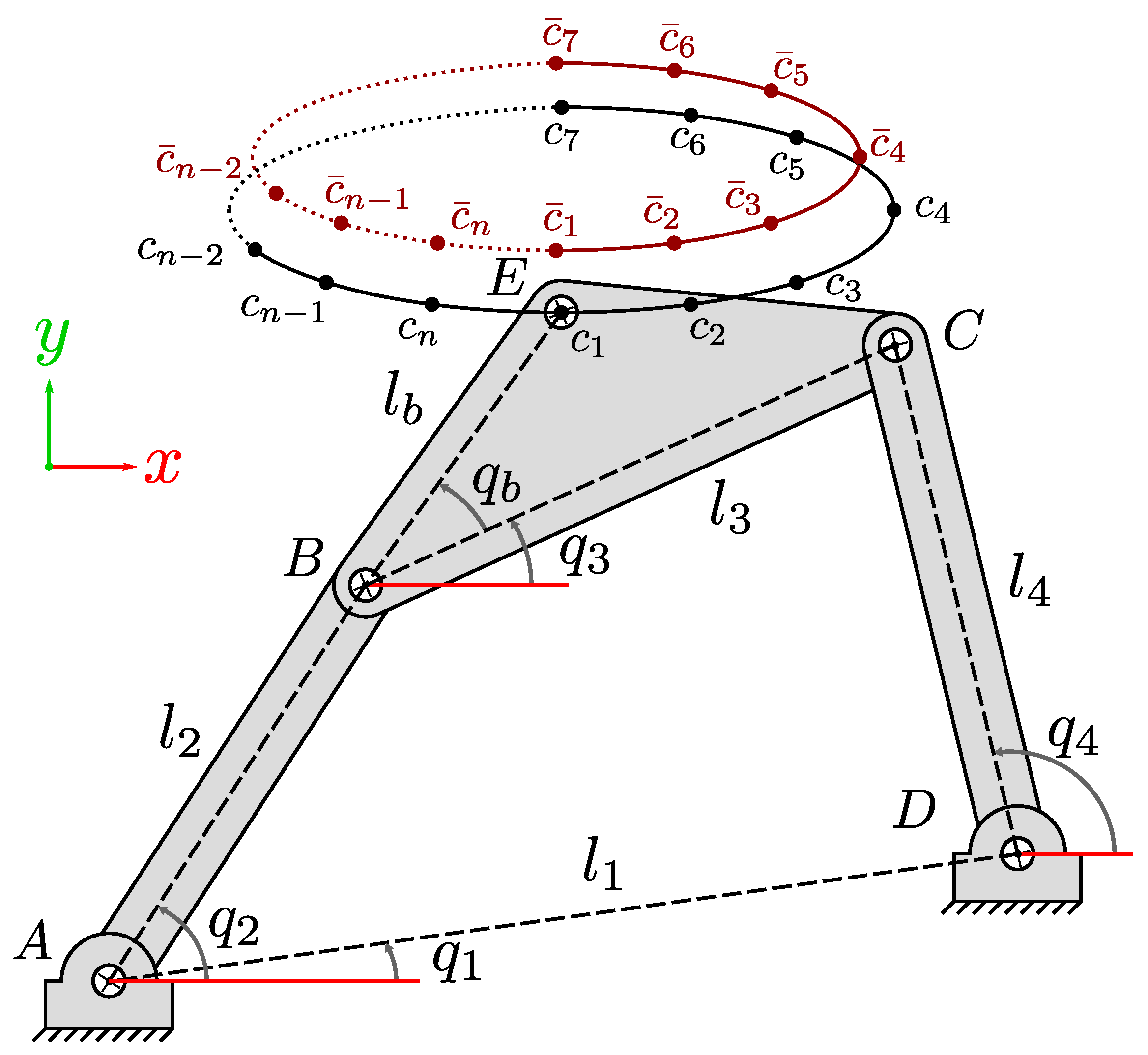
Generally speaking, the four-bar mechanism can be represented in the schematic diagram in Figure 1. In this figure, $l_i$ is the length of the i-th bar, and $q_i$ is its corresponding orientation with respect to the horizontal for all $i=1,2,3,4$. In this representation, the points $A={[x_a,y_a]}^T$ and $D={[x_d,y_d]}^T$ are fixed and are measured with respect to an $XY$ coordinate system. On the other side, the point of interest $E={[x_e,y_e]}^T$ (i.e., the point at which a desired trajectory is developed) in an $XY$ system can be calculated from the point B using the length $l_b$ and the angles $q_3$ (the orientation of the third bar) and $q_b$ (a fixed angle). Moreover, $q_2$ is assumed as the input angle for the mechanism.

To determine the trajectory or path generated by E from the possible values of the input $q_2$, it is necessary to carry out a kinematic study of the mechanism. This study describes the unknown angles $q_3$ and $q_4$ in terms of the known input $q_2$ based on the closed-loop equation presented in Appendix A. With this information, the position of the point E can be calculated. Therefore, by knowing all the angles of the four-bar mechanism in Figure 1, it is possible to determine the position of the point of interest E for any input $q_2$ as follows:

$$\begin{array}{c}\hfill \begin{array}{cc}\hfill x_e& =x_a+l_{2}cos\left(q_2\right)+l_{b}cos(q_3+q_b)\hfill \\ \hfill y_e& =y_a+l_{2}sin\left(q_2\right)+l_{b}sin(q_3+q_b)\hfill \end{array}\end{array}$$

(1)

2.2. Grashof’s Laws for the Four-Bar Mechanism

In order for the input $q_2$ to rotate freely and the mechanism in Figure 1 to generate closed trajectories from the point of interest, the lengths of its bars must satisfy a condition known as Grashof’s law [17]. This law is described below:

$$l_s+l_l\le l_{m_1}+l_{m_2,}$$

(2)

where $l_s$ is the length of the shortest bar, $l_l$ is the length of the longest bar, and $l_{m_1}$ and $l_{m_2}$ are the lengths of the remaining two bars.

If the condition in (2) is satisfied, the shorter bar can rotate freely.

3. The Problem of Synthesis of Four-Bar Grashof-Type Mechanisms

A single-objective mathematical programming problem can be expressed as in (3)–(6). The solution to the above problem is a design vector $\overrightarrow{p}$ with D design variables within the solution space bounded by ${\overrightarrow{p}}_l$ and ${\overrightarrow{p}}_u$ (6) whose variables minimize the value of the objective function $J\left(\overrightarrow{p}\right)$ in (3) (i.e., a quantitative measure that determines the performance of a solution) while satisfying the soft constraints in (4) (i.e., conditions that can be met with a certain degree of slack) and the hard constraints in (5) (i.e., those that must be complied with exactly).

$$\begin{array}{c}\mathbf{min}\\ \overrightarrow{p}\end{array}J\left(\overrightarrow{p}\right)$$

(3)

is subject to

$$g_i\left(\overrightarrow{p}\right)\le 0,i=1,2,\dots ,n_g$$

(4)

$$h_j\left(\overrightarrow{p}\right)=0,j=1,2,\dots ,n_h$$

(5)

$${\overrightarrow{p}}_l\le \overrightarrow{p}\le {\overrightarrow{p}}_u$$

(6)

The dimensional synthesis problem of the four-bar Grashof-type mechanism can be stated in the form of (3)–(6) and can be characterized in two ways as described below.

3.1. The General Problem of Dimensional Synthesis

The general problem for the synthesis of four-bar Grashof-type mechanisms consists of finding the dimensional parameters in $\overrightarrow{p}$ that minimize the differences between the trajectory that the mechanism develops with them and the desired path. Of course, a continuous trajectory is made up of an infinite number of points, and an exact comparison between two of them to determine their differences is unfeasible. In practice, the desired trajectory is described in terms of n representative precision points ${\overline{c}}_i,i=1,2,\dots ,n$, as suggested by the diagram in Figure 1. Thus, the cost function can be written as in (7) to quantify the differences between the n precision points of the desired trajectory and the n points generated by the mechanism with different values of the input $q_2$. In (7), ${\Vert {\overline{c}}_i-c_i\Vert }^2$ is the square norm of the difference between the i-th precision point ${\overline{c}}_i$ from the desired trajectory and $c_i$, which coincides with the point $E={[x_e,y_e]}^T$ of the mechanism when it is subject to the input $q_{2,i}$.

$$J\left(\overrightarrow{p}\right)=\sum _{i=1}^n{\Vert {\overline{c}}_i-c_i\Vert }^2$$

(7)

On the other hand, the lengths of the bars in the four-bar mechanism must satisfy (2) so that at least one of the bars can rotate freely. In this sense, it is aimed that the bar $l_2$ rotates completely with respect to the fixed bar $l_1$, i.e., that the input $q_2$ can take any value to generate closed trajectories with the point E. To guarantee the above, the constraints are set to (8).

$$\begin{array}{c}\hfill \begin{array}{cc}\hfill g_1:& l_1+l_2-l_3-l_4\le 0\hfill \\ \hfill g_2:& l_2+l_4-l_1-l_3\le 0\hfill \\ \hfill g_3:& l_1+l_3-l_1-l_4\le 0\hfill \end{array}\end{array}$$

(8)

Finally, box constraints are used in the dimensional synthesis problem to limit the space occupied by the complete mechanism and to ensure that its manufacture is possible.

On the other side, two conceptualizations of the mechanism synthesis problem can be found in the specialized literature, which are detailed below.

3.2. Synthesis Problem with Prescribed Time

This problem consists of finding the dimensional parameters of the four-bar mechanism when the values of the input $q_2$, which must be used to reach each of the precision points, are known a priori. Thus, for the mechanism in Figure 1, the vector of dimensional variables has the form in (9), and the synthesis problem is subject to the known inputs of the mechanism $q_{2,i},i=1,2,\dots ,n$.

$$\overrightarrow{p}={[x_a,y_a,x_b,y_b,l_1,l_2,l_3,l_4,l_b,q_b]}^T$$

(9)

3.3. Synthesis Problem without Prescribed Time

When the n values of the inputs $q_{2,i},i=1,2,\dots ,n$ required to reach each precision point are unknown, they are included as part of the solution to the synthesis problem, as seen in the vector of design variables in (10).

$$\overrightarrow{p}={[x_a,y_a,x_b,y_b,l_1,l_2,l_3,l_4,l_b,q_b,q_{2,1},q_{2,2},\dots ,q_{2,n}]}^T$$

(10)

4. Differential Evolution

The synthesis problem presented in Section 3 is highly nonlinear and subject to several constraints, and the possible combinations of dimensional parameters are incommensurable. Because of this, the metaheuristic techniques from evolutionary computation and swarm intelligence [36] are alternatives used to obtain adequate solutions to this type of problem at an affordable computational cost [27]. As previously discussed, the metaheuristic technique of Differential Evolution (DE) [30] has been very successful in finding the solutions of dimensional synthesis problems of mechanisms [31,32,33].

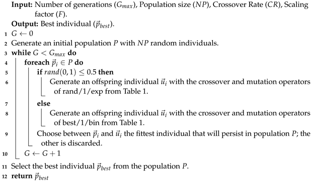
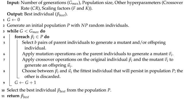
DE is a simple and effective stochastic algorithm for solving challenging optimization problems. This algorithm is inspired by the theory of the natural evolution of species according to Neo-Darwinism. Algorithm 1 summarizes the overall DE operation. At the beginning of the DE (lines 1 and 2), an initial population P is generated with $NP$ random individuals (candidate solutions to an optimization problem randomly generated between bounds ${\overrightarrow{p}}_l$ and ${\overrightarrow{p}}_u$). Subsequently, an evolutionary cycle is executed (lines 3 to 9), and different operations are performed on each individual ${\overrightarrow{p}}_i$ in the population P (lines 4 to 8) to try to improve the original solutions and achieve convergence. Thus, for each ${\overrightarrow{p}}_i$, b pairs of parent individuals are selected (line 5). These generate a ${\overrightarrow{v}}_i$ mutant individual (line 6). Next, the mutant individual ${\overrightarrow{v}}_i$ is recombined with the original ${\overrightarrow{p}}_i$ to obtain an offspring ${\overrightarrow{u}}_i$ (line 7). Finally, the offspring individual ${\overrightarrow{u}}_i$ competes with the original ${\overrightarrow{p}}_i$, and the fittest one persists in population P, while the other is discarded. At the end of the evolutionary cycle, the fittest individuals are expected to be in the population P, from which the best alternative is chosen as the solution to the optimization problem (lines 10 and 11).

Algorithm 1: Differential Evolution

4.1. Differential Evolution Variants

DE has different variants that refer to different ways of performing the mutation and crossover operations in the algorithm 1 (lines 6 and 7). The nomenclature $a/b/c$ is commonly used to denote each variant. In this nomenclature, a refers to the strategy used to compute the mutant individual ${\overrightarrow{v}}_i$, b is the number of pairs of parent individuals used during this computation, and c is the strategy to generate the offspring individual ${\overrightarrow{u}}_i$. Some of the most commonly used variants of DE are described in [37] and are summarized in

Table 1. Some of the most commonly used variants of Differential Evolution.

Nomenclature	Variant
best/b/bin	${\overrightarrow{u}}_{i,j}=\left\{\begin{array}{cc}{\overrightarrow{p}}_{r_{best},j}+F·{\sum }_{k=1}^b\left({\overrightarrow{p}}_{r_2^k,j}-{\overrightarrow{p}}_{r_1^k,j}\right)\hfill & \mathbf{if} rand(0,1)<CR \mathbf{or} j=j_{rand}\hfill \\ {\overrightarrow{p}}_{i,j}\hfill & \mathbf{otherwise}\hfill \end{array}\right.$
best/b/exp	${\overrightarrow{u}}_{i,j}=\left\{\begin{array}{cc}{\overrightarrow{p}}_{r_{best},j}+F·{\sum }_{k=1}^b\left({\overrightarrow{p}}_{r_2^k,j}-{\overrightarrow{p}}_{r_1^k,j}\right)\hfill & \mathbf{from} rand(0,1)<CR \mathbf{or} j=j_{rand}\hfill \\ {\overrightarrow{p}}_{i,j}\hfill & \mathbf{otherwise}\hfill \end{array}\right.$
current-to-best/b	${\overrightarrow{u}}_i={\overrightarrow{p}}_i+K·\left({\overrightarrow{p}}_{r_{best}}-{\overrightarrow{p}}_i\right)+F·{\sum }_{k=1}^b\left({\overrightarrow{p}}_{r_2^k}-{\overrightarrow{p}}_{r_1^k}\right)$
current-to-rand/b	${\overrightarrow{u}}_i={\overrightarrow{p}}_i+K·\left({\overrightarrow{p}}_{r_3}-{\overrightarrow{p}}_i\right)+F·{\sum }_{k=1}^b\left({\overrightarrow{p}}_{r_2^k}-{\overrightarrow{p}}_{r_1^k}\right)$
current-to-rand/b/bin	${\overrightarrow{u}}_{i,j}=\left\{\begin{array}{cc}{\overrightarrow{p}}_{i,j}+K·\left({\overrightarrow{p}}_{r_3,j}-{\overrightarrow{p}}_{i,j}\right)+F·{\sum }_{k=1}^b\left({\overrightarrow{p}}_{r_2^k,j}-{\overrightarrow{p}}_{r_1^k,j}\right)\hfill & \mathbf{if} rand(0,1)<CR \mathbf{or} j=j_{rand}\hfill \\ {\overrightarrow{p}}_{i,j}\hfill & \mathbf{otherwise}\hfill \end{array}\right.$
rand/b/bin	${\overrightarrow{u}}_{i,j}=\left\{\begin{array}{cc}{\overrightarrow{p}}_{r_3,j}+F·{\sum }_{k=1}^b\left({\overrightarrow{p}}_{r_2^k,j}-{\overrightarrow{p}}_{r_1^k,j}\right)\hfill & \mathbf{if} rand(0,1)<CR \mathbf{or} j=j_{rand}\hfill \\ {\overrightarrow{p}}_{i,j}\hfill & \mathbf{otherwise}\hfill \end{array}\right.$
rand/b/exp	${\overrightarrow{u}}_{i,j}=\left\{\begin{array}{cc}{\overrightarrow{p}}_{r_3,j}+F·{\sum }_{k=1}^b\left({\overrightarrow{p}}_{r_2^k,j}-{\overrightarrow{p}}_{r_1^k,j}\right)\hfill & \mathbf{from} rand(0,1)<CR \mathbf{or} j=j_{rand}\hfill \\ {\overrightarrow{p}}_{i,j}\hfill & \mathbf{otherwise}\hfill \end{array}\right.$
rand/2/dir	${\overrightarrow{u}}_i=\begin{array}{cc}{\overrightarrow{p}}_{r_1}+\frac{F}{2}·\left({\overrightarrow{p}}_{r_1}-{\overrightarrow{p}}_{r_2}+{\overrightarrow{p}}_{r_3}-{\overrightarrow{p}}_{r_4}\right)\hfill & \mathbf{where} fit\left({\overrightarrow{p}}_{r_1}\right)>fit\left({\overrightarrow{p}}_{r_2}\right) \mathbf{and} fit\left({\overrightarrow{p}}_{r_3}\right)>fit\left({\overrightarrow{p}}_{r_4}\right)\hfill \end{array}$

. In this table, $rand(0,1)$ is a random number generated from a uniform probability distribution in the interval [0, 1], j is the j-th design variable of an individual, and $j_{rand}$ is a randomly selected design variable. On the other hand, ${\overrightarrow{p}}_{r_3}$, ${\overrightarrow{p}}_{r_2^k}$, and ${\overrightarrow{p}}_{r_1^k}$ for the first seven variants, are individuals randomly selected from the population P, such that $i\ne r_3\ne r_2^k\ne r_1^k$, with k as the number of parent pairs, while ${\overrightarrow{p}}_{r_{best}}$ is the fittest solution in P. For the variant rand/2/dir, ${\overrightarrow{p}}_{r_1}$, ${\overrightarrow{p}}_{r_2}$, ${\overrightarrow{p}}_{r_3}$, and ${\overrightarrow{p}}_{r_4}$ are individuals randomly selected from P such that $i\ne r_1\ne r_2\ne r_3\ne r_4$, and they also satisfy $fit\left({\overrightarrow{p}}_{r_1}\right)>fit\left({\overrightarrow{p}}_{r_2}\right)$ and $fit\left({\overrightarrow{p}}_{r_3}\right)>fit\left({\overrightarrow{p}}_{r_4}\right)$. Ultimately, $CR\in$ [0, 1] is the crossover rate, and $F,K\in$ [0, 1] are scaling factors, which are all DE hyperparameters.

Each DE variant intends to improve its ability to perform exploratory searches (i.e., to find promising regions of the search space), exploitative searches (i.e., to find good solutions in particular regions of the search space), or to maintain an appropriate balance between the two.

4.2. Simple and Improved Differential Evolution

Advancing the results of Section 5, a Simple and Improved DE (SIDE) is now presented. The SIDE combines the behavior of the two most prominent variants of DE to solve the mechanism synthesis problem. These variants are rand/1/exp and best/1/bin. On the one hand, rand/1/exp has a great exploratory capacity that allows for finding different syntheses of mechanisms to follow a trajectory conformed by precision points. On the other hand, best/1/bin has a higher exploitative ability to refine the performance of a particular synthesis of the mechanism. In this way, SIDE takes advantage of the exploratory capacity of rand/1/exp and the exploitative ability of best/1/bin. The operation of SIDE is presented in Algorithm 2. Unlike the general functionality of the DE variants, described by Algorithm 1, in each generation G (line 3) and for each individual ${\overrightarrow{p}}_i$ in the current population (line 4), SIDE decides randomly and with equal probability (line 5) which crossover and mutation operations to perform between those of rand/1/exp (line 6) and best/1/bin (line 8). This keeps the balance between exploration and exploitation simple.

4.3. Measuring the Fitness of Individuals

When an optimization problem includes neither equality nor inequality constraints, each individual’s fitness in the DE can be measured in terms of the value of the objective function. For minimization, the smaller the value of the objective function evaluated on an individual, the fitter the individual is. At the other extreme, where the optimization problem is subject to such constraints, the fitness must also consider the fulfillment of the constraints. One of the simplest and most efficient methods for comparing the fitness of two different solutions in terms of feasibility (compliance with equality and inequality constraints) and optimality (minimization of the objective function) is known as Deb’s rules [38]. For two distinct solutions ${\overrightarrow{p}}_1$ and ${\overrightarrow{p}}_2$, these rules state the following:

• If ${\overrightarrow{p}}_1$ is feasible and ${\overrightarrow{p}}_2$ is unfeasible, then ${\overrightarrow{p}}_1$ is fitter, i.e., $fit\left({\overrightarrow{p}}_1\right)>fit\left({\overrightarrow{p}}_2\right)$. When the contrary occurs, i.e., ${\overrightarrow{p}}_1$ is unfeasible and ${\overrightarrow{p}}_2$ is feasible, then $fit\left({\overrightarrow{p}}_1\right)<fit\left({\overrightarrow{p}}_2\right)$;
• If both ${\overrightarrow{p}}_1$ and ${\overrightarrow{p}}_2$ are feasible, the solution with the smaller objective function value is fitter (for minimization problems);
• If both ${\overrightarrow{p}}_1$ and ${\overrightarrow{p}}_2$ are unfeasible, the solution with the smaller value of the constraint violation sum is fitter.

Algorithm 2: SIDE: Simple and Improved Differential Evolution (based on the DE variants rand/1/exp and best/1/bin

The constraint violation sum for a candidate solution $\overrightarrow{p}$ of any constrained optimization problem can be calculated as follows:

$$\varphi \left(\overrightarrow{p}\right)=\sum _{i=1}^{n_g}\max {\left\{0,g_i\left(\overrightarrow{p}\right)\right\}}^2+\sum _{j=1}^{n_h}\left|h_j\left(\overrightarrow{p}\right)\right|$$

(11)

The rules described in this section are used in DE when it is necessary to choose the fittest solution (Algorithm 1 lines 8 and 10) or when some variant requires discriminating solutions to establish a suitable search direction in mutation or crossover operations (variant rand/2/dir in Table 1).

4.4. Complexity of Differential Evolution

As described in [39], the DE variants perform an evolutionary cycle of $G_{max}$ generations to apply mutation and recombination operations on the D design variables of each of the $NP$ individuals in the population. Thus, the execution time of this algorithm is proportional to the three variables above. Therefore, the computational complexity of DE and its variants, including SIDE, can be expressed in the Big O notation as

$$O\left(D·NP·G_{max}\right)$$

(12)

5. Results and Discussion

5.1. Experiment Details

The case studies for the comparative analysis were taken from the benchmark gathered in [40]. This benchmark includes four case studies:

• Case C1: It includes six precision points and has no prescribed time.
• Case C2: As in C1, six accuracy points are specified, but this time, the prescribed time is considered.
• Case C3: This case has ten precision points with no prescribed time.
• Case C4: This case contains eighteen precision points and a prescribed time. In this particular case, the vector of design variables (9) additionally includes $q_{2,0}$, i.e., an initial angle for the prescribed time calculation.

The precision points for each case study and the prescribed time are given in

Table 2. Benchmark case studies gathered in [40].

Case Study	Precision Points (mm)	PRESCRIBED Time (Rad)
C1	${\overline{c}}_1={[20,20]}^T$, ${\overline{c}}_2={[20,25]}^T$, ${\overline{c}}_3={[20,30]}^T$, ${\overline{c}}_4={[20,35]}^T$, ${\overline{c}}_5={[20,40]}^T$, ${\overline{c}}_6={[20,45]}^T$	−
C2	${\overline{c}}_1={[0,0]}^T$, ${\overline{c}}_2={[1.9098,5.8779]}^T$, ${\overline{c}}_3={[6.9098,9.5106]}^T$, ${\overline{c}}_4={[13.09,9.5106]}^T$, ${\overline{c}}_5={[18.09,5.8779]}^T$, ${\overline{c}}_6={[20,0]}^T$	$q_{2,1}=\frac{\pi }{6}$, $q_{2,2}=\frac{\pi }{3}$, $q_{2,3}=\frac{\pi }{2}$, $q_{2,4}=\frac{2\pi }{3}$, $q_{2,5}=\frac{5\pi }{6}$, $q_{2,6}=\pi$
C3	${\overline{c}}_1={[20,10]}^T$, ${\overline{c}}_2={[17.66,15.142]}^T$, ${\overline{c}}_3={[11.736,17.878]}^T$, ${\overline{c}}_4={[5,16.928]}^T$, ${\overline{c}}_5={[0.60307,12.736]}^T$, ${\overline{c}}_6={[0.60307,7.2638]}^T$, ${\overline{c}}_7={[5,3.0718]}^T$, ${\overline{c}}_8={[11.736,2.1215]}^T$, ${\overline{c}}_9={[17.66,4.8577]}^T$, ${\overline{c}}_{10}={[20,10]}^T$	−
C4	${\overline{c}}_1={[0.5,1.1]}^T$, ${\overline{c}}_2={[0.4,1.1]}^T$, ${\overline{c}}_3={[0.3,1.1]}^T$, ${\overline{c}}_4={[0.2,1.0]}^T$, ${\overline{c}}_5={[0.1,0.9]}^T$, ${\overline{c}}_6={[0.005,0.75]}^T$, ${\overline{c}}_7={[0.02,0.6]}^T$, ${\overline{c}}_8={[0.0,0.5]}^T$, ${\overline{c}}_9={[0.0,0.4]}^T$, ${\overline{c}}_{10}={[0.03,0.3]}^T$, ${\overline{c}}_{11}={[0.1,0.25]}^T$, ${\overline{c}}_{12}={[0.15,0.2]}^T$, ${\overline{c}}_{13}={[0.2,0.3]}^T$, ${\overline{c}}_{14}={[0.3,0.4]}^T$, ${\overline{c}}_{15}={[0.4,0.5]}^T$, ${\overline{c}}_{16}={[0.5,0.7]}^T$, ${\overline{c}}_{17}={[0.6,0.9]}^T$, ${\overline{c}}_{18}={[0.6,1.0]}^T$	$q_{2,i}=q_{2,0}+\frac{2\pi }{18}i,i=1,2,\dots ,18$

.

For the dimensional synthesis problem associated with each case study, the search space was delimited according to the bounds of the design variables, as shown in

Table 3. Bounds of the search space for the benchmark case studies gathered in [40].

Variable	Case 1		Case 2		Case 3		Case 4
${\overrightarrow{\mathit{p}}}_{\mathit{j}}$	${\overrightarrow{\mathit{p}}}_{\mathit{l},\mathit{j}}$	${\overrightarrow{\mathit{p}}}_{\mathit{u},\mathit{j}}$	${\overrightarrow{\mathit{p}}}_{\mathit{l},\mathit{j}}$	${\overrightarrow{\mathit{p}}}_{\mathit{u},\mathit{j}}$	${\overrightarrow{\mathit{p}}}_{\mathit{l},\mathit{j}}$	${\overrightarrow{\mathit{p}}}_{\mathit{u},\mathit{j}}$	${\overrightarrow{\mathit{p}}}_{\mathit{l},\mathit{j}}$	${\overrightarrow{\mathit{p}}}_{\mathit{u},\mathit{j}}$
$x_a$ ($\mathrm{mm}$)	−60	60	−50	50	−80	80	−50	50
$y_a$ ($\mathrm{mm}$)	−60	60	−50	50	−80	80	−50	50
$x_d$ ($\mathrm{mm}$)	−60	60	−50	50	−80	80	−50	50
$y_d$ ($\mathrm{mm}$)	−60	60	−50	50	−80	80	−50	50
$l_2$ ($\mathrm{mm}$)	5	60	5	50	5	80	0	50
$l_3$ ($\mathrm{mm}$)	5	60	5	50	5	80	0	50
$l_4$ ($\mathrm{mm}$)	5	60	5	50	5	80	0	50
$l_b$ ($\mathrm{mm}$)	5	60	5	50	5	80	0	50
$q_b$ ($\mathrm{rad}$)	0	2$\pi$	0	2$\pi$	0	2$\pi$	0	2$\pi$
$q_{2,0}$ ($\mathrm{rad}$)	−	−	−	−	−	−	0	2$\pi$
$q_{2,i}$ ($\mathrm{rad}$)	0	2$\pi$	−	−	0	2$\pi$	−	−

Note: j refers to the j-th design variable of a solution.

.

On the other hand, the DE variants used in the comparative analysis included the eight studied in [37], i.e., best/1/bin, best/1/exp, current-to-best/1, current-to-rand/1, current-to-rand/1/bin, rand/1/bin, rand/1/exp, and rand/2/dir. For each variant, the population size $NP=100$ and a maximum number of generations $G_{max}$ = 10,000 were set to provide the DE with sufficient evaluations of the optimization problem to complete the synthesis of the mechanisms. Concerning the hyperparameters used in the DE variants, a fixed value was chosen for the crossover probability $CR=0.5$, and the scaling factors F and K were calculated randomly at the beginning of each generation in the interval $[0.3,0.9]$ as suggested in [37].

5.2. Analysis of Results among DE Variants

In order to carry out the comparative study, 30 independent runs of each DE variant were performed on each of the previously described case studies. The above process was performed to collect enough information to describe the behavior of each variant. Each of the executions was performed in a PC with Intel(R) Core(TM) i9-10900K CPU @ 3.70 GHz and 32 GB of RAM. The algorithms were written in C++ programs.

Table 4. Descriptive results for case study C1 concerning the value of the objective function $J\left(\overrightarrow{p}\right)$.

Variant	Min $\mathit{J}\left(\overrightarrow{\mathit{p}}\right)$	Max $\mathit{J}\left(\overrightarrow{\mathit{p}}\right)$	Mean $\mathit{J}\left(\overrightarrow{\mathit{p}}\right)$	Std $\mathit{J}\left(\overrightarrow{\mathit{p}}\right)$
rand/1/bin	3.2919 $\times {10}^{-2}$	2.2387 $\times {10}^1$	1.0145	4.0762
rand/1/exp	4.7963 $\times {10}^{-28}$	1.5917 $\times {10}^{-2}$	1.3047 $\times {10}^{-3}$	3.3223 $\times {10}^{-3}$
best/1/bin	4.9180 $\times {10}^{-4}$	1.2401	1.2289 $\times {10}^{-1}$	2.5584 $\times {10}^{-1}$
best/1/exp	9.1777 $\times {10}^{-5}$	3.4345	1.5169 $\times {10}^{-1}$	6.2857 $\times {10}^{-1}$
current-to-rand/1	2.6946 $\times {10}^{-2}$	1.5198 $\times {10}^1$	3.5729	4.2861
current-to-best/1	1.6866 $\times {10}^{-2}$	6.2969 $\times {10}^1$	1.1066 $\times {10}^1$	1.4955 $\times {10}^1$
current-to-rand/1/bin	5.6907 $\times {10}^{-2}$	6.9120	2.7548	1.6211
rand/2/dir	2.1001 $\times {10}^{-1}$	4.2374 $\times {10}^1$	1.2032 $\times {10}^1$	1.2016 $\times {10}^1$

,

Table 5. Descriptive results for case study C2 concerning the value of the objective function $J\left(\overrightarrow{p}\right)$.

Variant	Min $\mathit{J}\left(\overrightarrow{\mathit{p}}\right)$	Max $\mathit{J}\left(\overrightarrow{\mathit{p}}\right)$	Mean $\mathit{J}\left(\overrightarrow{\mathit{p}}\right)$	Std $\mathit{J}\left(\overrightarrow{\mathit{p}}\right)$
rand/1/bin	7.8661 $\times {10}^{-1}$	1.5482 $\times {10}^1$	3.7318	5.9757
rand/1/exp	7.8637 $\times {10}^{-1}$	1.5482 $\times {10}^1$	8.1343	7.4736
best/1/bin	7.8637 $\times {10}^{-1}$	1.5482 $\times {10}^1$	9.1141	7.4069
best/1/exp	7.8637 $\times {10}^{-1}$	1.7626 $\times {10}^1$	7.9973	7.7361
current-to-rand/1	7.8637 $\times {10}^{-1}$	2.2261 $\times {10}^1$	5.7107	7.9301
current-to-best/1	8.0896 $\times {10}^{-1}$	2.6194 $\times {10}^1$	9.7399	8.5027
current-to-rand/1/bin	7.8637 $\times {10}^{-1}$	8.1010	1.4586	1.8089
rand/2/dir	7.8637 $\times {10}^{-1}$	1.5557 $\times {10}^1$	6.6826	7.3202

,

Table 6. Descriptive results for case study C3 concerning the value of the objective function $J\left(\overrightarrow{p}\right)$.

Variant	Min $\mathit{J}\left(\overrightarrow{\mathit{p}}\right)$	Max $\mathit{J}\left(\overrightarrow{\mathit{p}}\right)$	Mean $\mathit{J}\left(\overrightarrow{\mathit{p}}\right)$	Std $\mathit{J}\left(\overrightarrow{\mathit{p}}\right)$
rand/1/bin	8.9514 $\times {10}^{-2}$	4.8844 $\times {10}^{-1}$	2.0483 $\times {10}^{-1}$	1.1031 $\times {10}^{-1}$
rand/1/exp	1.4882 $\times {10}^{-4}$	8.6580 $\times {10}^{-4}$	3.5663 $\times {10}^{-4}$	2.2381 $\times {10}^{-4}$
best/1/bin	1.7205 $\times {10}^{-4}$	2.4649	2.2577 $\times {10}^{-1}$	6.3549 $\times {10}^{-1}$
best/1/exp	3.5591 $\times {10}^{-1}$	3.0170 $\times {10}^2$	7.6570 $\times {10}^1$	8.7209 $\times {10}^1$
current-to-rand/1	3.2355 $\times {10}^{-1}$	1.3797 $\times {10}^2$	2.2160 $\times {10}^1$	3.0723 $\times {10}^1$
current-to-best/1	1.5225	3.3413 $\times {10}^2$	9.9118 $\times {10}^1$	1.0246 $\times {10}^2$
current-to-rand/1/bin	3.2461 $\times {10}^{-2}$	2.5930	6.5177 $\times {10}^{-1}$	6.2819 $\times {10}^{-1}$
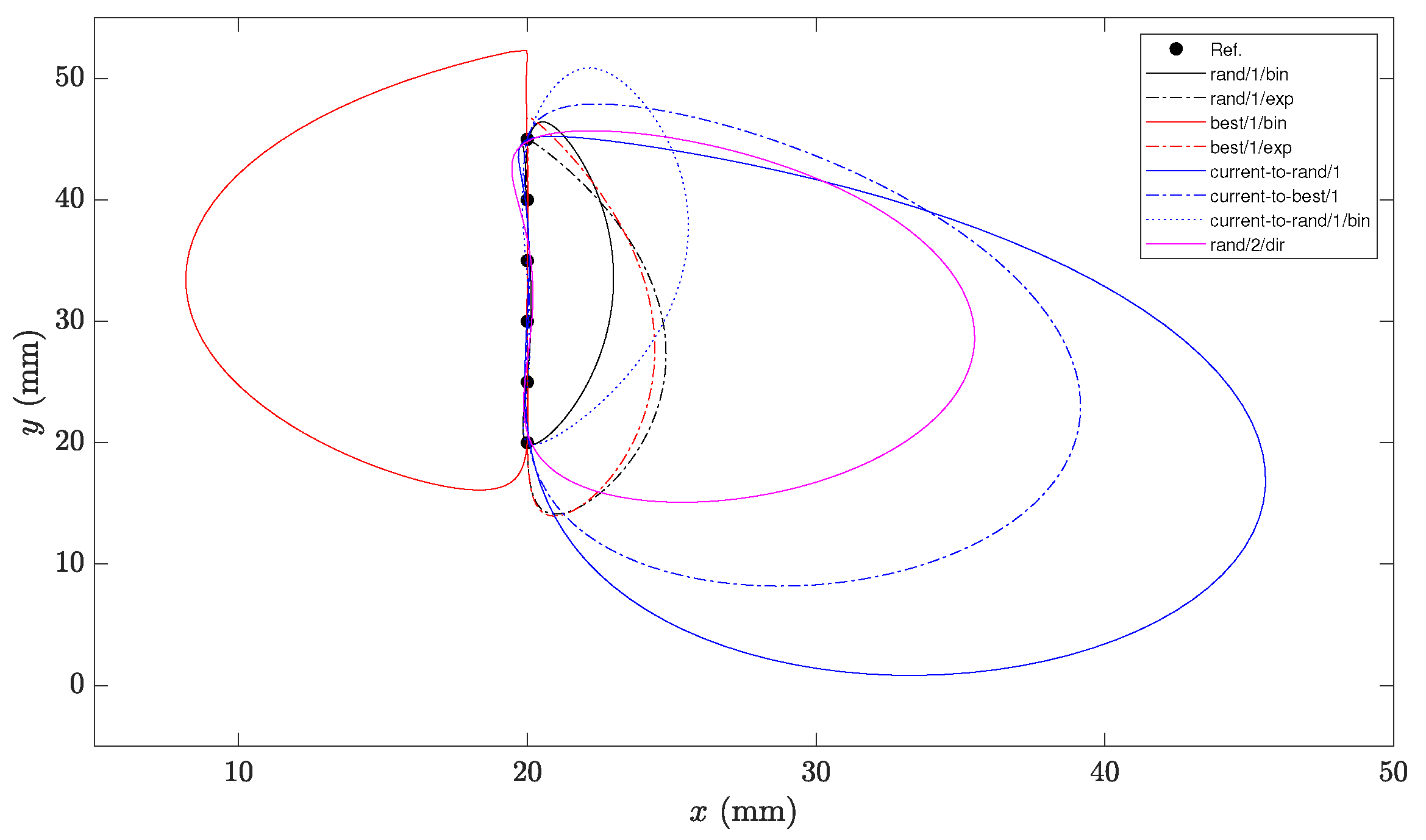
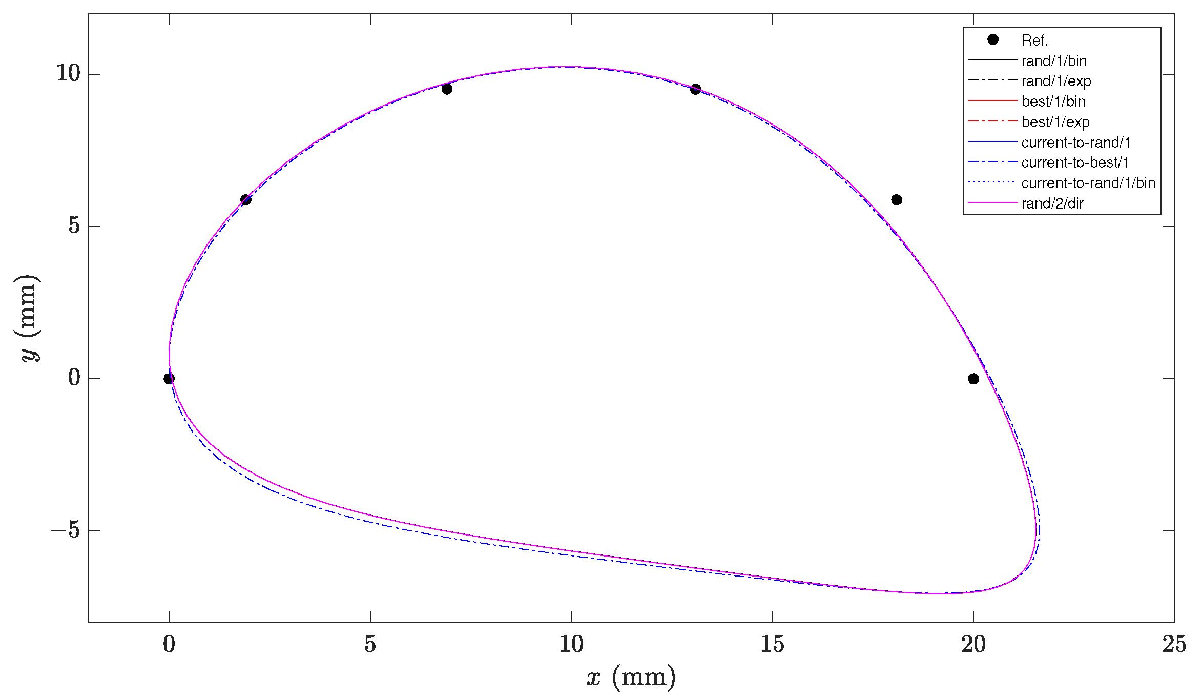
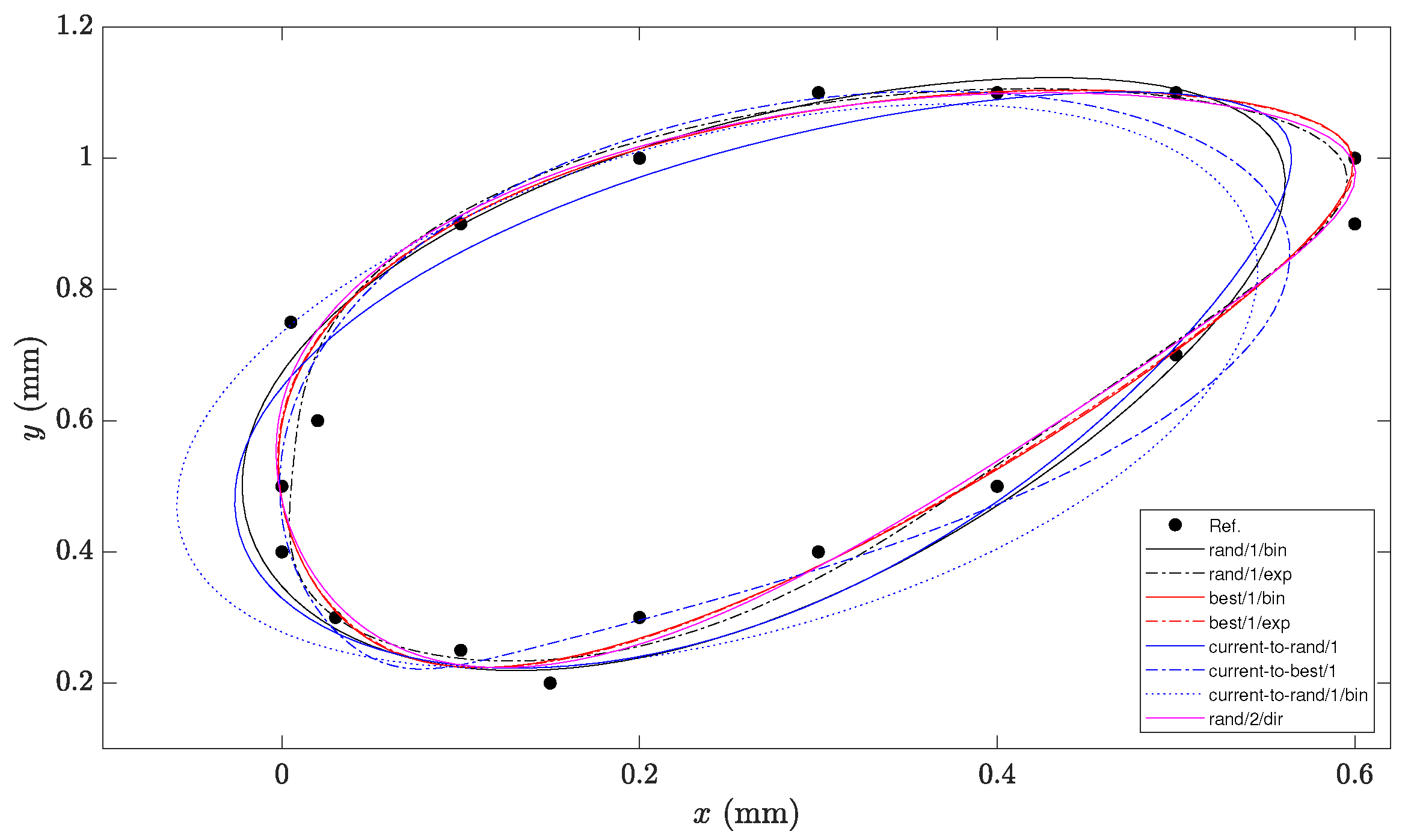
rand/2/dir	8.7032	2.0594 $\times {10}^2$	7.5678 $\times {10}^1$	5.3282 $\times {10}^1$

and

Table 7. Descriptive results for case study C4 concerning the value of the objective function $J\left(\overrightarrow{p}\right)$.

Variant	Min $\mathit{J}\left(\overrightarrow{\mathit{p}}\right)$	Max $\mathit{J}\left(\overrightarrow{\mathit{p}}\right)$	Mean $\mathit{J}\left(\overrightarrow{\mathit{p}}\right)$	Std $\mathit{J}\left(\overrightarrow{\mathit{p}}\right)$
rand/1/bin	2.6384 $\times {10}^{-2}$	1.6941 $\times {10}^{-1}$	9.9931 $\times {10}^{-2}$	4.0570 $\times {10}^{-2}$
rand/1/exp	9.9119 $\times {10}^{-3}$	3.9021 $\times {10}^{-2}$	1.9031 $\times {10}^{-2}$	1.0140 $\times {10}^{-2}$
best/1/bin	1.0859 $\times {10}^{-2}$	4.6205 $\times {10}^{-2}$	3.0999 $\times {10}^{-2}$	1.2643 $\times {10}^{-2}$
best/1/exp	1.0729 $\times {10}^{-2}$	2.5308	6.4464 $\times {10}^{-1}$	1.0652
current-to-rand/1	2.2665 $\times {10}^{-2}$	2.6011 $\times {10}^{-1}$	5.1780 $\times {10}^{-2}$	4.3035 $\times {10}^{-2}$
current-to-best/1	3.3125 $\times {10}^{-2}$	2.5308	8.5767 $\times {10}^{-1}$	1.1200
current-to-rand/1/bin	7.0545 $\times {10}^{-2}$	1.5315 $\times {10}^{-1}$	1.1459 $\times {10}^{-1}$	1.9138 $\times {10}^{-2}$
rand/2/dir	1.0672 $\times {10}^{-2}$	4.5639 $\times {10}^{-2}$	2.7762 $\times {10}^{-2}$	1.1192 $\times {10}^{-2}$

present the statistical results of the experiments performed concerning the value of the objective function $J\left(\overrightarrow{p}\right)$. Moreover, the statistics on the execution time t of all variants are summarized in

Table 8. Descriptive results for case study C1 concerning the execution time t.

Variant	Min t (s)	Max t (s)	Mean t (s)	Std t (s)
rand/1/bin	1.9860	2.3810	2.0911	7.6625 $\times {10}^{-2}$
rand/1/exp	1.9580	2.4860	2.2930	1.4654 $\times {10}^{-1}$
best/1/bin	1.9040	2.9310	2.4808	3.1398 $\times {10}^{-1}$
best/1/exp	2.1200	2.7530	2.4680	2.0237 $\times {10}^{-1}$
current-to-rand/1	2.2250	2.3070	2.2728	2.0898 $\times {10}^{-2}$
current-to-best/1	1.2250	2.5610	2.4084	3.1461 $\times {10}^{-1}$
current-to-rand/1/bin	2.0810	2.3380	2.2274	6.0469 $\times {10}^{-2}$
rand/2/dir	1.8990	2.3310	2.2566	9.3149 $\times {10}^{-2}$

,

Table 9. Descriptive results for case study C2 concerning the execution time t.

Variant	Min t (s)	Max t (s)	Mean t (s)	Std t (s)
rand/1/bin	1.7490	2.1290	2.0658	6.6250 $\times {10}^{-2}$
rand/1/exp	2.0840	2.1770	2.1334	3.1339 $\times {10}^{-2}$
best/1/bin	2.6380	2.8540	2.7955	4.2712 $\times {10}^{-2}$
best/1/exp	2.3830	2.4660	2.4214	2.9671 $\times {10}^{-2}$
current-to-rand/1	1.9430	2.0900	2.0276	3.9621 $\times {10}^{-2}$
current-to-best/1	2.0050	2.3340	2.2448	6.9939 $\times {10}^{-2}$
current-to-rand/1/bin	1.5270	2.0720	1.8059	1.7287 $\times {10}^{-1}$
rand/2/dir	1.8820	2.1040	2.0429	5.7365 $\times {10}^{-2}$

,

Table 10. Descriptive results for case study C3 concerning the execution time t.

Variant	Min t (s)	Max t (s)	Mean t (s)	Std t (s)
rand/1/bin	3.2880	3.5230	3.4037	5.4166 $\times {10}^{-2}$
rand/1/exp	3.5480	3.6490	3.6162	2.8255 $\times {10}^{-2}$
best/1/bin	3.5060	3.8940	3.7965	1.0321 $\times {10}^{-1}$
best/1/exp	2.8110	3.9540	3.2564	3.5805 $\times {10}^{-1}$
current-to-rand/1	3.2950	3.4290	3.3674	3.2500 $\times {10}^{-2}$
current-to-best/1	3.5020	3.6970	3.6184	5.0301 $\times {10}^{-2}$
current-to-rand/1/bin	3.3810	3.6050	3.4849	5.8481 $\times {10}^{-2}$
rand/2/dir	3.3790	3.4590	3.4094	2.0647 $\times {10}^{-2}$

and

Table 11. Descriptive results for case study C4 concerning the execution time t.

Variant	Min t (s)	Max t (s)	Mean t (s)	Std t (s)
rand/1/bin	2.4970	4.3940	3.4077	4.1057 $\times {10}^{-1}$
rand/1/exp	4.5200	5.1780	4.8404	1.9767 $\times {10}^{-1}$
best/1/bin	3.5810	5.5190	4.6860	6.3739 $\times {10}^{-1}$
best/1/exp	5.1020	5.5660	5.4437	1.1601 $\times {10}^{-1}$
current-to-rand/1	4.7700	5.1690	5.0107	9.7751 $\times {10}^{-2}$
current-to-best/1	4.9310	5.4280	5.2747	1.0424 $\times {10}^{-1}$
current-to-rand/1/bin	4.6220	4.9890	4.8403	9.0887 $\times {10}^{-2}$
rand/2/dir	4.7210	5.2210	5.0707	1.0618 $\times {10}^{-1}$

. The columns of these tables include, in addition to the name of the DE variant, the minimum, maximum, mean, and standard deviation of the objective function $J\left(\overrightarrow{p}\right)$ and the execution time t, respectively, for the 30 independent runs. Moreover, the behavior of the best solutions to the dimensional synthesis problems obtained with each DE variant is shown in Figure 2, Figure 3, Figure 4 and Figure 5 for each case study. The minimum and maximum tracking error e (i.e., the maximum and minimum distances between the precision points and the points generated with the mechanism) for those figures are reported in

Table 12. Minimum and maximum errors e obtained with the best mechanism synthesized by each DE variant for all case studies.

Case Study	Variant	Min e (mm)	Max e (mm)
C1	rand/1/bin	1.5791 $\times {10}^{-2}$	1.2610 $\times {10}^{-1}$
	rand/1/exp	1.9585 $\times {10}^{-4}$	5.5990 $\times {10}^{-4}$
	best/1/bin	1.0844 $\times {10}^{-3}$	1.3547 $\times {10}^{-2}$
	best/1/exp	6.0853 $\times {10}^{-4}$	7.3483 $\times {10}^{-3}$
	current-to-rand/1	2.0705 $\times {10}^{-2}$	9.0178 $\times {10}^{-2}$
	current-to-best/1	1.5673 $\times {10}^{-2}$	7.1780 $\times {10}^{-2}$
	current-to-rand/1/bin	1.5285 $\times {10}^{-2}$	1.7790 $\times {10}^{-1}$
	rand/2/dir	9.4962 $\times {10}^{-2}$	3.4111 $\times {10}^{-1}$
C2	rand/1/bin	7.9554 $\times {10}^{-2}$	6.1321 $\times {10}^{-1}$
	rand/1/exp	7.9865 $\times {10}^{-2}$	6.1541 $\times {10}^{-1}$
	best/1/bin	7.9865 $\times {10}^{-2}$	6.1541 $\times {10}^{-1}$
	best/1/exp	7.9865 $\times {10}^{-2}$	6.1541 $\times {10}^{-1}$
	current-to-rand/1	7.9714 $\times {10}^{-2}$	6.1540 $\times {10}^{-1}$
	current-to-best/1	3.1867 $\times {10}^{-2}$	6.5551 $\times {10}^{-1}$
	current-to-rand/1/bin	7.9873 $\times {10}^{-2}$	6.1545 $\times {10}^{-1}$
	rand/2/dir	7.9215 $\times {10}^{-2}$	6.1579 $\times {10}^{-1}$
C3	rand/1/bin	4.3437 $\times {10}^{-2}$	1.8433 $\times {10}^{-1}$
	rand/1/exp	1.3298 $\times {10}^{-4}$	6.6972 $\times {10}^{-3}$
	best/1/bin	3.1495 $\times {10}^{-4}$	8.3755 $\times {10}^{-3}$
	best/1/exp	5.7835 $\times {10}^{-2}$	2.9000 $\times {10}^{-1}$
	current-to-rand/1	3.3445 $\times {10}^{-2}$	3.7868 $\times {10}^{-1}$
	current-to-best/1	1.4906 $\times {10}^{-1}$	6.3833 $\times {10}^{-1}$
	current-to-rand/1/bin	1.7922 $\times {10}^{-2}$	8.9935 $\times {10}^{-2}$
	rand/2/dir	1.6952 $\times {10}^{-1}$	1.5012
C4	rand/1/bin	1.1348 $\times {10}^{-1}$	3.6744 $\times {10}^{-1}$
	rand/1/exp	1.8390 $\times {10}^{-1}$	6.5760 $\times {10}^{-1}$
	best/1/bin	1.1160 $\times {10}^{-1}$	3.3195 $\times {10}^{-1}$
	best/1/exp	1.8682 $\times {10}^{-1}$	6.9113 $\times {10}^{-1}$
	current-to-rand/1	1.5557 $\times {10}^{-1}$	4.9885 $\times {10}^{-1}$
	current-to-best/1	1.7808 $\times {10}^{-1}$	6.3160 $\times {10}^{-1}$
	current-to-rand/1/bin	1.3716 $\times {10}^{-1}$	4.0078 $\times {10}^{-1}$
	rand/2/dir	1.8489 $\times {10}^{-1}$	6.9293 $\times {10}^{-1}$

. In all tables, the values in gray background color denote the best results.

Based on the above results, the main findings can be stated as follows:

• In synthesis problems without prescribed timing related to the cases C1 and C3, the results shown in Table 4 and Table 6 indicate that the variant rand/1/exp obtained unbeatable results based on the minimum value achieved in all descriptive indicators when compared to the rest of the variants. Its performance was significantly better than most of the DE variants based on the standard deviation and the search for the best solution. Only the variant best/1/bin performed competitively in the search for the minimum value.
• In synthesis problems with prescribed timing related to the cases C2 and C4, the results shown in Table 5 and Table 7 reveal that the variants current-to-rand/1/bin and rand/1/exp had the best performance in the case C2 and the case C4, respectively, based on the standard deviation and the search for the best solution. In the case C2, all variants, except for rand/1/bin and current-to-best/1, had similar performance results (i.e., they performed competitively) in terms of the minimum value of the objective function $J\left(\overrightarrow{p}\right)$. On the other hand, the variants best/1/bin, best/1/exp, and rand/2/dir performed comparably to rand/1/exp when considering the minimum value of the objective function $J\left(\overrightarrow{p}\right)$ in the case C4. This indicates that the second best promising algorithms in this kind of problem were the variants best/1/bin, best/1/exp, and rand/2/dir. This may be due to the exploratory capacity of these variants.
• Based on the statistical information of the four case studies included in Table 4, Table 5, Table 6 and Table 7, the DE variant rand/1/exp can be considered as the best alternative to solve the problem of synthesizing four-bar Grashof-type mechanisms. Since four-bar mechanisms with different syntheses can produce very similar trajectories [41], the success of the DE variant rand/1/exp may have been attributed in part to the known exploratory ability of the rand variants [42], which made it possible to explore different promising regions of the solution space (i.e., different ways of synthesizing the mechanism). In addition, the use of the exponential recombination exp in rand/1/exp may have increased its performance with respect to problems with a larger number of design variables [43], as in cases C1 and C3, where, in addition to the parameters for the synthesis of the mechanism, the input values that allowed for reaching each precision point were also searched. Here, it is worth noting that, in several of the applications requiring the dimensional synthesis of mechanisms, there is no prescribed time [44,45,46]. This may be caused by the fact that designs are generally aimed to meet in the best possible way some performance criteria, such as accuracy in developing a specific trajectory without limiting the possible solutions. At the same time, the use of prescribed time restricts the alternatives that can be generated, and it also requires a priori knowledge of the synthesized mechanism that is expected to be obtained.
• It is possible to verify in Figure 2, Figure 3, Figure 4 and Figure 5 that the best mechanisms synthesized with the most promising DE variant rand/1/exp could generate trajectories that were accurate to the precision points with or without prescribed time. Some comments are given for each specific case study: For C1, it is easy to observe in Figure 2 that the best trajectories generated by the DE variants showed remarkable differences. This is because the precision points for this case did not form a closed trajectory, and there was no prescribed time, so different mechanisms could generate trajectories with segments that were similar to the one described with these points. In the case C2, Figure 3 illustrates that the mechanisms synthesized with all the DE variants followed trajectories with imperceptible differences, except for current-to-best/1, whose trajectory hardly differed from the rest. With respect to C3, Figure 4 indicates that only the variants rand/1/exp and best/1/bin could generate trajectories that passed close to all precision points. The other variants deviated from the desired trajectory at some points. In turn, Figure 5 shows that the variants rand/1/exp, best/1/bin, best/1/exp, and rand/2/dir developed similar trajectories that passed near most of the precision points. In contrast, the rest of the variants generated trajectories that passed near some of them.
• Regarding the execution time, all the DE variants completed the mechanism synthesis process in relatively short and affordable times (on average, for the most challenging case, the execution time was $5.4437\left(\mathrm{s}\right)$), as shown in Table 8, Table 9, Table 10 and Table 11, which highlights the efficiency of the algorithm in solving problems of this type. The execution times in these tables show little differences between the variants, which was partly due to the processes carried out in the operative system while the mechanism optimization process was executed. Furthermore, based on the information in these tables, it is possible to observe that the execution time of the algorithms was proportional to the number of precision points considered in each case study (see Table 2).
• Regarding the precision of the mechanisms generated with DE, Table 12 indicates that the error between the precision points and the trajectories developed by the best mechanisms, obtained with the most promising DE variants, did not exceed the value of 6.1321 $\times {10}^{-1}$ ($\mathrm{mm}$). This highlights the high performance of the alternatives synthesized by DE.

Overall Performance of the DE Variants among the Studied Cases

At this point, it is essential to emphasize that DE is a stochastic optimization technique, so each independent execution of its variants may generate different results with a probability distribution that is different from the normal one. To ensure that the results obtained so far were significant, they were subjected to the Wilcoxon signed-rank test [47]. This test allowed us to detect significant differences between the distributions of the results obtained by each pair of DE variants. For this purpose, a statistical significance of $\alpha =5\%$ was established.

Table 13. Wilcoxon test results for all case studies.

Test	Case C1	Case C2	Case C3	Case C4
best/1/bin vs. best/1/exp	$(\approx )$ 5.4922 $\times {10}^{-2}$	$(\approx )$ 1.0000	$(+)$ 5.5879 $\times {10}^{-6}$	$(\approx )$ 2.5793 $\times {10}^{-1}$
best/1/bin vs. current-to-best/1	$(+)$ 3.7253 $\times {10}^{-6}$	$(\approx )$ 8.0327 $\times {10}^{-2}$	$(+)$ 1.8626 $\times {10}^{-6}$	$(+)$ 1.4193 $\times {10}^{-6}$
best/1/bin vs. current-to-rand/1	$(+)$ 6.9104 $\times {10}^{-6}$	$(\approx )$ 5.4488 $\times {10}^{-1}$	$(+)$ 3.7253 $\times {10}^{-6}$	$(+)$ 6.6395 $\times {10}^{-3}$
best/1/bin vs. current-to-rand/1/bin	$(+)$ 9.3132 $\times {10}^{-6}$	$(-)$ 2.7663 $\times {10}^{-3}$	$(+)$ 7.2960 $\times {10}^{-4}$	$(+)$ 1.8626 $\times {10}^{-6}$
best/1/bin vs. rand/1/bin	$(+)$ 1.6431 $\times {10}^{-2}$	$(\approx )$ 2.4075 $\times {10}^{-1}$	$(+)$ 1.3663 $\times {10}^{-2}$	$(+)$ 1.3039 $\times {10}^{-6}$
best/1/bin vs. rand/1/exp	$(-)$ 1.8626 $\times {10}^{-6}$	$(\approx )$ 5.9408 $\times {10}^{-1}$	$(-)$ 5.7183 $\times {10}^{-6}$	$(-)$ 1.0738 $\times {10}^{-3}$
best/1/bin vs. rand/2/dir	$(+)$ 3.7253 $\times {10}^{-6}$	$(\approx )$ 1.0000	$(+)$ 1.8626 $\times {10}^{-6}$	$(\approx )$ 4.8985 $\times {10}^{-1}$
best/1/exp vs. current-to-best/1	$(+)$ 4.7125 $\times {10}^{-6}$	$(\approx )$ 1.4028 $\times {10}^{-1}$	$(\approx )$ 2.9884 $\times {10}^{-1}$	$(\approx )$ 7.2412 $\times {10}^{-1}$
best/1/exp vs. current-to-rand/1	$(+)$ 1.8626 $\times {10}^{-6}$	$(\approx )$ 8.3939 $\times {10}^{-1}$	$(-)$ 3.2230 $\times {10}^{-3}$	$(\approx )$ 3.7074 $\times {10}^{-1}$
best/1/exp vs. current-to-rand/1/bin	$(+)$ 1.8626 $\times {10}^{-6}$	$(-)$ 7.8221 $\times {10}^{-3}$	$(-)$ 3.7253 $\times {10}^{-6}$	$(\approx )$ 3.9305 $\times {10}^{-1}$
best/1/exp vs. rand/1/bin	$(+)$ 4.4076 $\times {10}^{-5}$	$(\approx )$ 1.0482 $\times {10}^{-1}$	$(-)$ 1.8626 $\times {10}^{-6}$	$(\approx )$ 3.9305 $\times {10}^{-1}$
best/1/exp vs. rand/1/exp	$(-)$ 1.5287 $\times {10}^{-4}$	$(\approx )$ 6.8747 $\times {10}^{-1}$	$(-)$ 1.8626 $\times {10}^{-6}$	$(-)$ 5.4823 $\times {10}^{-3}$
best/1/exp vs. rand/2/dir	$(+)$ 4.6566 $\times {10}^{-6}$	$(\approx )$ 6.2806 $\times {10}^{-1}$	$(\approx )$ 7.9216 $\times {10}^{-1}$	$(\approx )$ 3.5988 $\times {10}^{-1}$
current-to-best/1 vs. current-to-rand/1	$(-)$ 2.4786 $\times {10}^{-2}$	$(\approx )$ 1.0943 $\times {10}^{-1}$	$(-)$ 9.9026 $\times {10}^{-5}$	$(-)$ 2.0798 $\times {10}^{-5}$
current-to-best/1 vs. current-to-rand/1/bin	$(-)$ 1.2048 $\times {10}^{-2}$	$(-)$ 8.8565 $\times {10}^{-5}$	$(-)$ 1.8626 $\times {10}^{-6}$	$(\approx )$ 3.9305 $\times {10}^{-1}$
current-to-best/1 vs. rand/1/bin	$(-)$ 3.9041 $\times {10}^{-5}$	$(-)$ 5.7183 $\times {10}^{-6}$	$(-)$ 1.8626 $\times {10}^{-6}$	$(\approx )$ 7.3244 $\times {10}^{-2}$
current-to-best/1 vs. rand/1/exp	$(-)$ 1.8626 $\times {10}^{-6}$	$(-)$ 1.0598 $\times {10}^{-2}$	$(-)$ 1.8626 $\times {10}^{-6}$	$(-)$ 1.8242 $\times {10}^{-6}$
current-to-best/1 vs. rand/2/dir	$(\approx )$ 5.1585 $\times {10}^{-1}$	$(-)$ 1.0598 $\times {10}^{-2}$	$(\approx )$ 5.4253 $\times {10}^{-1}$	$(-)$ 8.3260 $\times {10}^{-6}$
current-to-rand/1 vs. current-to-rand/1/bin	$(\approx )$ 8.2358 $\times {10}^{-1}$	$(-)$ 3.6435 $\times {10}^{-2}$	$(-)$ 2.6077 $\times {10}^{-6}$	$(+)$ 1.8626 $\times {10}^{-6}$
current-to-rand/1 vs. rand/1/bin	$(-)$ 7.9107 $\times {10}^{-5}$	$(-)$ 1.3663 $\times {10}^{-2}$	$(-)$ 1.8626 $\times {10}^{-6}$	$(+)$ 1.5978 $\times {10}^{-5}$
current-to-rand/1 vs. rand/1/exp	$(-)$ 1.8626 $\times {10}^{-6}$	$(\approx )$ 9.8359 $\times {10}^{-1}$	$(-)$ 1.8626 $\times {10}^{-6}$	$(-)$ 1.8626 $\times {10}^{-6}$
current-to-rand/1 vs. rand/2/dir	$(+)$ 2.3164 $\times {10}^{-4}$	$(\approx )$ 5.1041 $\times {10}^{-1}$	$(+)$ 3.2391 $\times {10}^{-6}$	$(-)$ 4.0318 $\times {10}^{-3}$
current-to-rand/1/bin vs. rand/1/bin	$(-)$ 1.0610 $\times {10}^{-5}$	$(\approx )$ 3.2847 $\times {10}^{-1}$	$(-)$ 4.4076 $\times {10}^{-5}$	$(-)$ 1.8529 $\times {10}^{-2}$
current-to-rand/1/bin vs. rand/1/exp	$(-)$ 1.8626 $\times {10}^{-6}$	$(+)$ 1.9661 $\times {10}^{-2}$	$(-)$ 1.8626 $\times {10}^{-6}$	$(-)$ 1.8626 $\times {10}^{-6}$
current-to-rand/1/bin vs. rand/2/dir	$(+)$ 2.0913 $\times {10}^{-4}$	$(\approx )$ 1.4028 $\times {10}^{-1}$	$(+)$ 1.8626 $\times {10}^{-6}$	$(-)$ 1.8626 $\times {10}^{-6}$
rand/1/bin vs. rand/1/exp	$(-)$ 1.8626 $\times {10}^{-6}$	$(\approx )$ 4.3485 $\times {10}^{-1}$	$(-)$ 1.8626 $\times {10}^{-6}$	$(-)$ 3.7253 $\times {10}^{-6}$
rand/1/bin vs. rand/2/dir	$(+)$ 1.8626 $\times {10}^{-6}$	$(\approx )$ 3.8180 $\times {10}^{-1}$	$(+)$ 1.8626 $\times {10}^{-6}$	$(-)$ 1.0245 $\times {10}^{-6}$
rand/1/exp vs. rand/2/dir	$(+)$ 1.8626 $\times {10}^{-6}$	$(\approx )$ 5.9191 $\times {10}^{-1}$	$(+)$ 1.8626 $\times {10}^{-6}$	$(+)$ 3.2391 $\times {10}^{-6}$

shows the Wilcoxon test results for the samples of the best values of the objective function $J\left(\overrightarrow{p}\right)$ obtained from the 30 independent runs of all the DE variants for each case study. This table presents the probability values (p-value) obtained as a result of each pairwise test, which were labeled with (+) when the first variant was better than the second, with (−) when the second outperformed the first, and with (≈) when there was no significant difference between the two. The results of Table 13 are summarized in

Table 14. Summary of Wilcoxon test wins by DE variant for all case studies.

Variant	Case C1	Case C2	Case C3	Case C4	Total
best/1/bin	5	0	6	4	15
best/1/exp	5	0	0	0	5
current-to-best/1	0	0	0	0	0
current-to-rand/1	2	0	3	3	8
current-to-rand/1/bin	2	5	4	0	11
rand/1/bin	4	2	5	1	12
rand/1/exp	7	1	7	7	22
rand/2/dir	0	1	0	4	5

. This last table displays the number of wins obtained by each DE variant per case study and indicates the total sum. Based on these results, it is confirmed that rand/1/exp was the best-performing variant in the solution of the dimensional synthesis problems for four-bar Grashof-type mechanisms with 22 wins, and this was followed in second place by best/1/bin with 15 wins.

5.3. The Performance of the SIDE Variant

From the results presented above, the DE variants rand/1/exp and best/1/bin were the best alternatives to tackle the four-bar mechanism synthesis problem. Based on this information, a Simple and Improved DE (SIDE), whose operation was advanced in Section 4 with the Algorithm 2, was proposed. In this section, the proposed SIDE variant is compared with the most promising DE variants analyzed in the previous section, i.e., it is compared with the rand/1/exp and best/1/bin. In the second part of this section, cutting-edge methods (state-of-the-art algorithms) for solving the dimensional synthesis problem of the four-bar Grashof-type mechanisms are also presented.

5.3.1. Comparative Results of SIDE with the Most Promising DE Variants

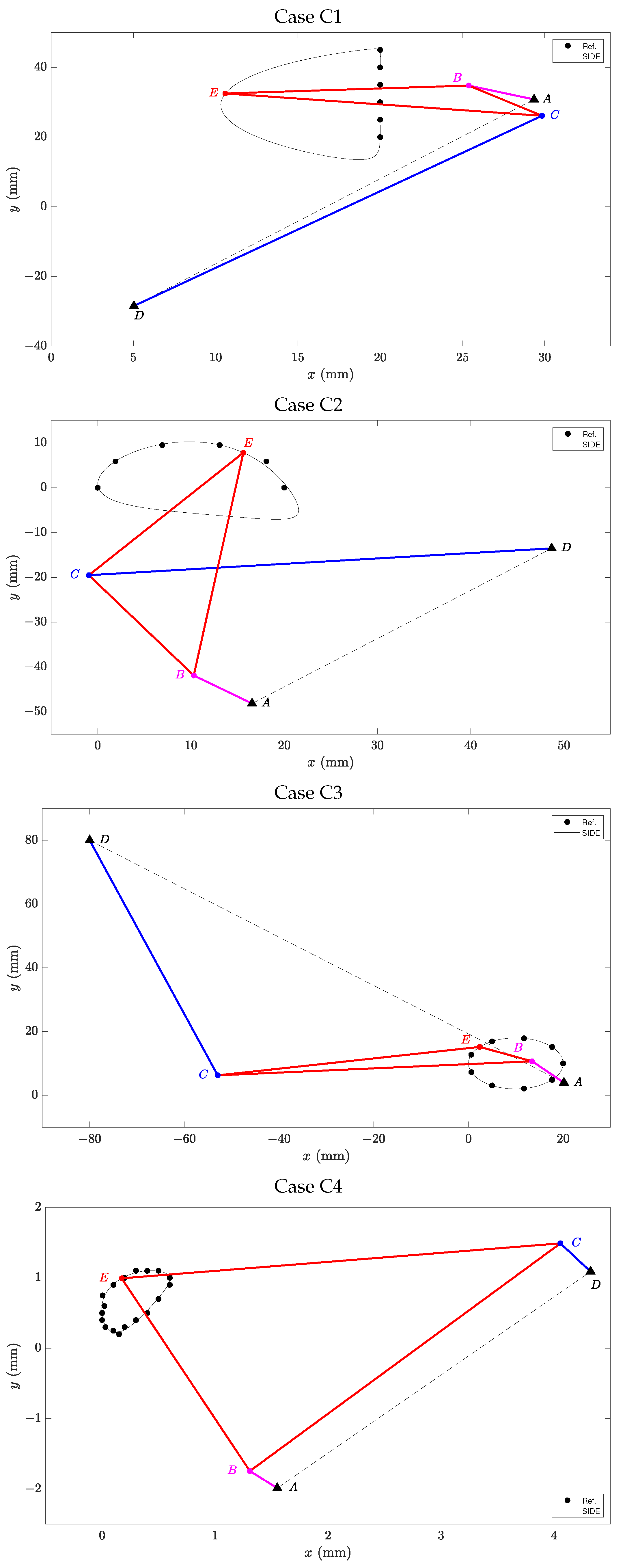
As with the rest of the DE variants studied, 30 independent runs were performed with the SIDE. For this, the parameters of the SIDE remained the same as those of the other DE variants studied.

Table 15. Results obtained with SIDE concerning the value of the objective function $J\left(\overrightarrow{p}\right)$ for each case study.

Case Study	Min $\mathit{J}\left(\overrightarrow{\mathit{p}}\right)$	Max $\mathit{J}\left(\overrightarrow{\mathit{p}}\right)$	Mean $\mathit{J}\left(\overrightarrow{\mathit{p}}\right)$	Std $\mathit{J}\left(\overrightarrow{\mathit{p}}\right)$
C1	3.3069 $\times {10}^{-27}$	4.7144 $\times {10}^{-2}$	4.2525 $\times {10}^{-3}$	1.0397 $\times {10}^{-2}$
C2	7.8637 $\times {10}^{-1}$	1.5482 $\times {10}^1$	8.1343	7.4736
C3	1.4870 $\times {10}^{-4}$	8.3759 $\times {10}^{-4}$	2.6975 $\times {10}^{-4}$	1.9250 $\times {10}^{-4}$
C4	1.0585 $\times {10}^{-2}$	2.5307 $\times {10}^{-2}$	1.5362 $\times {10}^{-2}$	4.8990 $\times {10}^{-3}$

shows the results obtained for each case study. The information contained in this table includes the same columns as Table 4, Table 5, Table 6 and Table 7. Shaded cells indicate results where the SIDE performed equal to or better than all other DE variants based on the information previously reported in Table 4, Table 5, Table 6 and Table 7. The main finding of this table is that the SIDE had an outstanding performance in half of the performance indicators. For the rest of the indicators, the SIDE showed a competitive performance. The best mechanisms synthesized by the SIDE and their developed trajectories are depicted in Figure 6 for all cases studies. The corresponding mechanism parameters can be consulted in the next Section 5.3.2.

The Wilcoxon test was also applied to the DE variants rand/1/exp, best/1/bin, and SIDE with statistical significance $\alpha =5\%$ to provide enough information about the algorithm performance. The test results are shown in

Table 16. Wilcoxon test results for the DE variants rand/1/exp, best/1/bin, and SIDE considering all case studies.

Test	Case C1	Case C2	Case C3	Case C4
best/1/bin vs. SIDE	$(-)$ 1.8626 $\times {10}^{-6}$	$(=)$ 6.5517 $\times {10}^{-1}$	$(-)$ 2.5518 $\times {10}^{-6}$	$(-)$ 1.8242 $\times {10}^{-6}$
best/1/bin vs. rand/1/exp	$(-)$ 1.8626 $\times {10}^{-6}$	$(=)$ 5.9408 $\times {10}^{-1}$	$(-)$ 5.7183 $\times {10}^{-6}$	$(-)$ 1.8626 $\times {10}^{-6}$
SIDE vs. rand/1/exp	$(=)$ 3.0852 $\times {10}^{-1}$	$(=)$ 1.0000	$(+)$ 8.3389 $\times {10}^{-3}$	$(=)$ 5.0840 $\times {10}^{-1}$

, and the summary of wins can be found in

Table 17. Summary of Wilcoxon test wins for the DE variants rand/1/exp, best/1/bin, and SIDE considering all case studies.

Variant	Case C1	Case C2	Case C3	Case C4	Total
best/1/bin	0	0	0	0	0
rand/1/exp	1	0	1	1	3
SIDE	1	0	2	1	4

. The formats of these two tables coincided with those of Table 13 and Table 14, respectively. Based on the information in Table 16, it is possible to determine that the SIDE had a performance that was comparable to that of best/1/bin for case C2 and that was better in the rest of the case studies. Concerning rand/1/exp, the performance of the SIDE is better in case C3, while there were no significant differences in the performance of these two variants for the other cases. The overall finding in the comparison results of the SIDE with respect to the two most outstanding DE variants based on Table 14 is that the SIDE tended to improve the search for solutions among the studied cases in comparison with the most outstanding DE variant, thereby increasing the likelihood that the problem would be solved successfully.

Concerning time,

Table 18. Results obtained with SIDE concerning the execution time t for each case study.

Case Study	Min $\mathit{J}\left(\overrightarrow{\mathit{p}}\right)$	Max $\mathit{J}\left(\overrightarrow{\mathit{p}}\right)$	Mean $\mathit{J}\left(\overrightarrow{\mathit{p}}\right)$	Std $\mathit{J}\left(\overrightarrow{\mathit{p}}\right)$
C1	1.9510	2.6320	2.3715	1.8188 $\times {10}^{-1}$
C2	2.1930	2.2840	2.2418	2.7821 $\times {10}^{-2}$
C3	3.6470	3.8430	3.7554	4.1968 $\times {10}^{-2}$
C4	4.0490	5.0110	4.6015	2.6940 $\times {10}^{-1}$

shows the minimum, maximum, mean, and standard deviation of the execution time t for the 30 independent runs of the SIDE for each case study. The values in gray indicate the cases where the SIDE outperformed the best results in Table 8, Table 9, Table 10 and Table 11. The statistical information on the execution times in this table did not present important differences with respect to what was reported in Table 8, Table 9, Table 10 and Table 11; thus, the SIDE was as efficient as the rest of the alternatives.

Finally,

Table 19. Minimum and maximum errors obtained with the best mechanism synthesized by SIDE for all case studies.

Case Study	Min e (mm)	Max e (mm)
C1	1.2041 $\times {10}^{-4}$	1.4047 $\times {10}^{-3}$
C2	7.9865 $\times {10}^{-2}$	6.1541 $\times {10}^{-1}$
C3	1.7193 $\times {10}^{-4}$	6.7010 $\times {10}^{-3}$
C4	1.8661 $\times {10}^{-1}$	6.9446 $\times {10}^{-1}$

shows the minimum and maximum error e values achieved with the best mechanisms synthesized by the SIDE for all case studies. The values in gray indicate that the error e obtained with the SIDE was better or at least equal to the best results in Table 12. Thus, this table indicates that the accuracy of the mechanisms obtained with the SIDE was competitive with respect to the best error values obtained with the rest of the variants of DE.

5.3.2. Comparative Results of SIDE with the State-of-the-Art Algorithms

After determining the effectiveness of the SIDE concerning the other DE variants studied in this work, the results were contrasted with those obtained by algorithms in recent specialized literature for the dimensional synthesis of four-bar Grashof-type mechanisms. The works in [26,35] were selected for this purpose. In [35], the dimensional synthesis of the four-bar mechanism was tackled with nine advanced optimization algorithms for six case studies, including those from the benchmark in [40]. On the other hand, the work in [26] proposed the dimensional synthesis of four-bar mechanisms through a parameterization based on a motion analysis with relative angles. This parameterization of the synthesis problem was solved through DE for five case studies, three of which corresponded to those of the benchmark in [40].

The best results obtained by the SIDE and by the algorithms used in [26,35] are presented in

Table 20. Best parameters obtained with SIDE in contrast to the best results in state-of-the-art algorithms for case study C1.

Variable (${\overrightarrow{\mathit{p}}}_{\mathit{j}}$)	SIDE	QO Rao-2 [35]	ODSRA + CP DE/best/1/bin [26]
$x_a$ ($\mathrm{mm}$)	29.3553	−11.9720	−27.7229
$y_a$ ($\mathrm{mm}$)	30.8045	60.0000	1.3008
$x_d$ ($\mathrm{mm}$)	5.0317	−47.3008	−31.9141
$y_d$ ($\mathrm{mm}$)	−28.4352	29.4142	25.6686
$l_2$ ($\mathrm{mm}$)	5.6144	10.3247	12.6721
$l_3$ ($\mathrm{mm}$)	9.7400	33.5451	29.4206
$l_4$ ($\mathrm{mm}$)	59.9210	60.0000	34.5589
$l_b$ ($\mathrm{mm}$)	14.9694	44.5702	58.6464
$q_b$ ($\mathrm{rad}$)	4.3897	0.0650	0.0027
$q_{2,1}$ ($\mathrm{rad}$)	5.4966	6.1793	4.5603
$q_{2,2}$ ($\mathrm{rad}$)	5.88292	6.6391	4.8417
$q_{2,3}$ ($\mathrm{rad}$)	6.22816	7.0533	5.1274
$q_{2,4}$ ($\mathrm{rad}$)	0.28671	7.4714	5.4181
$q_{2,5}$ ($\mathrm{rad}$)	0.654503	7.9238	5.7180
$q_{2,6}$ ($\mathrm{rad}$)	1.11249	8.4657	6.0407
$J\left(\overrightarrow{p}\right)$	3.3069 $\times {10}^{-27}$	1.3679 $\times {10}^{-4}$	1.0589 $\times {10}^{-5}$

,

Table 21. Best parameters obtained with SIDE in contrast to the best results in state-of-the-art algorithms for case study C2.

Variable (${\overrightarrow{\mathit{p}}}_{\mathit{j}}$)	SIDE	QO Rao-1 [35]
$x_a$ ($\mathrm{mm}$)	16.5532	10.2439
$y_a$ ($\mathrm{mm}$)	−48.1475	−3.8363
$x_d$ ($\mathrm{mm}$)	48.6904	60.2057
$y_d$ ($\mathrm{mm}$)	−13.5287	−5.7904
$l_2$ ($\mathrm{mm}$)	8.8474	1.4472
$l_3$ ($\mathrm{mm}$)	25.0467	1.4474
$l_4$ ($\mathrm{mm}$)	50.0000	50.0000
$l_b$ ($\mathrm{mm}$)	50.0000	12.3135
$q_b$ ($\mathrm{rad}$)	5.7108	0.3474
$J\left(\overrightarrow{p}\right)$	7.8637 $\times {10}^{-1}$	1.2254

Note: the prescribed time in Table 2 was increased by $q_{2,0}=6.2441$ for QO Rao-1.

,

Table 22. Best parameters obtained with SIDE in contrast to the best results in state-of-the-art algorithms for case study C3.

Variable (${\overrightarrow{\mathit{p}}}_{\mathit{j}}$)	SIDE	SAMP Rao-1 [35]	ODSRA + CP DE/best/1/bin [26]
$x_a$ ($\mathrm{mm}$)	20.1582	4.9497	11.5875
$y_a$ ($\mathrm{mm}$)	3.9543	16.4130	20.3173
$x_d$ ($\mathrm{mm}$)	−80.0000	81.7247	−63.4658
$y_d$ ($\mathrm{mm}$)	80.0000	−6.0726	47.7211
$l_2$ ($\mathrm{mm}$)	9.5007	8.8223	8.0705
$l_3$ ($\mathrm{mm}$)	66.5475	44.9536	49.8586
$l_4$ ($\mathrm{mm}$)	78.5406	47.6238	42.9186
$l_b$ ($\mathrm{mm}$)	11.9414	8.3934	10.4609
$q_b$ ($\mathrm{rad}$)	5.8299	−1.1323	−4.0483
$q_{2,1}$ ($\mathrm{rad}$)	6.1716	6.1876	6.3003
$q_{2,2}$ ($\mathrm{rad}$)	0.591315	6.8961	6.9958
$q_{2,3}$ ($\mathrm{rad}$)	1.30173	7.5968	7.7068
$q_{2,4}$ ($\mathrm{rad}$)	2.01028	8.2880	8.4197
$q_{2,5}$ ($\mathrm{rad}$)	2.71449	8.9621	2.8449
$q_{2,6}$ ($\mathrm{rad}$)	3.41391	9.6439	3.5525
$q_{2,7}$ ($\mathrm{rad}$)	4.10476	10.3350	4.2469
$q_{2,8}$ ($\mathrm{rad}$)	4.79219	11.0451	4.9363
$q_{2,9}$ ($\mathrm{rad}$)	5.4767	11.7562	5.6147
$q_{2,10}$ ($\mathrm{rad}$)	6.1716	6.1876	6.3002
$J\left(\overrightarrow{p}\right)$	1.4870 $\times {10}^{-4}$	9.5753 $\times {10}^{-4}$	5.8199 $\times {10}^{-4}$

and

Table 23. Best parameters obtained with SIDE in contrast to the best results in state-of-the-art algorithms for case study C4.

Variable (${\overrightarrow{\mathit{p}}}_{\mathit{j}}$)	SIDE	QO Rao-1 [35]	ODSRA + CP DE/best/1/bin [26]
$x_a$ ($\mathrm{mm}$)	1.5505	0.5825	0.2624
$y_a$ ($\mathrm{mm}$)	−1.9868	0.7537	0.1439
$x_d$ ($\mathrm{mm}$)	4.3235	−4.3189	1.2617
$y_d$ ($\mathrm{mm}$)	1.0883	−0.2345	0.4936
$l_2$ ($\mathrm{mm}$)	0.3430	0.3383	0.4255
$l_3$ ($\mathrm{mm}$)	4.2439	0.5786	0.9446
$l_4$ ($\mathrm{mm}$)	0.4821	4.7770	0.5779
$l_b$ ($\mathrm{mm}$)	2.9631	0.3934	0.5539
$q_b$ ($\mathrm{rad}$)	1.0974	−0.9996	0.7932
$q_{2,0}$ ($\mathrm{rad}$)	1.2852	6.8211	1.1743
$J\left(\overrightarrow{p}\right)$	1.0585 $\times {10}^{-2}$	1.2904 $\times {10}^{-2}$	9.9134 $\times {10}^{-3}$

for each case study. The columns of these tables show the values of the design variables calculated with each algorithm, while the value of the objective function $J\left(\overrightarrow{p}\right)$ achieved with them is noted at the bottom. The best synthesis of the four-bar mechanism for each case study is highlighted in gray. Based on the information in these tables, it is possible to observe that the results obtained by the SIDE were superior in all four case studies compared to those of [26,35], except for case C4, where it was outperformed by the work on [26] but was still competitive. This highlights the value of this study as a basis for proposing advanced algorithms with a greater capacity to solve complex problems related to the synthesis of mechanisms. At this point, it is important to note that the configuration of the hyperparameters in the SIDE and in the algorithms of the papers [26,35] are different. While in [26], the algorithms were set up to perform a similar number of evaluations of the optimization problem reported in the literature, the configuration of the algorithms in [35] were oriented to reduce this number considerably. The main aim of the SIDE was to provide a four-bar mechanism oriented to accurately develop the task, which would impact future engineering applications, i.e., accuracy was the most important criterion, thereby sacrificing the number of times that the performance function was evaluated. Of course, a reduced number of evaluations implies shorter execution times. However, the execution times achieved with the SIDE were relatively small (see Table 18) when contrasted with the effective syntheses of the obtained four-bar mechanism (see Table 15).

6. Conclusions and Future Work

Four-bar Grashof-type mechanisms are mechanical systems used in various important real-world applications and form the basis of much more complex mechanisms. The dimensional synthesis of these mechanisms is a challenging problem that can be stated as one of global optimization with constraints. Metaheuristic optimization techniques, especially Differential Evolution (DE), can provide good solutions to this problem at an affordable computational cost. The great diversity of DE variants makes it impossible to experiment with all of them on the synthesis problem to determine the most promising alternative. The study developed in this work made it possible to evaluate and compare the performance of the most used variants of DE in the solution of the mechanism synthesis problem. Based on an analysis with non-parametric and descriptive statistics, it was determined that the variant rand/1/exp could obtain outstanding results in the solution of the two conceptualizations of the synthesis problem (i.e., with and without prescribed time). This is attributed to the exploratory capability of the rand variants and the ability of the exp crossover operator to obtain suitable solutions as the number of design variables increases. To illustrate the usefulness of the study, a Simple and Improved DE (SIDE) variant was proposed that was based on the best-performing alternatives, i.e., rand/1/exp and best/1/bin. The SIDE showed higher performance in solving the case studies addressed in this work. In addition, the SIDE showed better performance with respect to the results reported in the recent literature for the same case studies in terms of more accurate tracking of the precision points without limiting the number of evaluations of the optimization problem. This may have positive benefits from a practical engineering point of view. The results obtained from this study are expected to support the development of more efficient algorithms based on DE rand/1/exp and to serve as a guide for solving more specific case studies in the future. Future work also involves the comparative analysis of the SIDE for solving the spatial mechanism synthesis problem. Moreover, as a further step after the dimensional synthesis of the four-bar mechanism, the dynamic modeling of the mechanism for simulation [48] and control law design [49] is intended to be studied in the future under metaheuristic optimization approaches.

The main aim of the SIDE is to provide a four-bar mechanism oriented to accurately develop the task which will impact future engineering applications, i.e., accuracy is the most important criterion, thereby sacrificing the number of times that the performance function is evaluated.

References

1. Sousa, M.J.; Wilks, D. Sustainable Skills for the World of Work in the Digital Age. Syst. Res. Behav. Sci. 2018, 35, 399–405. [Google Scholar] [CrossRef]
2. Norton, R.L. Design of Machinery: An Introduction to the Synthesis and Analysis of Mechanisms and Machines; McGraw-Hill/Higher Education: New York, NY, USA, 2008. [Google Scholar]
3. Xu, L.J. Simulation Analysis about Dynamic Characteristics of Four-Bar Linkage Portal Crane’s Jib Based on the Lifting Loads. In Proceedings of the 2015 Sixth International Conference on Intelligent Systems Design and Engineering Applications (ISDEA), Guiyang, China, 18–19 August 2015; pp. 719–722. [Google Scholar] [CrossRef]
4. Qu, X.; Kim, D. Kinematic design and analysis of a four-bar linkage-type continuously variable valve actuation mechanism. Mech. Mach. Theory 2012, 57, 111–125. [Google Scholar] [CrossRef]
5. Singla, A.; Singh, G.; Virk, G.S. Matlab/simMechanics based control of four-bar passive lower-body mechanism for rehabilitation. Perspect. Sci. 2016, 8, 351–354. [Google Scholar] [CrossRef] [Green Version]
6. Ishihara, H. Compliant and compact joint mechanism for a child android robot. In Proceedings of the 2016 11th ACM/IEEE International Conference on Human-Robot Interaction (HRI), Christchurch, New Zealand, 7–10 March 2016; pp. 553–554. [Google Scholar] [CrossRef]
7. Wang, D.; Wu, J.; Wang, L.; Liu, Y. A Postprocessing Strategy of a 3-DOF Parallel Tool Head Based on Velocity Control and Coarse Interpolation. IEEE Trans. Ind. Electron. 2018, 65, 6333–6342. [Google Scholar] [CrossRef]
8. Singh, A.R.; Dixit, A.; Dhupal, J. Finite element analysis of case box tape sealer mechanism. Mater. Today Proc. 2020, 25, 570–576. [Google Scholar] [CrossRef]
9. Gogu, G. Structural Synthesis of Parallel Robots: Part 3: Topologies with Planar Motion of the Moving Platform; Springer Science & Business Media: Berlin/Heidelberg, Germany, 2010; Volume 173. [Google Scholar]
10. Spong, M.W.; Hutchinson, S.; Vidyasagar, M. Robot Modeling and Control; John Wiley & Sons: Hoboken, NJ, USA, 2020. [Google Scholar]
11. Bourbonnais, F.; Bigras, P.; Bonev, I.A. Minimum-Time Trajectory Planning and Control of a Pick-and-Place Five-Bar Parallel Robot. IEEE/ASME Trans. Mechatron. 2015, 20, 740–749. [Google Scholar] [CrossRef]
12. Campos, A.; Budde, C.; Hesselbach, J. A type synthesis method for hybrid robot structures. Mech. Mach. Theory 2008, 43, 984–995. [Google Scholar] [CrossRef]
13. Bergelin, B.J.; Voglewede, P.A. Design of an Active Ankle-Foot Prosthesis Utilizing a Four-Bar Mechanism. J. Mech. Des. 2012, 134, 061004. [Google Scholar] [CrossRef]
14. Sitti, M. Piezoelectrically actuated four-bar mechanism with two flexible links for micromechanical flying insect thorax. IEEE/ASME Trans. Mechatron. 2003, 8, 26–36. [Google Scholar] [CrossRef] [Green Version]
15. Liaw, H.C.; Shirinzadeh, B.; Smith, J. Robust motion tracking control of piezo-driven flexure-based four-bar mechanism for micro/nano manipulation. Mechatronics 2008, 18, 111–120. [Google Scholar] [CrossRef]
16. Hosseini, H.; Farzad, A.; Majeed, F.; Hensel, O.; Nasirahmadi, A. Multi-Objective Optimal Design and Development of a Four-Bar Mechanism for Weed Control. Machines 2022, 10, 198. [Google Scholar] [CrossRef]
17. Barker, C.R. A complete classification of planar four-bar linkages. Mech. Mach. Theory 1985, 20, 535–554. [Google Scholar] [CrossRef]
18. Lee, W.T.; Russell, K. Developments in quantitative dimensional synthesis (1970-present): Four-bar motion generation. Inverse Probl. Sci. Eng. 2018, 26, 133–148. [Google Scholar] [CrossRef]
19. Varedi-Koulaei, S.; Rezagholizadeh, H. Synthesis of the four-bar linkage as path generation by choosing the shape of the connecting rod. Proc. Inst. Mech. Eng. Part C J. Mech. Eng. Sci. 2020, 234, 2643–2652. [Google Scholar] [CrossRef]
20. Huang, X.; Liao, Q.; Wei, S.; Xu, Q. Five precision point-path synthesis of planar four-bar linkage using algebraic method. Front. Electr. Electron. Eng. China 2008, 3, 470–474. [Google Scholar] [CrossRef]
21. Ebrahimi, S.; Payvandy, P. Efficient constrained synthesis of path generating four-bar mechanisms based on the heuristic optimization algorithms. Mech. Mach. Theory 2015, 85, 189–204. [Google Scholar] [CrossRef]
22. Kang, Y.H.; Lin, J.W.; You, W.C. Comparative Study on the Synthesis of Path-Generating Four-Bar Linkages Using Metaheuristic Optimization Algorithms. Appl. Sci. 2022, 12, 7368. [Google Scholar] [CrossRef]
23. Waghmare, G.G.; Rao, R.V.; Kulkarni, P.C. Path synthesis of a four-bar linkage using a teaching-learning-based optimization algorithm. Int. J. Comput. Methods Eng. Sci. Mech. 2023, 24, 40–51. [Google Scholar] [CrossRef]
24. Grabski, J.K.; Sopa, M.; Mrozek, A. Application of the path-repairing technique and virus optimization algorithm for the dimensional synthesis of four-bar mechanisms. Arch. Civ. Mech. Eng. 2023, 23, 134. [Google Scholar] [CrossRef]
25. Muñoz-Reina, J.S.; Villarreal-Cervantes, M.G.; Corona-Ramírez, L.G.; Valencia-Segura, L.E. Neuronal Constraint-Handling Technique for the Optimal Synthesis of Closed-Chain Mechanisms in Lower Limb Rehabilitation. Appl. Sci. 2022, 12, 2396. [Google Scholar] [CrossRef]
26. Valencia-Segura, L.E.; Villarreal-Cervantes, M.G.; Corona-Ramírez, L.G.; Cuenca-Jiménez, F.; Castro-Medina, R. Optimum Synthesis of Four-Bar Mechanism by Using Relative Angle Method: A Comparative Performance Study. IEEE Access 2021, 9, 132990–133010. [Google Scholar] [CrossRef]
27. Reeves, C.R. (Ed.) Modern Heuristic Techniques for Combinatorial Problems; John Wiley & Sons, Inc.: Hoboken, NJ, USA, 1993. [Google Scholar]
28. Alorf, A. A survey of recently developed metaheuristics and their comparative analysis. Eng. Appl. Artif. Intell. 2023, 117, 105622. [Google Scholar] [CrossRef]
29. Anosri, S.; Panagant, N.; Champasak, P.; Bureerat, S.; Thipyopas, C.; Kumar, S.; Pholdee, N.; Yıldız, B.S.; Yildiz, A.R. A Comparative Study of State-of-the-art Metaheuristics for Solving Many-objective Optimization Problems of Fixed Wing Unmanned Aerial Vehicle Conceptual Design. Arch. Comput. Methods Eng. 2023. [Google Scholar] [CrossRef]
30. Price, K.; Storn, R.M.; Lampinen, J.A. Differential Evolution: A Practical Approach to Global Optimization (Natural Computing Series); Springer: Berlin/Heidelberg, Germany, 2005. [Google Scholar]
31. Sancibrian, R.; Sedano, A.; Sarabia, E.G.; Blanco, J.M. Hybridizing differential evolution and local search optimization for dimensional synthesis of linkages. Mech. Mach. Theory 2019, 140, 389–412. [Google Scholar] [CrossRef]
32. Nguyen-Van, S.; Lieu, Q.X.; Xuan-Mung, N.; Nguyen, T.T.N. A New Study on Optimization of Four-Bar Mechanisms Based on a Hybrid-Combined Differential Evolution and Jaya Algorithm. Symmetry 2022, 14, 381. [Google Scholar] [CrossRef]
33. Zhang, K.; Huang, Q.; Zhang, Y.; Song, J.; Shi, J. Hybrid Lagrange interpolation differential evolution algorithm for path synthesis. Mech. Mach. Theory 2019, 134, 512–540. [Google Scholar] [CrossRef]
34. Villarreal-Cervantes, M.G.; Pantoja-García, J.S.; Rodríguez-Molina, A.; Benitez-Garcia, S.E. Pareto optimal synthesis of eight-bar mechanism using meta-heuristic multi-objective search approaches: Application to bipedal gait generation. Int. J. Syst. Sci. 2021, 52, 671–693. [Google Scholar] [CrossRef]
35. Rao, R.; Pawar, R. Dimensional synthesis of four-bar mechanisms using Rao algorithms and their variants. Appl. Soft Comput. 2023, 132, 109839. [Google Scholar] [CrossRef]
36. Caraffini, F.; Santucci, V.; Milani, A. Evolutionary Computation & Swarm Intelligence; MDPI: Basel, Switzerland, 2020. [Google Scholar]
37. Mezura-Montes, E.; Velázquez-Reyes, J.; Coello Coello, C.A. A Comparative Study of Differential Evolution Variants for Global Optimization. In Proceedings of the 8th Annual Conference on Genetic and Evolutionary Computation, Association for Computing Machinery, New York, NY, USA, 8–12 July 2006; GECCO ’06. pp. 485–492. [Google Scholar] [CrossRef] [Green Version]
38. Deb, K. An efficient constraint handling method for genetic algorithms. Comput. Methods Appl. Mech. Eng. 2000, 186, 311–338. [Google Scholar] [CrossRef]
39. Opara, K.R.; Arabas, J. Differential Evolution: A survey of theoretical analyses. Swarm Evol. Comput. 2019, 44, 546–558. [Google Scholar] [CrossRef]
40. Lin, W.Y. A GA–DE hybrid evolutionary algorithm for path synthesis of four-bar linkage. Mech. Mach. Theory 2010, 45, 1096–1107. [Google Scholar] [CrossRef]
41. Wei, W.; Shu, X.; Chen, P.; Li, X. A chord-angle-based approach with expandable solution space to 1-degree-of-freedom (DOF) rehabilitation mechanism synthesis. Mech. Sci. 2022, 13, 341–352. [Google Scholar] [CrossRef]
42. Jeyakumar, G.; Shunmuga Velayutham, C. Hybridizing Differential Evolution Variants Through Heterogeneous Mixing in a Distributed Framework. In Hybrid Soft Computing Approaches: Research and Applications; Bhattacharyya, S., Dutta, P., Chakraborty, S., Eds.; Springer: New Delhi, India, 2016; pp. 107–151. [Google Scholar] [CrossRef]
43. Zhao, S.Z.; Suganthan, P.N. Empirical investigations into the exponential crossover of differential evolutions. Swarm Evol. Comput. 2013, 9, 27–36. [Google Scholar] [CrossRef]
44. Bataller, A.; Cabrera, J.; Clavijo, M.; Castillo, J. Evolutionary synthesis of mechanisms applied to the design of an exoskeleton for finger rehabilitation. Mech. Mach. Theory 2016, 105, 31–43. [Google Scholar] [CrossRef]
45. Calva-Yáñez, M.B.; Niño-Suarez, P.A.; Portilla-Flores, E.A.; Aponte-Rodríguez, J.A.; Santiago-Valentn, E. Reconfigurable Mechanical System Design for Tracking an Ankle Trajectory Using an Evolutionary Optimization Algorithm. IEEE Access 2017, 5, 5480–5493. [Google Scholar] [CrossRef]
46. Singh, R.; Chaudhary, H.; Singh, A.K. A Novel Gait-Inspired Four-Bar Lower Limb Exoskeleton To Guide The Walking Movement. J. Mech. Med. Biol. 2019, 19, 1950020. [Google Scholar] [CrossRef]
47. Derrac, J.; García, S.; Molina, D.; Herrera, F. A practical tutorial on the use of nonparametric statistical tests as a methodology for comparing evolutionary and swarm intelligence algorithms. Swarm Evol. Comput. 2011, 1, 3–18. [Google Scholar] [CrossRef]
48. Arian, A.; Isaksson, M.; Gosselin, C. Kinematic and dynamic analysis of a novel parallel kinematic Schönflies motion generator. Mech. Mach. Theory 2020, 147, 103629. [Google Scholar] [CrossRef]
49. Mohan, S.; Mohanta, J.; Kurtenbach, S.; Paris, J.; Corves, B.; Huesing, M. Design, development and control of a 2PRP-2PPR planar parallel manipulator for lower limb rehabilitation therapies. Mech. Mach. Theory 2017, 112, 272–294. [Google Scholar] [CrossRef]
50. Mohan Rao, A.V.; Sandor, G.N. Extension of Freudenstein’s Equation to Geared Linkages. J. Eng. Ind. 1971, 93, 201–210. [Google Scholar] [CrossRef]
Figure 1. Schematic diagram of the four-bar mechanism.
Applsci 13 06966 g001
Figure 2. Best trajectories generated by each DE variant for case study C1.
Applsci 13 06966 g002
Figure 3. Best trajectories generated by each DE variant for case study C2.
Applsci 13 06966 g003
Figure 4. Best trajectories generated by each DE variant for case study C3.
Applsci 13 06966 g004
Figure 5. Best trajectories generated by each DE variant for case study C4.
Applsci 13 06966 g005
Figure 6. Best mechanisms synthesized by SIDE for all case studies. The corresponding mechanism parameters can be consulted in the next Section 5.3.2.
Applsci 13 06966 g006