Featured Application
Telepresence robot is useful for remote applications, healthcare and remote sensing.
Abstract
Automation in the modern world has become a necessity for humans. Intelligent mobile robots have become necessary to perform various complex tasks in healthcare and industry environments. Mobile robots have gained attention during the pandemic; human–robot interaction has become vibrant. However, there are many challenges in obtaining human–robot interactions regarding maneuverability, controllability, stability, drive layout and autonomy. In this paper, we proposed a stability and control design for a telepresence robot called auto-MERLIN. The proposed design simulated and experimentally verified self-localization and maneuverability in a hazardous environment. A model from Rieckert and Schunck was initially considered to design the control system parameters. The system identification approach was then used to derive the mathematical relationship between the manipulated variable of robot orientation control. The theoretical model of the robot mechanics and associated control were developed. A design model was successfully implemented, analyzed mathematically, used to build the hardware and tested experimentally. Each level takes on excellent tasks for the development of auto-MERLIN. A higher level always uses the services of lower levels to carry out its functions. The proposed approach is comparatively simple, less expensive and easily deployable compared to previous methods. The experimental results showed that the robot is functionally complete in all aspects. A test drive was performed over a given path to evaluate the hardware, and the results were presented. Simulation and experimental results showed that the target path is maintained quite well.
1. Introduction
In the recent era, mobile robots are receiving attention in many applications where human and robot interactions have become feasible. In addition, the application of robots in a friendly manner and the simplicity of the robotic design complement humans in many activities. Everyone is talking about smartness and digitization in daily and routine life. The demand for automation is increasing daily, with greater flexibility in completing tasks. There are many research gaps and applications of the telepresence robot. A few of the research gaps are highlighted as follows:
- Robots can work remotely and even in environments where it becomes impossible for a human being to approach them. These robots are obtaining market value due to their capabilities, including executing complex tasks simply and with a fast and precise response. It becomes easy for the robot to work in hazardous environments [1,2,3].
- Besides completing complex tasks, robots are mostly used in entertainment, the fashion industry, teleconferencing and healthcare systems [4,5,6]. However, healthcare applications require sophisticated robots to perform exact and precise surgery, which requires complex robot design and controlled functions [7]. For such an environment, robots should be well-trained using the master–slave application. In other environments, such as military applications and a scenario such as the COVID-19 pandemic, orientation and self-localization play a vital role.
- In the current situation, human beings are more dependent on technology than ever before, and it is becoming more and more complicated. Even though rapid progress in automation has been attained in addressing social and industrial issues using remotely controlled devices, further investigation is inspired by user satisfaction and systematic requirement analysis. Telepresence robots, called smart and independent machines, could be a possible substitute to be included in the human social ecosystem. Telepresence robots are machines designed to enable individuals to interact with and explore remote environments in real time. These robots can be remotely operated from anywhere worldwide, allowing users to virtually visit far-flung locations without leaving the comfort of their homes or offices [8]. It is accessible as a reasonable solution, permitting the user to be at home with ongoing distant checking and maintain communication with the counsellor [9,10,11]. The concept of telepresence has been around for decades. Still, recent advancements in technology have made it possible to create more sophisticated telepresence robots that offer a higher degree of interactivity and immersion. These robots typically consist of a mobile base that can move around a space, a camera and microphone for capturing video and audio, and a screen or display that allows the user to see and hear what the robot is seeing and hearing. [12,13].
In the presented research work, a stability and control design of a mobile robot has been developed. One of the primary applications of telepresence robots is in the field of remote work. With the rise in remote work and distributed teams, telepresence robots offer a way for remote workers to feel more connected to their colleagues and workplace. For example, a telepresence robot can allow remote workers to attend meetings and interact with coworkers as if they were physically in the office [14,15,16,17,18,19]. Telepresence robots are also increasingly being used in healthcare settings. For example, doctors can use telepresence robots to remotely visit patients and provide consultations without physically being in the same location. This is particularly useful for patients in remote or underserved areas, where access to medical professionals may be limited. A mini-computer is an essential part of the robot, which comprises the user program, and the operator can parameterize the robot by exploiting these parameters. A wireless interface is also applied so the robot can be operated remotely [20].
A small robot model referred to as HPI Savage 2.1 was established, as shown in Figure 1. The vehicle is furnished with Ackermann steering and is controlled on a double track, meaning the robot can be controlled with front wheels. It is a four-wheel drive, and full control is available on each wheel to steer in any direction and control the motion. Thus, similar settings conquer as in an ordinary four-wheel-drive vehicle. It monitors that the speed and maneuverability of the robot are coupled.
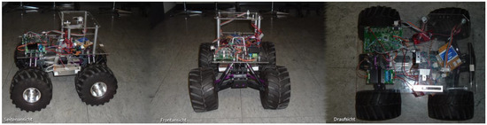
Figure 1.
Attached robot on the Monster Truck HPI Savage 2.1.
The robot exploits three heavy-duty direct current (DC) motors called TruckPuller3 of 7.2 V each and the controlling-model-equipped servo motor HiTec HS-5745MG. An optical position encoder M101B of Megatron Elektronik AG & Co. is employed to drive the motor. In the era of automation, telepresence robots are becoming more attractive in various fields of medicine, academia and industries [20,21]. Each environment has different protocols to maximize performance and minimize security threats. In [22], the authors devised methods to enhance security in IoT-enabled environments. Secure routing planning methods have been suggested by [23,24]. The authors of [25] proposed new ideas to achieve adaptive and robust control for teleoperation. Many researchers have developed efficient mobile robot methods for the wireless sensor network in different scenarios, e.g., underwater and energy-aware cluster-based schemes [26,27,28,29,30]. The list of technical parameters of auto-MERLIN is given in Table 1.

Table 1.
Technical parameters of auto-MERLIN.
For autonomous navigation, orientation control is crucial; otherwise, the robot cannot reach its target goal point from the start. Therefore, the main focus was to design a precise and accurate orientation controller for an approximated robot model. A cascade control loop was developed where the speed controller out is fed to the position controller. Its output serves as an input to the orientation controller. The relationship between change in orientation and the PWM controller has been established mathematically. The results shown in Section 4 present the effectiveness of the designed controller through different scenarios. There is a very small drift between the actual orientation and the desired one due to the nonlinearity of stiffness of the steering mechanism. Most mobile robots have a differential drive, so it is easier to control orientation, unlike auto-MERLIN, a car-like robot with a nonlinear steering mechanism.
Orientation control of a mobile robot refers to the ability of the robot to adjust and maintain its direction of motion. This can be achieved through various techniques, such as using sensors to detect the robot’s orientation, implementing feedback control algorithms to adjust the robot’s motion and using mapping and localization techniques to track the robot’s position and orientation. Ultimately, orientation control ensures the robot can navigate its environment and complete its intended tasks.
The orientation control of a car-like mobile robot with a steering mechanism is essential to its navigation system. The robot’s orientation refers to the direction in which it is facing and moving. It is important to accurately control the robot’s orientation to achieve efficient and precise navigation. This article discusses the orientation control of a car-like mobile robot with a steering mechanism.
Firstly, let us understand the steering mechanism of a car-like mobile robot. The steering mechanism consists of two wheels at the front and two wheels at the back of the robot. The front wheels are connected to a steering mechanism that allows them to turn in different directions. By turning the front wheels, the robot can change its direction of movement. The back wheels propel the robot and keep it moving in a straight line.
To control the robot’s orientation, it is necessary to control the movement of the front wheels. The movement of the front wheels determines the direction of movement of the robot. The robot’s orientation can be controlled by changing the angle of the front wheels. This can be done using a servo motor connected to the robot’s steering mechanism. The servo motor can be controlled using a microcontroller that receives input from various sensors.
Various sensors can be used to control the orientation of the robot. These include gyroscopes, accelerometers and magnetometers. A gyroscope measures the robot’s rotation rate, while an accelerometer measures its acceleration. A magnetometer measures the magnetic field around the robot. Using these sensors, the microcontroller can determine the robot’s current orientation and adjust the angle of the front wheels accordingly.
The orientation control of a car-like mobile robot with a steering mechanism is crucial for its navigation system. By accurately controlling the robot’s orientation, it can move efficiently and precisely toward its target. This is particularly important in applications such as autonomous vehicles, where the robot must navigate complex environments without human intervention. The importance and contribution of the proposed research work is given below:
- The objective was to equip auto-MERLIN to navigate the desired path, sense obstacles and escape them. It needs advanced control electronics to be produced because the existing design did not fulfil the requirements.
- An important aspect of its navigation system is the orientation control of a car-like mobile robot with a steering mechanism.
- By controlling the movement of the front wheels, the robot’s orientation can be controlled. This can be achieved using sensors and a microcontroller that adjusts the angle of the front wheels.
- Efficiently and accurately navigate the robot toward its destination should be carried out with precise orientation control.
- A more sophisticated approach of self-localization and orientation control of the mobile robot is a dire requirement in the healthcare environment, which is discussed in this paper.
2. Background
Implementing a mobile robot in a healthcare environment is a crucial task. It is quite important for healthcare directors and policy makers [31]. It is also as much a concern for patients and operators who must operationalize them outside formal clinical situations [32,33]. It is worth mentioning that mobile robots are often considered the best alternative to explore and implement in aggressive remote areas. Conventional application regions are space examination and treating plants [8]. With the same consideration of exploration, modernized ideas have been explored in the healthcare system and industries [34]. The methodology and the design implementation remain the same to control the mobile robot in a healthcare environment [16,35]. The recent era of telematics, developed by employing internet service providers, enables the technology over a wide range of commercially available applications. Examples include telemedicine, equipment telemaintenance and online learning environments from remote locations [36].
Another application of telepresence robots is in education. With the rise of online learning, telepresence robots offer a way for students to participate in classroom discussions and interact with their peers and teachers as if they were physically present. This can be particularly helpful for students who cannot attend in-person classes due to illness or disability. Telepresence robots are also used in various other settings, such as museums, trade shows and even as personal assistants for individuals with disabilities. As technology advances, we will likely see even more innovative applications of telepresence robots in the future [37,38,39,40].
The most common approaches to the simple design of mobile robots can be found in [41,42]. A robot comprises both software and hardware designs. There are many components which provide much information about the motion and position of the mobile robot. The sensors fulfil the task and send the information to the remote operator to perform specific routine instructions. All this information is controlled using the software module of the robot [43,44]. The software part of the mobile robot sends the control instructions, which are operator-dependent. These are used to exactly control and locate the robot in the desired location and obtain important information from each actuator. The function of the actuator is to provide complete control over the hardware activities of the mobile robot [8,10,44]. The core concern of the design is to control the driving behavior and avoid an obstacle at each instance [6,38,45]. The second crucial part is the decision-making device, which controls the orientation robot and self-localizes it to avoid obstacles during the journey and provide a safe track [46,47]. Another term, “maneuver,” is also called, but better and more precise terms are “behavior” or localization, which are more frequently used in the article [48,49,50,51,52]. The control of a robot in an austere and cognitive environment is presented in [52,53]. More examples of ray robots with a multi-objective design are presented in [54,55].
3. Orientation Controller Design
The orientation controller controls the orientation of the robot. Adjusting this controller is a huge challenge because the distance can only be determined through rough estimates. Figure 2 shows the basic control loop of the orientation controller.
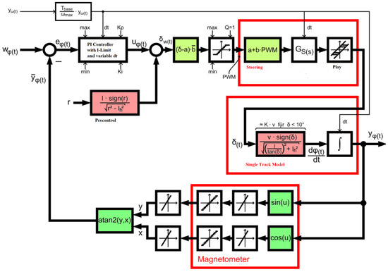
Figure 2.
Robot orientation controller.
The most important property of the controller is the variable time base. There is a base time constant Tbase set equal to the cycle time of the control algorithm. It is, therefore, 10 ms here. To determine the desired modified cycle time dt, this time base is multiplied by the ratio between the instantaneous drive speed and the maximum drive speed [45,50,51,52,53,54,55]. This is because the controller can be set for a constant driving speed of the robot, namely . With this modification, integrations are no longer carried out over time but over the distance covered. This makes sense because the robot’s orientation can only change when driving. It is impossible to change orientation when stationary, no matter how hard one steers. However, the variable time base also has some disadvantages for the controller [49,50,51,52,53].
On the one hand, only a PI controller can be used because the D component, when stationary, leads to a singularity due to division by zero. For this reason, the program implements the PI controller as a parallel connection of proportional and integral parts. However, no anti-wind-up feedback can be integrated. As a compromise, the integrator value accumulation is strictly limited.
Some blocks have been colored in the block diagram of the orientation control loop. Blocks of the same color largely compensate for each other. In principle, the controlled system consists of the red boxes’ steering and single-track model. The single-track model by Rieckert and Schunck was considered the first to model the controlled system. The steering behavior of the robot was then experimentally determined to derive the mathematical relationship between the manipulated variable of the steering servo and the robot orientation.
3.1. The Single-Track Model
First, the single-track model by Rieckert and Schunck for small velocities and accelerations was considered. The slippage of the vehicle due to centrifugal forces was neglected. Figure 3 shows the geometric relationships of the single-track model used here.
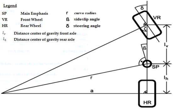
Figure 3.
Simplified single-track model from Rieckert and Schunck.
The single-track model (Riekert and Schunck) permits the approximation of the vehicle lateral dynamics, as shown in Figure 3. Utilizing it makes some simplifications possible without influencing the fundamental analysis of mobile robot behavior for lateral dynamics. Readers are encouraged to study for a more detailed implementation of the Riekert and Schunck model [56]. In the proposed case, we consider the static obstacles. The single-track model analysis explains the analysis of handling the mobile robot during the ride from the doctor’s office to the patient ward, and the behaviors of the wheels are observed during the track. By employing this model, it is easy to translate it into the simulation tool. Secondly, it is mostly employed because of simplicity and linear dependency between the wheel forces and the slip angle. The utilization of this model in the proposed research problem is based on some simplification about the slip angle, wheel forces, wheel-load distribution and longitudinal forces.
Figure 3 shows the geometric relationships of the single-track model. Figure 3 describes the following parameters: , and . The sideslip angle denotes the vehicle’s deviation direction from the center of gravity.
The current velocity of the front wheels is denoted over a fixed coordinate system and the steering angle . The vehicle’s movement relates to the vehicle’s center of gravity SP. When cornering with a constant steering angle , it describes a circular path with the curve radius . The relationship between the steering angle δ and the curve radius is sought. For this purpose, the right-angled triangle with sides , and is considered first. Side can be determined using the Pythagorean theorem.
Now, the right-angled triangle consisting of sides and and the angle ζ is considered. The tangent of angle ζ can be expressed using the two well-known legs of the triangle.
By inserting Equation (1) for , we obtain
The auxiliary angle ζ and the steering angle δ add up to a right angle π/2. Thus, the steering angle δ as
Substituting the value of in Equation (3).
Finally, Equation (5) can still use two identities
and
to
Now, there are two levels of approximation. First, can be neglected for the small steering angles .
If the curve radius is very large compared to the distance between the center of gravity and the rear axle, the term is simplified as follows:
According to Equation (10), the robot implements simple approximation because it delivers significantly better results than strong approximation. It should also be noted that only positive curve radii and steering angles are considered here. The information for steering to the left and right can be stored in the sign of the curve radius and the steering angle . For the robot, a positive sign means steering to the right, and a negative sign means steering to the left.
Now, the change in orientation is of interest as its integration gives the orientation angle . Because steering provides a steering angle , a function is sought that establishes a relationship between the steering angle and the change in orientation .
The change in orientation is angular velocity with path velocity and the circle radius . Thus, the change in orientation can be denoted as follows:
where is
Insert the radius into Equation (11) to obtain the following:
A functional connection between the steering angle and the change in orientation is therefore established.
3.2. Determination of the Steering Mechanics
The controlled system can now be modelled with the knowledge gained from the single-track model. The entire steering train should provide a steering angle , resulting in a sideslip angle or curve radius . The steering, which consists of the servo motor and the steering linkage, converts a PWM signal into a steering angle . This transmission element is considered to be linear. The relationship is determined experimentally. The vehicle translates the steering angle into a curve radius via the underlying single-track model, which is directly related to the change in orientation . This relationship is mathematically precisely defined from the previous consideration.
The mathematical function between the steering value PWM and the steering angle δ was determined experimentally. For this purpose, the steering value of the robot was set to specified values. After selecting the steering value, it had to be ensured that the wheels also assumed the associated steering angle. This can be seen from the fact that the steering servo made no more correction attempts. The robot slowly moved forward, and the path covered was recorded. In this case, the recording was done with a felt-tip pen that drew on the floor. The floor was previously laid out extensively with counting paper. Finally, the tracks were measured. The curve radius was determined from three measuring points per lane. The additional measurement points were intended to verify the calculated circle radius. Finally, the steering angle was calculated from the curve radius using Equation (12) to obtain a relationship between the steering value PWM and the steering angle δ. The distances between the center of gravity and the front or rear axle were also required to calculate the steering angle δ. These are as follows:
and
The results are presented in Table 2. For points, the top value represents the x-coordinate, and the bottom value represents the y-coordinate. All positions and lengths are in meters.
Table 2.
Measurement of curve radii for given steering values.
As mentioned, a linear relationship between the steering value and the steering angle is now expected. The linear regression method represents this relationship as precisely as possible. The artificial linear equation becomes
The linear regression shows that slope of the straight line is the ratio between the covariance of the steering value and the steering angle and the variance of the steering value. The slope is
The ordinate section is calculated as
where the and represent the mean values from all measurement samples. The empirically determined mathematical relationship between the steering value and the steering angle is therefore
Finally, the relationships obtained must be combined to calculate the necessary steering value PWM for the desired circle of radius . The steering angle δ serves as an intermediate variable because it comprises the pre-control and controller components’ steering angle components. The steering angle thus represents the manipulated variable of the controller. To obtain the relationship between the steering angle δ and the steering value PWM, Equation (18) is solved for the steering value PWM.
Here, represents the zero-point shift, and represents the amplification of the steering servo and the steering linkage.
The pre-control can calculate the necessary steering angle according to Equation (10), whereby the sign must be considered separately. The controller is only required for disturbance variable compensation. Its manipulated variable is added to the pre-controlled steering angle. The necessary steering value PWM is then calculated from the sum using Equation (20).
3.3. Determination of the Steering Play
The steering of the robot has a noticeable play. It occurs due to mechanical connections on the one hand and due to serving on the other hand. It always causes slight instability in the system. It can also be seen when driving the robot in a controlled manner. When driving, especially when reversing, it performs a slight lurching movement to the side.
The robot is moved with a steering value of zero to determine the steering play. Two path recordings are carried out. In the first, the front wheels of the robot are pushed so far to the left before driving off that the steering servo tries to correct the steering angle but cannot do so. The second measurement pushes the front wheels to the right accordingly. The circle radii of the two paths can be determined from the paths obtained, which the robot draws on the floor with a felt-tip pen. It was ensured that only points representing the stationary case were used to determine the radii so that the overstretching of the steering was not measured. The orbit data from Table 3 were measured with this method. The individual measuring points are not listed for the sake of clarity.
Table 3.
Minimum circle radii when driving straight ahead to determine play.
The steering angle deviation from the target value is the same in both cases. If one adds the difference in the maximum steering deflections from Table 2, the relative maximum deviation from the end of the scale can be determined. It amounts to
3.4. Determination of the Dynamics of the Steering Train
An attempt is made to estimate the dynamic behavior of the steering by measuring the robot’s orientation. For this purpose, the robot is accelerated to 600 EncImp/s. The steering value PWM, transmitted to the steering servo, is 0 during this time. The robot should therefore drive straight ahead. Then, the steering value is abruptly changed to −75, so the robot should steer strongly to the right. The robot orientation is recorded. This recording is finally evaluated.
The expected change in orientation is determined in advance. For this purpose, the steering value of PWM = −75 is used in Equation (16). There is a steering angle δ of
Inserting this into Equation (13), we obtain the expected change in orientation as follows:
The block diagram of steering in Figure 2 can be simplified. The quantizer before the steering is omitted because the actuating signal is a constant value corresponding to one quantization level. The subsequent transformation of the PWM value into a steering angle is due to constant amplification for constant control values. The play only has a minor effect because the steering angle is only changed in one direction. The relationship between the steering angle and the change in orientation in the single-track model only represents constant amplification for a constant steering angle. This enables an analytical consideration with which the time constants of the transfer function can be determined. Taking into account the integrator in the single-track model, the step response results for the transfer function are as follows:
First, the integrator is removed by differentiating the transfer function once in the time domain. The differences between adjacent values must be formed and divided for the measured function by the sampling time. Unfortunately, the quantization distance of the magnetometer is so large that the readings rarely change. Therefore, the differentiated signal resembles strong noise. To control this, the measured values are smoothed by a PT1 element with a time constant of one second. Of course, this must be taken into account in the transfer function . A modified approach for the transfer function results in the following:
Figure 4 shows the derived and smoothed measured values with the blue curve. The red curve is a very rough approximation.

Figure 4.
Orientation controller step response over a steering value step from 0 to 75.
Accordingly, the model of the dynamics has the following transfer function:
Division by 75 is necessary because a steering value of 75 was specified as a jump. In addition, a conversion was made from degrees to radians. A time constant of 0.4 s comes from the steering dynamics, a time constant of 1 s comes from the smoothing. In addition, the system has a dead time of approximately = 0.33 s. This likely comes from the processing time of the servo motor.
Because the step response was measured at a drive speed of 600 EncImp/s, the controller is also designed for this speed. This automatically applies the following:
A large deviation is noted from the measured values and the mathematical system result. It is noted that the orientation changes do not start at exactly zero. This proves that the robot is not driving in a straight line because of steering play and other disturbances. The amplification varies as of 11° − (−3°) = 14°, which deviates from the smoothed value of 9.32° but yields agreement with the magnitude. To solve this issue, optimization of the orientation controller is required.
3.5. Description of the Remaining Nonlinearities
The remaining elements in the orientation-control-loop block diagram shown in Figure 4 are now described. The red steering box represents a mathematical model describing the steering servo and mechanism. First, the servo motor receives a discretized signal by the microcontroller’s values. The actuating signal consists of a pulse with a length of between one and two milliseconds and is repeated every twenty milliseconds. The microcontroller rasterizes this signal to a total of 256 steps. Accordingly, the signal is quantized in a 3.9 µs grid. The quantizer, which also works as a limiter, is responsible for this in the signal flow diagram. The control signal from the servo motor consists of the desired steering angle, which is transformed into the PWM signal via the experimentally found stateless relationship.
The transfer function , which describes the steering dynamics, and the steering play have already been explained. Steering is followed by the single-track model, which is intended to mathematically describe the robot’s behavior as a simple vehicle. In principle, it consists of the function that describes the relationship between the steering angle δ and the change in orientation . Finally, the orientation change is integrated, considering the initial conditions to obtain the absolute orientation.
The robot orientation is measured using the magnetometer. It measures the Earth’s magnetic field and uses this to calculate the robot’s angle relative to the Earth’s magnetic north pole. Currently, only the X and Y channels are evaluated using the magnetometer. They are arranged orthogonally to each other and lie in the plane. Therefore, the X channel measures the cosine, and the Y channel measures the sine of the orientation angle . The magnetometer does have automatic angle determination with drift and tilt compensation, but this only works if the magnetometer is still. Therefore, the raw measured values of the magnetic field strengths are evaluated. Each measuring channel has an offset error. In addition, the sensitivities of both channels are slightly different. The offset amp symbols represent this. The offset errors can be eliminated with suitable calibration, and the sensitivities can be adjusted. The orientation is again calculated via the arctangent 2 function and finally quantized based on digital technology. Unfortunately, when determining the orientation of the Earth’s magnetic field, one has to consider that it is very weak and easily disturbed by other magnetic fields. These include permanent magnets and electromagnets.
Furthermore, ferrous objects strongly deform the course of the magnetic field. In the corridor of the university building, the measured angle changes reproducibly at the same point by up to 20° on a straight line. Of course, this makes the magnetometer measurement very inaccurate. Added to this are the remanence effects of the sensors, whose offset adjustments can only eliminate. It must also be mentioned that there is currently no way to record the steering angle of the front wheels directly, as there is no steering angle sensor. The steering angle can, therefore, only be estimated using the magnetometer readings.
4. Determination of the Controller Gain
If one looks at Figure 4 again, the control loop model can be described with the knowledge that has now been gained. The model is linearized, as shown in Figure 5, so that the stability and oscillation tendency of the control circuit can be determined.
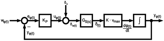
Figure 5.
Linearized variant of the orientation controller.
The controller used is a P controller with gain . The reason for this is that the system itself exhibits integral behaviour. If the pole of the controller at the origin is added to the pole of the system at the origin, there is likely no longer be a suitable controller configuration in which the control loop is stable.
Next, the pre-control generates a steering angle δV, which is added to the manipulated variable . The steering angle setpoint is denoted as δw(t). The dynamics delay the of the steering, resulting in the real steering angle δt. With the linearized variant of the single-track model, it is transformed into a change in orientation by simple amplification. The orientation results from the temporal integration of the change in orientation. Its inverse is fed back to the controller and calculated with the orientation reference value for the control error . The controller is dimensioned for the constant drive speed vmax. The constant has a value of 3.
The transfer function of the orientation control loop can now be calculated from the linear block diagram. The open loop transfer function with no feedforward is as follows:
With the dynamics of steering according to Equation (27) results in the following:
Accordingly, the closed-loop transfer function is as follows:
In the normal case, the two poles of the closed control loop can be determined from the characteristic equation.
However, because it is transcendent, it cannot be solved analytically. Therefore, the gain is sought by trial and error, where both poles are almost identical. This can be done by successively increasing and plotting the left side of Equation (32) versus at each step. For the parameters already determined, this results in critical gain as follows:
With this, the control loop begins to oscillate. Therefore, it should not be exceeded.
4.1. Constant of Proportionality
It briefly explains how to convert between them to quantities, i.e., encoder pulses (EncImp) and meters (m). The robot’s path is fixed and straight, i.e., 10,000 EncImp, with marked starting and ending points. To express the proportionality, we use
where denotes the proportionality constant. Using a ruler, the travelled distance length of 5.8 m during the test was measured. Using (34), we can record the proportionality constant as follows:
4.2. Straight Route Driving
In this section, the trajectories are evaluated. A straight driving route is examined with a focus on controlling the position and orientation. The travelled distance of the robot orientation is presented in Figure 6, while the position in the X–Y plane is given in Figure 7. It is observed from the results that the measured values are not even while the robot orientation is in a jagged position. In the laboratory test, the total covered distance was 4 m in the north–east direction with an orientation around −57°.
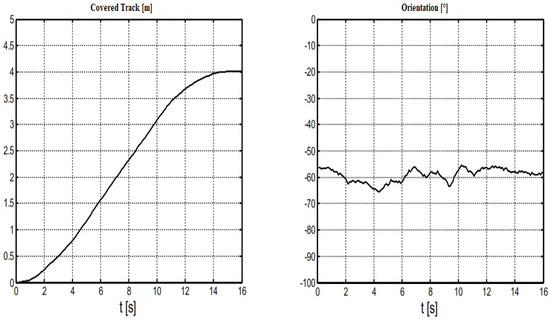
Figure 6.
Robot trajectory and orientation for straight route driving.
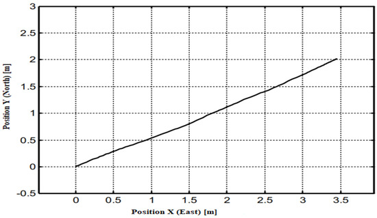
Figure 7.
Driven trajectory over the straight path.
The typical S-curve of a trapezoidal speed profile is shown in the distance travelled graph. The final destination at 4 m = 6896 EncImp is approached with full agreement. The orientation shows a small fluctuation around the target value of −57°. It is observed that the fluctuation from the target value is quite small, i.e., around 10°. The reason for small deviation is that the steering and measurement’s nonlinearity was recorded without correcting the zero point. On the other hand, the robot trajectory path was correctly recorded and is straightly driven as was estimated. This shows the optimality of the controllers in the desired values.
4.3. Turn toward Right Direction
The next task is measuring the right turn, which is recorded with an angle of 84° (−64° … −148°), and the target distance is 3 m = 5172 EncImp. This distance can be regarded as the fourth part of the circle. The distance covered by the robot orientation with the target value and the actual value is shown in Figure 8. At the same time, the driven trajectory along the X–Y plane is presented in Figure 9. The circle of motion of the robot is reconstructed with the three randomly selected trajectory points.
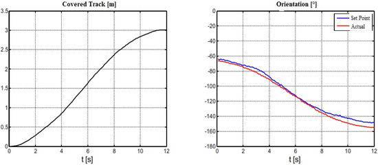
Figure 8.
Robot trajectory and orientation for turning right direction.
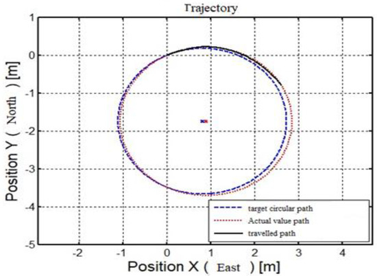
Figure 9.
Driven trajectory over the right direction.
From Figure 8, it is seen that the driven trajectory is quite straight without any disturbances. Thus, we obtained the same S-shape results as before in Figure 6; however, for the orientation, the results recorded are different from those shown in Figure 6. From Figure 8, it is seen that there is full agreement between the actual value curve and the setpoint curve.
The robot’s trajectory shown in Figure 9 is drawn by a black line, which shows the circular motion of the robot in a nice manner. The red curve is drawn from the randomly selected trajectory points, which is used to compare the two results. The results in Figure 9 show only a small deviation between the travelled path and the actual path. In this case, the controller shows a smooth working scenario.
4.4. Automatic Circular Motion
In this section, we perform an impressive test of automatic circular motion. Auto-calibration of the magnetometer [48] is carried out, then the robot is left to move twice over a circular track on the university campus.
Two tracks are shown in Figure 10, i.e., clockwise and counter-clockwise. The trajectory results are measured and superimposed using the aerial photograph from Google Maps. The trajectory size was selected to reasonably fit the building for the best measurements and retain the aspect ratio and orientation.
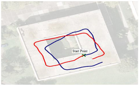
Figure 10.
Self-estimates of robot position, red (clockwise) and blue (counter-clockwise).
In Figure 10, the red trajectory (clockwise) was first measured. The calibration of the magnetometer is very smoothly conducted, as seen by the results. The starting and ending values are the same, but the image slightly differs. This happens because there is an incremental value, which adds to the first value. This control-error-accumulation value leads to an error, which results in a small deviation from the actual value. The error could be the wrong calibration of the magnetometer or other sources of interference in the building.
4.5. A Complex Route
The other test was conducted considering the complex route in the same EE building. In such a track, different tracks are considered, starting from a point, covering a distance and then returning. A distance of 10 m is considered in this track while keeping the original orientation. The values and the track are presented in Table 4.
Table 4.
Track plane with distance and orientation.
In Figure 11, three lines are drawn, represented the target value, actual path and target path. The results show agreement between the target and the actual path with a slight deviation. Multiple experiments were conducted in the healthcare system environment, e.g., patient ward, and practically evaluated the working of auto-MERLIN. These tests were performed to see the number of hits to static obstacles. To minimize the error/collisions, the robot’s orientation control was well programmed, as shown in Figure 2. The site selection was the general medicine ward of a local healthcare system. A distance of 12 m was selected between the doctor’s office and the patient’s ward. A flow diagram of the path followed by the robot using Google Maps is shown in Figure 12.
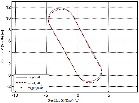
Figure 11.
Calculated and driven trajectories.
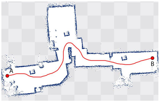
Figure 12.
Experimental verification: from doctor’s office to the patient room in a healthcare system.
The implementation of the robot in a specialized environment is an additional advantage of the proposed solution. A simulation in an environment is given below for further clearance. An open-source 3D robotics simulator called Gazebo is utilized to simulate a healthcare setting in which the robot’s maneuverability and control capabilities in various environments or scenarios are tested. The results are shown in Figure 13.
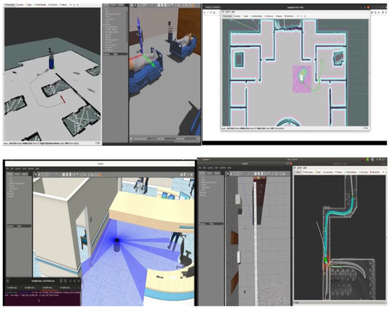
Figure 13.
Different environment simulation using Gazebo software.
5. Conclusions
In the current research work, the design of the orientation controller was proposed. For optimum maneuverability of the robot, the controller design plays a vital role, which should be analyzed. Orientation control models of the robot were also developed. In the case of the robot, the orientation and speed control design is the main objective of the proposed research. We derived and analyzed the design of the orientation controller and successfully implemented it. Various experimental tests were conducted to measure the robot’s performance, and the results were recorded. The test drive was developed by obtaining different orientation tests, including left/right turn and auto-motion over a circular and complex path.
The mini-computer program is used to control the robot remotely. In addition, sonar distance sensors and a magnetometer for determining orientation are connected. There is also a PWM output for a model-making servo motor to steer the robot. The speed of the drive is read via an incremental optical encoder. To see the robot’s behavior in the healthcare system, the robot was experimented on in the center to travel from the doctor’s office to the patient. The robot accepts target points, which it approaches independently. Various tracks are evaluated, i.e., straight, right, self-localization and complex routes. The maneuverability and control of the robot were tested, and step responses were recorded. The trajectory and orientation of the robot were measured, and good agreement between the actual and target values was recorded. From the results, it is concluded that the designed controller maintained the desired path. We designed auto-MERLIN for static obstacles to verify the proposed study and perform an experiment. The experiment shows that the robot follows the given track as desired. There are many future directions for further work on auto-MERLIN. The first task could be the robot design of dynamic obstacles. The other task could be writing software drivers for currently unused hardware. The other limitation is that the design focuses on static obstacles, while future directions can include dynamic obstacles.
Author Contributions
Conceptualization, A.A. and A.S.; methodology, M.N.K.; software, M.N.K.; validation, A.A., A.S. and M.N.K.; formal analysis, M.N.K. and M.T.; investigation, A.S. and M.T.; resources, A.S.; writing—original draft preparation, M.N.K.; writing—review and editing, A.S. and M.T.; supervision, M.N.K. and M.T.; funding acquisition, A.A. All authors have read and agreed to the published version of the manuscript.
Funding
This work was supported by the Deanship of Scientific Research at Prince Sattam bin Abdulaziz University under the research project (PSAU/2023/01/22425).
Institutional Review Board Statement
Not applicable.
Informed Consent Statement
Not applicable.
Data Availability Statement
Not applicable.
Acknowledgments
The authors acknowledge the support of the Ministry of Education in Saudi Arabia, and Faculty of Computing and Information Technology, King Abdulaziz University, Jeddah 21589, Saudi Arabia.
Conflicts of Interest
The authors declare no conflict of interest.
References
- Shahzad, A.; Roth, H. Teleoperation of mobile robot using event based controller and real time force feedback. In Proceedings of the International Workshops on Electrical and Computer Engineering Subfields, Istanbul, Turkey, 22–23 August 2014; Koc University: Istanbul, Turkey, 2014; pp. 7–12. [Google Scholar]
- Stotko, P.; Krumpen, S.; Hullin, M.B.; Weinmann, M.; Klein, R. SLAMCast: Large-scale, real-time 3D reconstruction and streaming for immersive multi-client live telepresence. IEEE Trans. Vis. Comput. Graph. 2019, 25, 2102–2112. [Google Scholar] [CrossRef]
- Gorjup, G.; Dwivedi, A.; Elangovan, N.; Liarokapis, M. An intuitive, affordances oriented telemanipulation framework for a dual robot arm hand system: On the execution of bimanual tasks. In Proceedings of the IEEE/RSJ International Conference on Intelligent Robots and Systems (IROS), Macau, China, 4–8 November 2019; IEEE: New York, NY, USA, 2019; pp. 3611–3616. [Google Scholar]
- G-Climent, S.; Garzo, A.; M-Alcaraz, M.N.; C-Adam, P.; Ruano, J.A.; Mejías-Ruiz, M.; Mayordomo-Riera, F.J. A usability study in patients with stroke using MERLIN, a robotic system based on serious games for upper limb rehabilitation in the home setting. J. Neuroeng. Rehabil. 2021, 18, 41. [Google Scholar] [CrossRef]
- Karimi, M.; Roncoli, C.; Alecsandru, C.; Papageorgiou, M. Cooperative merging control via trajectory optimization in mixed vehicular traffic. Transp. Res. Part C Emerg. Technol. 2020, 116, 102663. [Google Scholar] [CrossRef]
- Shahzad, A.; Al-jarrah, R.; Roth, H. Telecontrol of AutoMerlin robot by employing fuzzy logic. Int. J. Mech. Eng. Robot. Res. (IJMERR) 2016, 5, 17–22. [Google Scholar] [CrossRef]
- Shahzad, A.; Al-jarrah, R.; Roth, H. Teleoperation of AutoMerlin by inculcating FIN algorithm. Int. J. Mech. Eng. Robot. Res. (IJMERR) 2016, 5, 1–5. [Google Scholar] [CrossRef]
- Kitazawa, O.; Kikuchi, T.; Nakashima, M.; Tomita, Y.; Kosugi, H.; Kaneko, T. Development of power control unit for compact-class vehicle. SAE Int. J. Altern. Powertrains 2016, 5, 278–285. [Google Scholar] [CrossRef]
- Shahzad, A.; Salahudin, M.; Hussain, I. AutoMerlin mobile robot’s bilateral telecontrol with random delay. 3c Technol. 2019, 1, 179–191. [Google Scholar]
- Li, L.; Liu, Z.; Ma, Z.; Liu, X.; Yu, J.; Huang, P. Adaptive neural learning finite-time control for uncertain teleoperation system with output constraints. J. Intell. Robot. Syst. 2022, 105, 76. [Google Scholar] [CrossRef]
- R-Lera, F.J.; M-Olivera, V.; C-González, M.Á.; M-Rico, F. HiMoP: A three-component architecture to create more human-acceptable social-assistive robots. Cogn. Process. 2018, 19, 233–244. [Google Scholar] [CrossRef]
- Thomas, L.; Lueth, T.C.; Rembold, U.; Woern, H. A distributed control architecture for autonomous mobile robots-implementation of the Karlsruhe Multi-Agent Robot Architecture (KAMARA). Adv. Robot. 1997, 12, 411–431. [Google Scholar]
- Shahzad, A.; Roth, H. Bilateral telecontrol of AutoMerlin mobile robot with fix communication delay. In Proceedings of the IEEE International Conference on Automation, Quality and Testing, Robotics, Cluj-Napoca, Romania, 19–21 May 2016; IEEE: New York, NY, USA, 2016; pp. 1–6. [Google Scholar]
- Naceri, A.; Elsner, J.; Tröbinger, M.; Sadeghian, H.; Johannsmeier, L.; Voigt, F.; Chen, X.; Macari, D.; Jähne, C.; Berlet, M.; et al. Tactile robotic telemedicine for safe remote diagnostics in times of Corona: System design, feasibility and usability study. IEEE Robot. Autom. Lett. 2022, 7, 10296–10303. [Google Scholar] [CrossRef]
- de Oliveira, R.W.S.M.; Bauchspiess, R.; Porto, L.H.S.; de Brito, C.G.; Figueredo, L.F.C.; Borges, G.A.; Ramos, G.N. A robot architecture for outdoor competitions. J. Intell. Robot. Syst. 2020, 99, 629–646. [Google Scholar] [CrossRef]
- Cuesta, F.; Ollero, A.; Arrue, B.C.; Braunstingl, R. Intelligent control of nonholonomic mobile robots with fuzzy perception. Fuzzy Sets Syst. 2003, 134, 47–64. [Google Scholar]
- Ahmadzadeh, A.; Jadbabaie, A.; Kumar, V.; Pappas, G.J. Multi-UAV cooperative surveillance with spatio-temporal specifications. In Proceedings of the 45th IEEE Conference on Decision and Control, San Diego, CA, USA, 13–15 December 2006; IEEE: New York, NY, USA, 2006; pp. 5293–5298. [Google Scholar]
- Anavatti, S.G.; Francis, S.L.; Garratt, M. Path-planning modules for autonomous vehicles: Current status and challenges. In Proceedings of the International Conference on Advanced Mechatronics, Intelligent Manufacture, and Industrial Automation (ICAMIMIA), Surabaya, Indonesia, 15–17 October 2015; IEEE: New York, NY, USA, 2015; pp. 205–214. [Google Scholar]
- Kress, R.L.; Hamel, W.R.; Murray, P.; Bills, K. Control strategies for teleoperated Internet assembly. IEEE/ASME Trans. Mechatron. 2001, 6, 410–416. [Google Scholar] [CrossRef]
- Subahi, A.F.; Khalaf, O.I.; Alotaibi, Y.; Natarajan, R.; Mahadev, N.; Ramesh, T. Modified Self-Adaptive Bayesian Algorithm for Smart Heart Disease Prediction in IoT System. Sustainability 2022, 14, 14208. [Google Scholar] [CrossRef]
- Alimohammadirokni, M.; Emadlou, A.; Yuan, J.J. The strategic resources of a gastronomy creative city: The case of San Antonio, Texas. J. Gastron. Tour. 2021, 5, 237–252. [Google Scholar] [CrossRef]
- Singh, S.P.; Alotaibi, Y.; Kumar, G.; Rawat, S.S. Intelligent Adaptive Optimisation Method for Enhancement of Information Security in IoT-Enabled Environments. Sustainability 2022, 14, 13635. [Google Scholar] [CrossRef]
- Nagappan, K.; Rajendran, S.; Alotaibi, Y. Trust Aware Multi-Objective Metaheuristic Optimization Based Secure Route Planning Technique for Cluster Based IIoT Environment. IEEE Access 2022, 10, 112686–112694. [Google Scholar] [CrossRef]
- Alotaibi, Y.; Noman Malik, M.; Hayat Khan, H.; Batool, A.; ul Islam, S.; Alsufyani, A.; Alghamdi, S. Suggestion Mining from Opinionated Text of Big Social Media Data. Comput. Mater. Contin. 2021, 68, 3323–3338. [Google Scholar] [CrossRef]
- Kebria, P.M.; Khosravi, A.; Nahavandi, S.; Shi, P.; Alizadehsani, R. Robust Adaptive Control Scheme for Teleoperation Systems With Delay and Uncertainties. IEEE Trans. Cybern. 2020, 50, 3243–3253. [Google Scholar] [CrossRef]
- Lakshmanna, K.; Subramani, N.; Alotaibi, Y.; Alghamdi, S.; Khalafand, O.I.; Nanda, A.K. Improved Metaheuristic-Driven Energy-Aware Cluster-Based Routing Scheme for IoT-Assisted Wireless Sensor Networks. Sustainability 2022, 14, 7712. [Google Scholar] [CrossRef]
- Anuradha, D.; Subramani, N.; Khalaf, O.I.; Alotaibi, Y.; Alghamdi, S.; Rajagopal, M. Chaotic Search-and-Rescue-Optimization-Based Multi-Hop Data Transmission Protocol for Underwater Wireless Sensor Networks. Sensors 2022, 22, 2867. [Google Scholar] [CrossRef]
- Tirandazi, P.; Rahiminasab, A.; Ebadi, M.J. An efficient coverage and connectivity algorithm based on mobile robots for wireless sensor networks. J. Ambient. Intell. Humaniz. Comput. 2022, 1–23. [Google Scholar] [CrossRef]
- Sennan, S.; Kirubasri; Alotaibi, Y.; Pandey, D.; Alghamdi, S. EACR-LEACH: Energy-Aware Cluster-based Routing Protocol for WSN Based IoT. Comput. Mater. Contin. 2022, 72, 2159–2174. [Google Scholar] [CrossRef]
- Rozevink, S.G.; van der Sluis, C.K.; Garzo, A.; Keller, T.; Hijmans, J.M. HoMEcare aRm rehabiLItatioN (MERLIN): Telerehabilitation using an unactuated device based on serious games improves the upper limb function in chronic stroke. J. Neuroeng. Rehabilitation 2021, 18, 48. [Google Scholar] [CrossRef]
- Schilling, K. TELE-MAINTENANCE OF INDUSTRIAL TRANSPORT ROBOTS. IFAC Proc. Vol. 2002, 35, 139–142. [Google Scholar] [CrossRef]
- Shahzad, A.; Roth, H. Bilateral telecontrol of AutoMerlin mobile robot. In Proceedings of the 9th IEEE International Conference on Open-Source Systems and Technologies, Lahore, Pakistan, 17–19 December 2015; IEEE: New York, NY, USA, 2015; pp. 179–191. [Google Scholar]
- Zhang, W.; Cheng, H.; Zhao, L.; Hao, L.; Tao, M.; Xiang, C. A Gesture-Based Teleoperation System for Compliant Robot Motion. Appl. Sci. 2019, 9, 5290. [Google Scholar] [CrossRef]
- Su, Y.-P.; Chen, X.-Q.; Zhou, T.; Pretty, C.; Chase, G. Mixed-Reality-Enhanced Human–Robot Interaction with an Imitation-Based Mapping Approach for Intuitive Teleoperation of a Robotic Arm-Hand System. Appl. Sci. 2022, 12, 4740. [Google Scholar] [CrossRef]
- Ahmad, A.; Babar, M.A. Software architectures for robotic systems: A systematic mapping study. J. Syst. Softw. 2016, 122, 16–39. [Google Scholar] [CrossRef]
- Sharma, O.; Sahoo, N.; Puhan, N. Recent advances in motion and behavior planning techniques for software architecture of autonomous vehicles: A state-of-the-art survey. Eng. Appl. Artif. Intell. 2021, 101, 104211. [Google Scholar] [CrossRef]
- Ziegler, J.; Werling, M.; Schroder, J. Navigating car-like robots in unstructured environments using an obstacle sensitive cost function. In Proceedings of the IEEE Intelligent Vehicles Symposium, Eindhoven, The Netherlands, 4–6 June 2008; IEEE: New York, NY, USA, 2008; pp. 787–791. [Google Scholar]
- G-Santamarta, M.A.; R-Lera, F.J.; A-Aparicio, C.; G-Higueras, A.M.; F-Llamas, C. MERLIN a cognitive architecture for service robots. Appl. Sci. 2020, 10, 5989. [Google Scholar] [CrossRef]
- Shao, J.; Xie, G.; Yu, J.; Wang, L. Leader-following formation control of multiple mobile robots. In Proceedings of the IEEE International Symposium on, Mediterrean Conference on Control and Automation Intelligent Control, Limassol, Cyprus, 27–29 June 2015; IEEE: New York, NY, USA, 2005; pp. 808–813. [Google Scholar]
- Faisal, M.; Hedjar, R.; Al Sulaiman, M.; Al-Mutib, K. Fuzzy Logic Navigation and Obstacle Avoidance by a Mobile Robot in an Unknown Dynamic Environment. Int. J. Adv. Robot. Syst. 2013, 10, 37. [Google Scholar] [CrossRef]
- Favarò, F.; Eurich, S.; Nader, N. Autonomous vehicles’ disengagements: Trends, triggers, and regulatory limitations. Accid. Anal. Prev. 2018, 110, 136–148. [Google Scholar] [CrossRef]
- Gopalswamy, S.; Rathinam, S. Infrastructure enabled autonomy: A distributed intelligence architecture for autonomous vehicles. In Proceedings of the IEEE Intelligent Vehicles Symposium (IV), Changshu, China, 26–30 June 2018; IEEE: New York, NY, USA, 2018; pp. 986–992. [Google Scholar]
- Allen, J.F. Towards a general theory of action and time. Artif. Intell. 1984, 23, 123–154. [Google Scholar] [CrossRef]
- Hu, H.; Brady, J.M.; Grothusen, J.; Li, F.; Probert, P.J. LICAs: A modular architecture for intelligent control of mobile robots. In Proceedings of the IEEE/RSJ International Conference on Intelligent Robots and Systems. Human Robot Interaction and Cooperative Robots, Pittsburgh, PA, USA, 5–9 August 1995; IEEE: New York, NY, USA, 1995; pp. 471–476. [Google Scholar]
- Zhao, W.; Gao, Y.; Ji, T.; Wan, X.; Ye, F.; Bai, G. Deep Temporal Convolutional Networks for Short-Term Traffic Flow Forecasting. IEEE Access 2019, 7, 114496–114507. [Google Scholar] [CrossRef]
- Schilling, K.J.; Vernet, M.P. Remotely controlled experiments with mobile robots. In Proceedings of the 34th IEEE Southeastern Symposium on System Theory, Huntsville, AL, USA, 17–19 March 2002; IEEE: New York, NY, USA, 2002; pp. 71–74. [Google Scholar]
- Lefèvre, S.; Vasquez, D.; Laugier, C. A survey on motion prediction and risk assessment for intelligent vehicles. ROBOMECH J. 2014, 1, 1. [Google Scholar] [CrossRef]
- Behere, S.; Törngren, M. A functional reference architecture for autonomous driving. Inf. Softw. Technol. 2016, 73, 136–150. [Google Scholar] [CrossRef]
- Carvalho, A.; Lefévre, S.; Schildbach, G.; Kong, J.; Borrelli, F. Automated driving: The role of forecasts and uncertainty—A control perspective. Eur. J. Control. 2015, 24, 14–32. [Google Scholar] [CrossRef]
- Weiskircher, T.; Wang, Q.; Ayalew, B. Predictive Guidance and Control Framework for (Semi-)Autonomous Vehicles in Public Traffic. IEEE Trans. Control. Syst. Technol. 2017, 25, 2034–2046. [Google Scholar] [CrossRef]
- Li, R.; Wang, H.; Liu, Z. Survey on Mapping Human Hand Motion to Robotic Hands for Teleoperation. IEEE Trans. Circuits Syst. Video Technol. 2021, 32, 2647–2665. [Google Scholar] [CrossRef]
- Muscolo, G.G.; Marcheschi, S.; Fontana, M.; Bergamasco, M. Dynamics Modeling of Human–Machine Control Interface for Underwater Teleoperation. Robotica 2021, 39, 618–632. [Google Scholar] [CrossRef]
- Ogunrinde, I.O.; Adetu, C.F.; Moore, C.A.; Roberts, R.G.; McQueen, K. Experimental Testing of Bandstop Wave Filter to Mitigate Wave Reflections in Bilateral Teleoperation. Robotics 2020, 9, 24. [Google Scholar] [CrossRef]
- Liu, Q.; Chen, H.; Wang, Z.; He, Q.; Chen, L.; Li, W.; Li, R.; Cui, W. A Manta Ray Robot with Soft Material Based Flapping Wing. J. Mar. Sci. Eng. 2022, 10, 962. [Google Scholar] [CrossRef]
- Li, W.K.; Chen, H.; Cui, W.C.; Song, C.H.; Chen, L.K. Multi-objective evolutionary design of central pattern generator network for biomimetic robotic fish. Complex Intell. Syst. 2022, 9, 1707–1727. [Google Scholar] [CrossRef]
- Riekert, P.; Schunck, T.-E. Zur fahrmechanik des gummibereiften kraftfahrzeugs. Ing.-Arch. 1940, 11, 210–224. [Google Scholar] [CrossRef]
Disclaimer/Publisher’s Note: The statements, opinions and data contained in all publications are solely those of the individual author(s) and contributor(s) and not of MDPI and/or the editor(s). MDPI and/or the editor(s) disclaim responsibility for any injury to people or property resulting from any ideas, methods, instructions or products referred to in the content. |
© 2023 by the authors. Licensee MDPI, Basel, Switzerland. This article is an open access article distributed under the terms and conditions of the Creative Commons Attribution (CC BY) license (https://creativecommons.org/licenses/by/4.0/).