Featured Application
Audio classification; music information retrieval; audio scene characterization; temporal localization of sound sources; audio indexing; audio surveillance systems; anomaly detection from audio sounds.
Abstract
Sound event detection (SED) is the task of finding the identities of sound events, as well as their onset and offset timings from audio recordings. When complete timing information is not available in the training data, but only the event identities are known, SED should be solved by weakly supervised learning. The conventional U-Net with global weighted rank pooling (GWRP) has shown a decent performance, but extensive computation is demanded. We propose a novel U-Net with limited upsampling (LUU-Net) and global threshold average pooling (GTAP) to reduce the model size, as well as the computational overhead. The expansion along the frequency axis in the U-Net decoder was minimized, so that the output map sizes were reduced by 40% at the convolutional layers and 12.5% at the fully connected layers without SED performance degradation. The experimental results on a mixed dataset of DCASE 2018 Tasks 1 and 2 showed that our limited upsampling U-Net (LUU-Net) with GTAP was about 23% faster in training and achieved 0.644 in audio tagging and 0.531 in weakly supervised SED tasks in terms of F1 scores, while U-Net with GWRP showed 0.629 and 0.492, respectively. The major contribution of the proposed LUU-Net is the reduction in the computation time with the SED performance being maintained or improved. The other proposed method, GTAP, further improved the training time reduction and provides versatility for various audio mixing conditions by adjusting a single hyperparameter.
1. Introduction
The purpose of sound event detection (SED) is figuring out the types of sound sources contained in the input audio recordings. SED can be used in a surveillance system that detects the occurrence of a specific sound [1,2], voice activity detection (VAD) [3], or keyword spotting with the human voice [4]. Currently, SED systems are usually implemented by convolutional neural networks (CNNs) [5,6], recurrent neural networks (RNNs) [2], or combinations of them [7,8,9]. SED solutions early on usually relied on a supervised learning framework that required a completely labeled dataset [10] in which the onset and offset timings of the sound events were transcribed. However, complete labeling of all the timings would require too much effort from human listeners, and often, they are not available in practical situations. In more realistic cases, only the types of sound events of the audio recordings are known, as shown in Figure 1. Strong labels include onset and offset times in the given audio recordings, but weak labels give only the types of audio events. When incomplete information is given, the task is called weakly supervised classification [11,12,13,14,15,16,17]. Using weakly supervised learning with an incompletely labeled dataset might reduce the costs for dataset construction. One of the weakly supervised classifications is generating a strongly labeled dataset from the given weakly supervised training data [16]. This framework generates strongly labeled sound event timings by clipping sound event audio, normalizing it, and then synthesizing it with normalized background audio or white noise. This is similar to data augmentation, but with this framework, it is possible to increase the quantity of the dataset. In addition, natural environments are polyphonic, meaning that multiple sounds may be active at the same time [1,2,17]. Therefore, the sound event occurrences overlap. There are no predefined rules on how sounds can co-occur, and the way to model co-occurrence is through random sampling with the degree of overlap of different classes given by or obtained from the data statistics. To detect polyphonic sound events, multi-label classifiers are required [1].

Figure 1.
Examples of strong and weak labels. A strong label consists of a sequence of sound event types and onset and offset times in the given recording. A weak label consists of sound event types only.
The SED model is usually based on weakly supervised CNNs [16,17,18]. When training CNNs, only the event labels are used as targets. In the detection stage, video object description models (VODMs) such as cascade R-CNN (regions with CNN features) [19], faster R-CNN [20], and the class activation map (CAM) approach [21] are used. The 2D object regions or class activation maps obtained by a trained CNN are used to predict the onset and offset times of the classified audio events. Another type of SED approach is using temporal models such as convolutional recurrent neural networks (CRNNs) [1,22] and Transformers [23]. These temporal models are able to find the onset and offset timings more accurately because they are inferred simultaneously with the class labels in a single learning stage. The aforementioned weakly supervised learning methods require generating onset and offset timings that are obtained in an unsupervised manner, so the accuracy of the detection varies greatly according to the types of audio sources and the characteristics of the recording environments. Self-supervised learning [24] and pseudo-labeling [25] methods for weakly supervised SED have been proposed, but their performances rely on specific audio events only. Recently, U-Net showed successful performance in image segmentation and also was applied to SED [16,26]. U-Net was originally designed for segmentation tasks, so in a weakly supervised manner, the segmentation targets are converted to sound event category labels by global pooling techniques such as global average pooling (GAP) [27,28], global max pooling (GMP) [16], and global weighted rank pooling (GWRP) [18]. However, these methods require averaging or sorting operations on the total feature map, so their is an extensive computational overhead.
In this paper, we propose two kinds of methods that can improve the performance of the weakly supervised SED, as well as reduce the time and space complexity. The proposed model is a modification of the U-Net structure [16,26] suited for sound event detection. The first method is a limited upsampling from the lower layers to the higher ones in the decoder part of U-Net. Because SED performs temporal segmentation only, we did not apply upsampling along the frequency axis in the U-Net decoder, and thus, the output map sizes were reduced greatly without performance loss. According to the experimental results, a total of 40% of the convolution output map size and 12.5% of the fully connected layer output were required to provide slightly better SED performance. The second proposed method is a global pooling technique called global threshold average pooling (GTAP). The conventional GWRP requires sorting the total output map, and its time complexity grows with the growth of the output map size. The proposed method uses a fixed threshold to determine the set of the output map units for the average pooling. The threshold computation requires the mean and the standard deviation of the map values, which is much faster than the sorting operation. Moreover, higher SED performance can be obtained by adjusting the threshold with a single hyperparameter. The major contribution of the proposed methods is the reduction of the computation time without any performance loss. The size of the bottleneck layer of U-Net is the same for the proposed LUU-Net, so the amount of information for the audio events transferred to the final output is the same. The proposed LUU-Net limits the expansion along the frequency axis only, and the time resolution in the time domain is kept unchanged. While doing so, the network size of the encoder is reduced by up to , resulting in a 40% reduction in the number of parameters. The proposed GTAP further improves the computation time by pruning unnecessary output map components, with the SED and AT performances being improved over the conventional CNN and U-Net.
The rest of this paper is organized as follows. Section 2 describes the conventional SED method based on U-Net and GWRP. Section 3 explains the proposed U-Net with limited upsampling and the proposed global threshold average pooling (GTAP). Section 4 gives the experiments’ setup and the results with a detailed analysis. Finally, Section 6 summarizes our contribution.
2. Conventional Sound Event Detection
In this section, we explain the sound event detection problem in detail and the conventional methods for the problem.
2.1. Weakly Supervised Sound Event Detection Framework
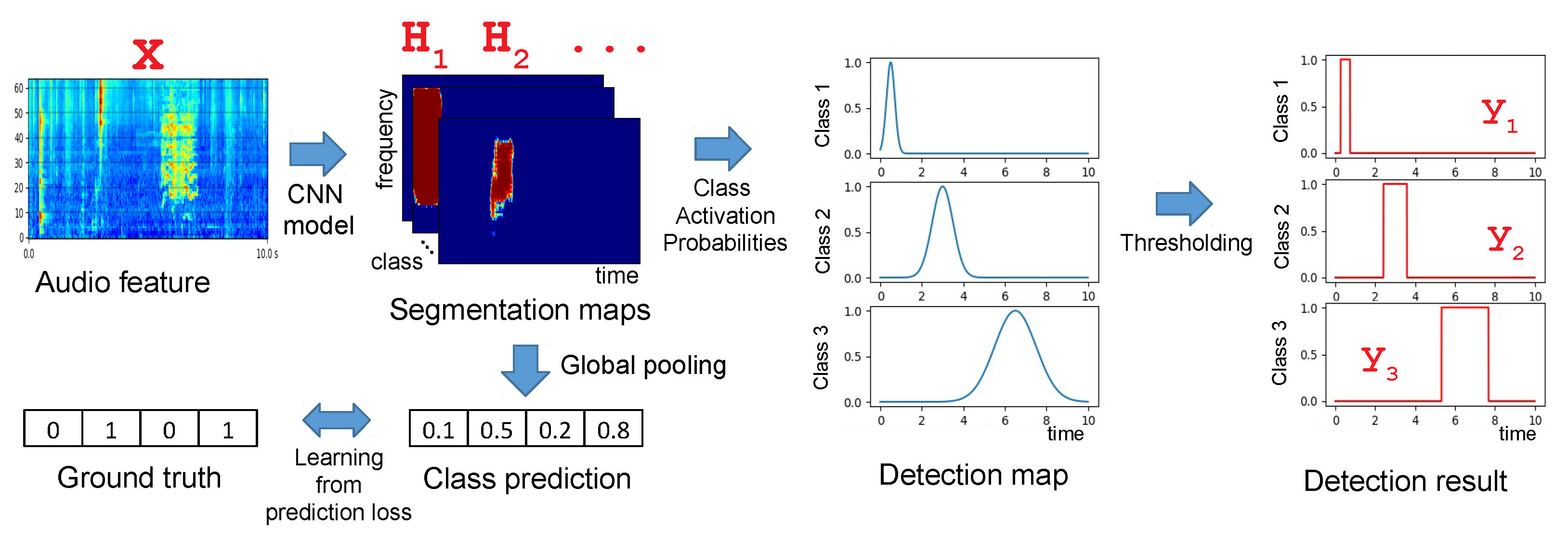
Figure 2 shows the basic architecture of the weakly supervised learning framework for sound event detection. The input audio features are passed through a number of convolution layers to generate segmentation maps in 1D or 2D space. There are two outputs for audio tagging and sound event detection, respectively. In audio tagging, true labels are given for audio class indices, so a pooling is applied to convert the segmentation maps to probabilistic predictions, and the loss is computed with respect to the given true labels. In sound event detection, the output is interpreted as a segmentation map in 1D or 2D space. Because the onset and lengths of the sound events are not given in the training dataset, sound event timings cannot be the direct training targets. The audio tagging information—the class labels of the audio events—are used to infer the sound events. A convolutional neural network (CNN) model has been proposed for the weakly supervised learning [16]. It resembles the conventional VGG network [29] with modifications. In order to ensure for the output of the model is the same size as the input of the model, there are no downsampling layers such as max or average pooling, but only nine convolutional layers. However, this makes the receptive field smaller and computational cost very expensive.

Figure 2.
Weakly supervised sound event detection framework. The outputs of convolutional layers are segmentation maps and interpreted as audio tagging and sound event detection results. Because no ground truth for detection is provided, detection loss is not used in training the network. Only classification loss is computed.
2.2. U-Net for Sound Event Detection
We first describe the weakly supervised U-Net [26] for the sound event detection (SED) task. U-Net was proposed for medical image segmentation and has shown good performance in image segmentation tasks in various fields. This model has a convolutional encoder–decoder structure and shows high reconstruction performance thanks to the skip connection between the encoder and decoder. We decided to use this model because this kind of structure is good at solving the problem of the baseline model, and then, we used this model to implement a system that trains the SED task in a weakly supervised manner.
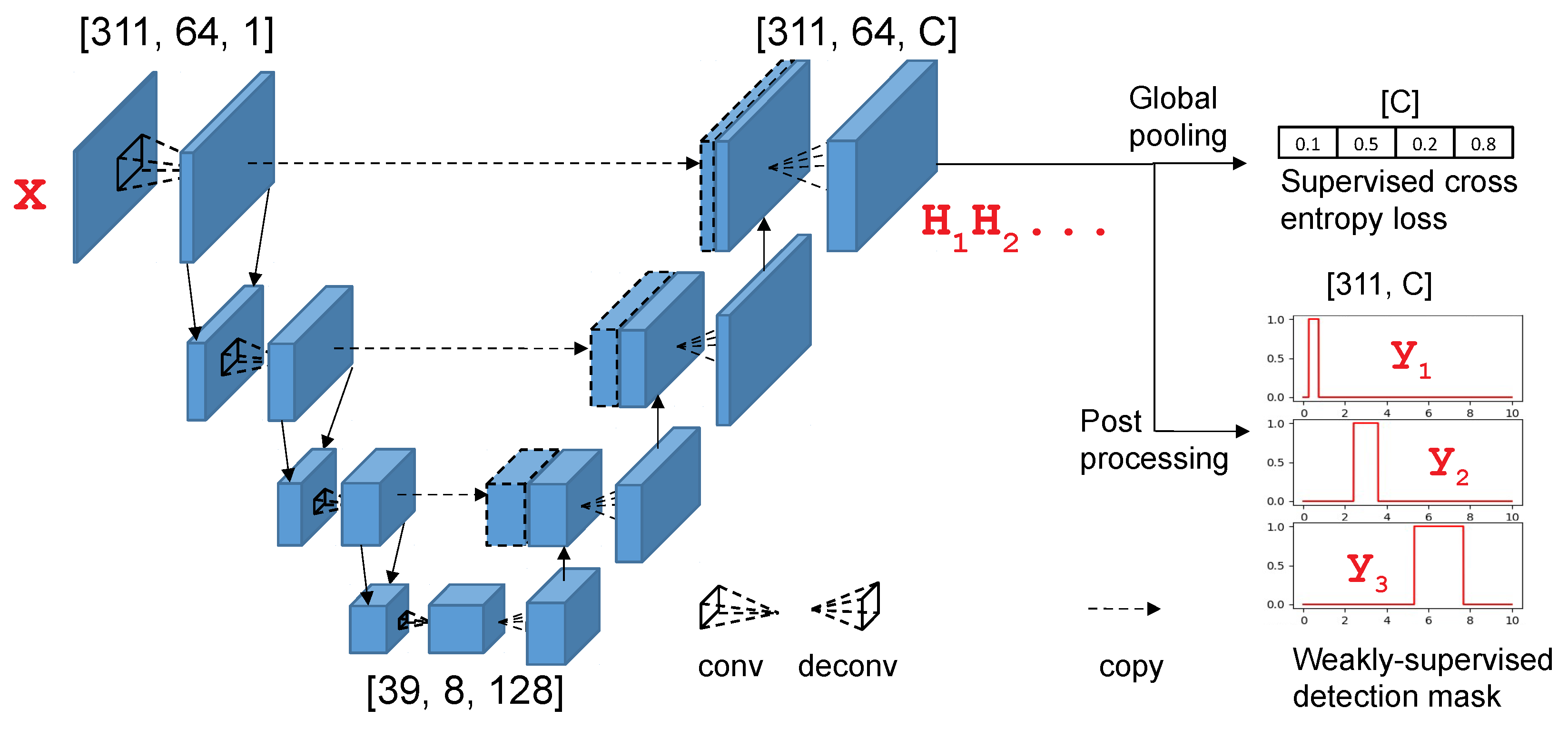
Figure 3 illustrates the U-Net architecture for the sound event detection model. In the left, the encoder part, a number of convolutional and pooling layers are repeatedly applied to reduce the input size from to , with appropriate selections of the number of convolutional kernels. In the right, the decoder part, deconvolution is applied to restore the input size, , so that the final segmentation masks are of the same size as the input spectrogram. Note that the number of masks equals the number of classes. The category predictions are obtained by global pooling and used in computing the classification loss, and the detection results are obtained by averaging the frequency components. We used supervised cross-entropy loss to train the whole network [30], which is suitable for classification tasks with their targets expressed by a one-hot representation [31].
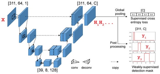
Figure 3.
U-Net architecture for weakly supervised sound event detection with full upsampling in the deconvolutional layers. The left encoder part reduces the input size to a smaller size with a number of convolutional and pooling layers. The right half, the decoder part, restores the bottom output map of a reduced size to the original input size. The number of channels at the final output layer is the same as the number of classes (a positive integer “C” in this example). For each output channel, a global pooling layer is applied to derive the audio tagging outputs, so that the number of target nodes is the same as the number of tagging classes.
The final output of the conventional U-Net [26] is a event segmentation map of the detected classes with the same dimension as the input. Training U-Nets requires a true segmentation map, to minimize the amount mismatch between the predicted segmentation result and the ground truth for each sample. When the complete ground truth map is not available, but only the class labels that exist in the input sound are given, the connection from the segmentation layer of U-Net to the class label output layer is added. The size of the segmentation map is much larger than the number of classes, so we applied GWRP [18] to reduce the map size. The resultant dimension of the GWRP output is [batch_size, number_of_classes], so that audio tagging in time domain can be achieved in a supervised manner.
2.3. Postprocessing
Figure 4 shows the detailed postprocessing procedures. The output size should become , where C is the number of event classes, as shown by the two-dimensional image in the bottom right part of Figure 3. Global pooling is performed to compute the prediction vector, whose dimension is the same as the number of classes. The prediction vector is then compared with the ground truth vector, and the prediction loss is used to train the model. In the three graphs at the bottom right of Figure 3, the y-axis is the class labels of the various sounds, and the x-axis represents the onset and the length of the sound events. This task is called audio tagging. The other task is sound event detection. The 2D classwise segmentation maps are then converted to class activation probabilities along the time axis (detection map), and simple thresholding yields the detection results, so the onset and offset times of the sound events are obtained. In sound event detection, the conversion of the 2D segmentation map to the 1D temporal detection map is the key issue. There are a number of global pooling methods for effective and efficient conversion.

Figure 4.
Postprocessing procedures for audio tagging and sound event detection. The spectro-temporal 2D audio feature map, denoted by , is converted to the 2D segmentation map of the same size () and 1D class prediction vector of length C (the number of event classes) to compute the prediction loss for audio tagging and model training. The segmentation maps are converted to C detection maps of length T (time), and thresholding is performed to find the onset and offset of the sound events ().
2.4. Global Pooling
To make predictions for audio tagging, the 2D segmentation map is compressed to a scalar value, which is generally interpreted as a probability value of the occurrence of a specific event in the input recording. The occurrences do not have to be mutually exclusive, so each segmentation map is handled independently. Global max pooling (GMP) [27] is defined as follows:
where is the segmentation map for class c and t and f are the indices of the time and frequency axes, respectively. The drawback of GMP is that it is sensitive to outliers and more affected as the segmentation map size increases. To overcome this problem, global average pooling (GAP) [27,28] provides much more stable prediction results, which is computed as
The GAP is less sensitive to outliers, but when an event occurs sparsely, the activation of the event becomes too small to be detected as having occurred. One of the efficient pooling methods that balances outlier robustness and the sparsity problem is global weighted rank pooling (GWRP) [18]. This GWRP operation is defined as follows:
where the function “” sorts the 2D input in descending order to generate a 1D sorted list of the whole elements, so is the largest value in with 2D values flattened to a 1D vector . A hyperparameter is a decaying weight enabling small activations to contributed less to the computation of the pooling output. This is a generalized weighted pooling, which is equal to GAP for d = 1 and GMP for d = 0. GWRP is good for a weakly supervised SED task because GAP overestimates and GMP underestimates the tagging result [16]. However, GWRP also has a drawback that the computation speed is very slow because the sorting must be preceded by the calculation of the weight, and it is hard to find the proper hyperparameter d.
3. Proposed Method
In this section, we describe a combination of two proposed methods for sound event detection. The first one is a novel U-Net architecture and a pooling method to improve the computational efficiency compared to the conventional U-Net. The second method uses a subset of feature maps from U-Net without sorting, denoted as global threshold average pooling (GTAP).
3.1. U-Net with Limited Upsampling
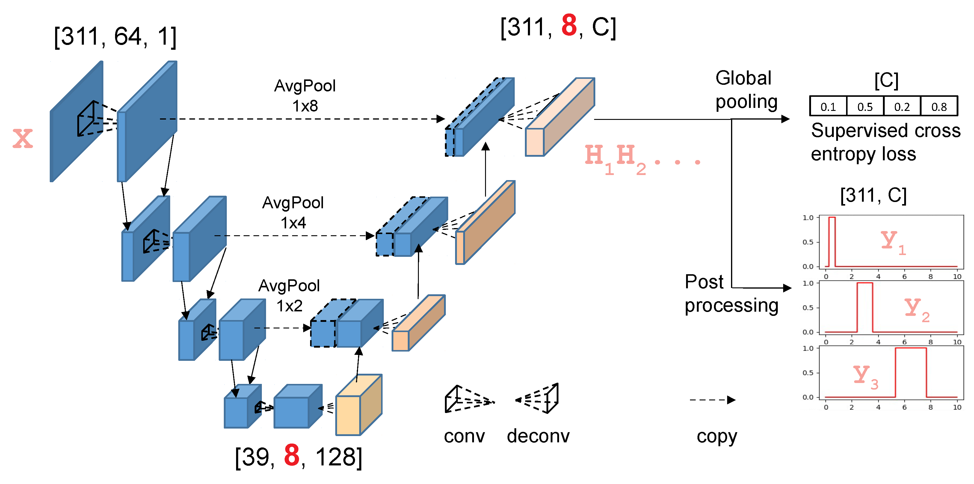
Figure 5 describes the proposed U-Net architecture with limited upsampling. Even though the segmentation map is not learned by direct loss minimization, its prediction can be obtained while minimizing the classification loss of each time frame. The U-Net-based architecture learns to generate an activation map of each event in the time–frequency domain. However, some events that activate only a few parts of the frequency bins could be ignored after postprocessing because of the average pooling. To handle this problem, reducing the frequency axis to 1 inside the model is not a good way since it removes too much representation in the middle of the model. Therefore, we further applied limited upscaling along the frequency axis in the decoder part of U-Net to keep high activation in the encoded feature. More specifically, the baseline U-Net in Figure 3 uses deconvolution with stride for upscaling in the decoder. However, the proposed U-Net uses deconvolution with stride . Therefore, compared with the existing U-Net, the size of the decoder’s feature map is smaller, which reduces the computational cost. In addition, the size of data transmitted in the skip connection between the encoder and decoder is different from the feature of the decoder. To adjust this, we downscaled the data size by using average pooling with .
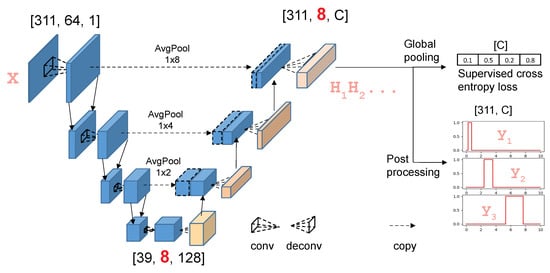
Figure 5.
U-Net architecture with limited upsampling in the deconvolutional layers. The left encoder part is the same as U-Net, but in the right, the decoder part, it only upsamples along the time axis to match the input time range.
The encoder part is unchanged, but the decoder upsamples only the time axis of the encoded features. In the example shown in Figure 5, the frequency range shrinks from 64 to 8, and the shrink size 8 is maintained in the final segmentation map. The time range changes from 311 to 39, and it goes back to 311 to restore the original time range. Upsampling in the deconvolutional layers is often unreliable because the information of the input is lost by the U-Net encoder and should be regenerated, resulting in a great amount of generation errors at the output. In a weakly supervised manner, the target information is incomplete, so more uncertainty is likely to propagate through the network, especially in the training steps. As a result, this structure reduces the size of the feature handled by the decoder, further increasing the computational efficiency. If the upscaling of the frequency axis actually interferes with learning in a weakly supervised manner, removing unnecessary upscaling may yield higher detection performance.
By comparing the U-Net in Figure 3 and the proposed LUU-Net in Figure 5, the size of the bottleneck layer between the encoder and decoder networks is , and it is the same for both models. The information transferred from the input to the output through the network is the same. In U-Net, the deconvolutional layers in the decoder part restore the original frequency and time axes to obtain the segmentation masks in the frequency and time domain. However, SED does not require the segmentation mask in the frequency domain. The proposed LUU-Net expands the time axis only, and the segmentation mask can be obtained more reliably by removing unnecessary expansion from the bottleneck layers with the same amount of information. Therefore, LUU-Net is more efficient than U-Net in SED tasks without loss of information.
3.2. Global Threshold Average Pooling
The GWRP in Section 2.4 requires a sorted list of whole segmentation map elements. The sorting is required both in training and testing, so there is a large computational overhead. Moreover, the hyperparameter d is adjusted by the amount of events occurring in the map. In Equation (3), decreases as i increases because , and the value of d should be relatively large if the sound event occurs densely or the length of the event is long and small if it occurs sparsely or its length is short. When long and short events are mixed in the input recording, which is usual in real situations, it is very hard to determine a single value of d to guarantee the detection performance. Global max pooling is not influenced by the event lengths; however, it is sensitive to the outliers, and most of the segmentation map values, except the maximum, are discarded, so learning through error backpropagation may not work well.
To overcome the problems of GWRP, computational overhead, and hyperparameter adjustment, we propose a novel global pooling using a learnable threshold value. To begin with, we define the following threshold function, which is similar to the standard step function:
where m is the input and is a given threshold value. The key idea of the proposed method is averaging only the values larger than the threshold. We define global threshold average pooling (GTAP) as follows:
where is the -element of the 2D segmentation map for class c, , defined in Equation (1). is a conditional expectation, so the GTAP function is the average of the values larger than threshold . In the actual implementation, we used the following equivalent equation for more efficient calculation.
where “ReLU” is the rectified linear unit commonly used in deep neural networks.
The threshold is also relevant to the frequency and the length of the events. With the assumption that the segmentation map is distributed by a Gaussian, the appropriate threshold value is found by
where “” and “” are the mean and the standard deviation of the segmentation map and is a hyperparameter to define how tightly to cut off the segmentation map. Because it is hard to use a class-specific threshold, we used all the training data to compute the mean and the standard variation. If , the threshold value becomes smaller, which results in overestimation over . If , the threshold increases and the trained model may underestimate. A grid search is used to determine the appropriate value of using a validation set. The detailed procedure is explained in the Experiments Section.
4. Experiments
We used DCASE 2018 Task 1 and Task 2 data [32,33] to create a mixed dataset of 8000 audio samples. The original sampling rates of the DCASE dataset are 48 kHz and 44.1 kHz, and we downsampled all the data to 32 kHz. The mixed dataset was created by adding the audio recordings of Task 1 and background sounds at 0 dB and adding other audio clips of various lengths for the simulated sound events.
4.1. Dataset Generation
According to the data augmentation in previous work [16], we built a large SED training dataset from audio tagging samples by synthesizing several audio clips with white noise or other types of audio sounds as background noise sounds. This framework is regarded as one of the data augmentation methods, allowing the generation of the training dataset with the various choices of different sounds. When adding a number of different sounds, their onset times and clipping lengths are varied to simulate various overlapping cases in real situations. Figure 6 shows the procedures of training data generation. The audio sounds are represented by 2D time–frequency spectrograms. There are many combinations of onset times and clipping lengths and how much audio is in a single recording. These combinations help the trained model work well with various SED tasks.
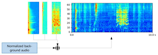
Figure 6.
Training data generation procedure. Two audio samples are mixed with a background sound. Audio samples are clipped to a given length, normalized, and then mixed with normalized background noise. The x-axis is time in seconds, and for the y-axis frequency bin index, the larger the higher it is.
Audio classification experiments were carried out on 2 different datasets to evaluate the proposed method. DCASE 2018 Task 1 is a dataset consisting of a total of 8640 audio samples [32]. Each of them is 10 s long and sampled at 48 kHz. We used it as background sounds in evaluation data synthesis. The DCASE 2018 Task 2 is an audio tagging task [33]. The tagging dataset consists of about 9500 training samples of 41 categories, which are distributed unequally and sampled at 44.1 kHz. The smallest category has 94 samples and the largest 300 samples.
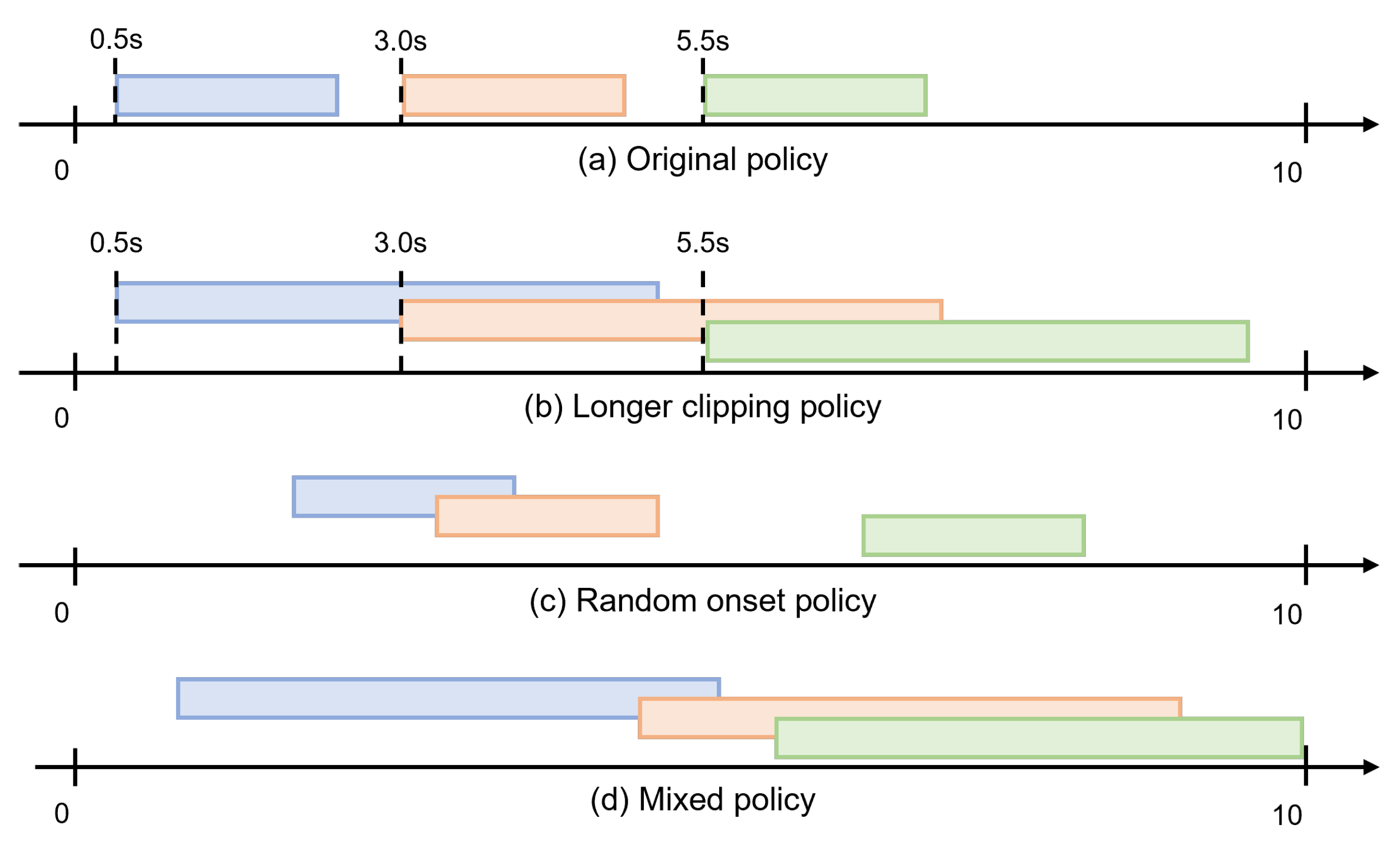
We adopted the policy suggested by the DCASE Challenge Guidelines [16] to generate the training dataset. In the original policy suggested by the DCASE Challenge, 3 distinct audio files were chosen from DCASE Task 2, clipped up to 2 s, and combined with additional background sounds to generate samples for training. The onset times were 0.5 s, 3 s, and 5.5 s, so there was no overlap among the 3 sound events. Besides the original policy, we performed several different synthetic polices: random onset, longer clipping, and mixed policies. Figure 7 shows the generated sample according to each policy. The longer clipping policy uses the maximum clip length of 5 s, which is longer than the 2 s suggested by the original guideline. This policy has a high probability of generating a sample containing overlapping events. In the random onset policy, the onsets of the events are randomly chosen from . This policy has a smaller probability of generating a sample containing overlapping events than the longer clipping policy, but in this sample, events can start at any time. The mixed policy uses both the random onset and longer clipping, making the generated sample very unpredictable. These policies are summarized in Table 1.
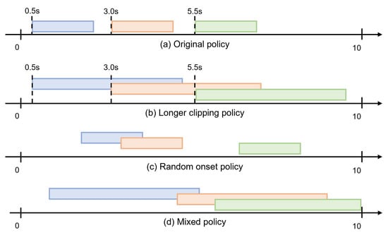
Figure 7.
Comparison of temporal overlaps of different mixing polices. (a) Original policy with no overlap; (b) longer clipping policy allowing some overlaps between events by using longer clips; (c) random onset policy allowing events to start at any time; some samples overlap, but some other samples do not due to the randomness; (d) mixed policies in (b,c). Most overlaps are observed.

Table 1.
Audio synthetic polices. All numbers are in seconds. The column names mean: onset times are the beginning of the events; max clip is the maximum clipping length; mean and std are the average and standard deviation of the clipping lengths. The row names: original is the policy suggested by the DCASE Challenge; longer clipping uses a longer maximum clipping length; random onset is varying the onset times randomly; mixed is the mixed policy of random onset and longer clipping.
4.2. Model Configurations
We compared the proposed U-Net model with the basic CNN and conventional U-Net in terms of SED performances. The basic building blocks of the models are listed in Table 2 and Table 3. We generally stacked convolutional layers () and used convolutions ()) to resize the number of output maps if necessary. One deconvolutional layer, denoted by , has stride , and is used to uncompress the x- and y-axes by a factor of 2. Another deconvolutional layer has stride and uncompresses the x-axis only, so it doubles the output map size along the time axis, but not along the frequency axis. was adopted in the proposed method only. In all the convolutional layer types, the number of output channels is given by a parameter K, and the number of inputs is determined automatically according to the previous output layers. At all the outputs of the convolutional and deconvolutional layers, we performed batch normalization and applied the rectified linear unit activation function (BN-ReLU) [34,35], as shown in Table 2. Two types of average pooling layers are used. In Table 3, uses a pooling window with the same stride size in both the time and frequency axes, so the size of the output map is reduced to half of the original in both axes. uses a pooling window with moving s samples along the time axis and 1 bin along the frequency axis, so the size of the output map decreases along the time axis only.

Table 2.
Basic convolutional blocks used in SED model construction. There are two types of convolutional layers, and , with and kernel sizes, respectively. There are also two types of deconvolutional layers. and have strides and , respectively. BN-ReLU is batch normalization and rectified linear unit activation at the output.

Table 3.
Pooling blocks and dropout layer used in SED model construction. The layer reduces the sizes by half in both the x- and y-axes, but reduces the y-axis by a factor of f, resizing the frequency axis, but not the time axis. is usually added after a convolutional layer, and is used in concatenating the output maps of different sizes in U-Net.
The baseline CNN for the SED task is configured as shown in Table 4. It is constructed by stacking convolutional layers, gradually enlarging the number of output maps from 1 to 128. There is no pooling layer between the convolutional layers, so the output map sizes are all the same as the input sizes. The last layer is a convolutional layer and converts 128 output maps to the number of classes (C). The advantage of the baseline CNN is that it is very simple and the sound events are detected either in the time or frequency domain. However, if there is not enough training data, the model may underestimate. The classification targets are obtained by global weighted rank pooling (GWRP) on the individual feature maps, as explained in Section 2.4.

Table 4.
Baseline CNN design. It is composed of 4 convolutional layers with kernel size , followed by a convolutional layer. The output of the last layer is for sound event detection.
The detailed configuration of the conventional U-Net in Figure 3 is shown in Table 5 [26]. In encoding, there are 3 convolutional blocks with average pooling of size , so the feature map sizes are divided by 2 in both the x- and y-axes. Therefore, the original input size is divided by , resulting in feature maps of size . Another convolutional block without average pooling, but with dropout is added to the end of the encoder. The number of convolutional kernels is 16, 32, 64, and 128, so the final 3-dimensional output is of size . The decoder basically reverses the encoding process. The layer applies convolution with doubling both the x- and y-axes, followed by the layer with a skip connection to the corresponding encoder output, as shown in Figure 3. The final feature maps for C classes are obtained by the convolutional layer, , and GWRP is applied.

Table 5.
U-Net design for sound event detection. It is divided into the encoder and decoder. The encoder consists of 3 convolutional blocks with average pooling, followed by a convolutional layer with dropout. The decoder is composed of 3 deconvolutional blocks with skip connections to the encoder feature maps, and the final convolutional layer is for event classification.
The proposed U-Net with limited upsampling, denoted as LUU-Net, is similarly configured as the conventional U-Net. It also consists of four convolutional blocks, three deconvolutional blocks without residual connection [36], and one of convolutional layer. Because the decoder of LUU-Net performs upsampling instead of , an additional average pooling is employed to match the input size at the skip connection. The detailed configuration with the input and output shape is shown in Table 6. The layer concatenates the output of the last block and block, which has the same number of channels. The proposed method uses about 20% fewer parameters than the conventional U-Net. We trained the three models by applying GWRP to the baseline CNN, U-Net, and LUU-Net, respectively. The performances were evaluated by the prediction accuracies of the audio tagging (AT) and sound event detection (SED) tasks. We also trained the three models by applying MEX [37], AlphaMEX [6], and the proposed global threshold average pooling (GTAP) in Section 3.2.

Table 6.
The proposed LUU-Net (U-Net with limited upsampling) design for sound event detection. The encoder blocks are identical to U-Net, but the decoder used , which upsamples along the time axis, but not along the frequency axis. Therefore, the vertical size does not change in the decoder, all 8. In the layers, is applied, where to match the vertical lengths of the encoder and decoder outputs.
4.3. Performance Evaluation Metrics
The output of binary classifiers is true or false, where true means that the corresponding event is active and false means being inactive. The predicted output is compared to the ground truth, and it is indicated as true positive (TP), true negative (TN), false positive (FP), and false negative (FN) [38], as shown in Table 7. From the sample counts in the TP, TN, FP, and FN bins, we can compute 3 different performance indexes as follows:
where precision is the ratio of correctly indicated samples to all true predicted outputs and recall is the ratio of correct samples to all true ground truth labels. If precision is higher, the output indicates that true is more reliable. If recall is higher, the samples with true ground truth labels are less likely misclassified. Both precision and recall can be related to the accuracy of the predicted outputs, but in somewhat different manners. To obtain a balanced metric, the F1 score is computed by the harmonic mean of precision and recall [38]:

Table 7.
Classification of prediction results by being compared with ground truth labels. Ground truth labels are given, and predicted labels are the output of the binary classifiers. Symbols T, F, TP, FP, FN, and TN are true, false, true positive, false negative, and true negative, respectively.
The performance metrics, precision, recall, and F1 scores are computed differently for audio tagging and sound event detection. In audio tagging tasks, the event is active, meaning that the corresponding event is present in the input recording. There is no consideration where the event starts or ends. Therefore, the label is “true” if the generated sample of 10 s has the event. There are 41 audio event categories and 41 binary classifiers for those categories, and the individual performance metrics are computed by the following equation:
where c is the class index and are computed using the ground truth audio tagging labels and the predicted labels by classifier c. The computation is sample-based, for example
where k is the generated sample index, and are the true and predicted label for class c and sample k, and is an indicator function returning 1 if the given logical expression is true and 0 if false. is the number of audio samples for class k, which is different for different classes ranging from 94 to 300, as shown in Section 4.1. The precision, recall, and F1 scores of 41 event classes were averaged to obtain a single, mean performance metric:
where // stand for “mean precision/recall/F1 of multiple event tagging”, respectively. To compute the SED performance metrics, we adopted segment-based evaluation metrics [1]. The , , and of the SED outputs using segment-based evaluation are computed by:
where n is the analysis frame index, is the number of frames for generated sample k, and and are the true and predicted label for class c, sample k, and frame n. The segmented-based performance metrics for SED, , , and , are obtained by substituting , , and by , , and in Equations (11)–(13) and (17)–(19).
4.4. Original Synthetic Policy
The sound event detection experiments were carried out on the generated dataset according to the original synthetic policy [16]. As shown in Table 1, the maximum event length was set to be 2.0 s, and the mean and standard deviation of the event length were 1.7 and 0.51 s, respectively. To determine the value of the hyperparameter in Equation (7), we performed a grid search. was varied from −1.0 to with displacement, a total of 10 cases for the grid search. The result is shown in Table 8. There was 90% of the generated training dataset used to train the proposed LUU-Net with the pooling method GTAP, and the remaining 10% was used as a validation set. The classwise mean F1 scores of the audio tagging (AT) and sound event detection (SED) tasks were computed, and their average values were used to rank different values. We selected according to the average of and and used them in the subsequent experiments.

Table 8.
Grid search results on the dataset generated by the original policy. The model is the proposed LUU-Net. Classwise mean F1 scores of audio tagging () and sound event detection () tasks were computed, and their average was used to rank the hyperparameter values. The top 3 were .
Table 9 shows the AT and SED performances with various model configurations. The baseline line CNN does not have any downsampling layers. Therefore, there was no reduction in the output map sizes along the forward path, requiring huge convolutional operations. The number of iterations per unit second, at the last column, was 3.69 and relatively small when compared to the other models. When GTAP was applied, the number of iterations per unit second was 4.54, meaning that a 23% faster training speed was obtained. However, both the AT and SED performances degraded greatly in terms of the mF1. Because there was no reduction in the output map sizes across the convolutional layers, as shown in Table 4, the sound event information was distributed in the final segmentation mask. According to Equations (4) and (5), the proposed GTAP does not use inactive or little active outputs, so it is not suited to CNNs. The second part shows the performance with the conventional U-Net. Significant improvements were gained in terms of computational overhead, as well as AT and SED performances by replacing the CNN with U-Net, with the help of the recursive shortcut paths from the previous layers. For both of the AT and SED tasks, the precision, recall, and F1 scores all increased by about 10%. F1 scores of 53.1 and 39.5 were obtained by the CNN and 62.9 and 49.2 by U-Net. The number of training steps per second was 8.97, which was 2.43-times faster than the CNN. Further improvements were obtained by GTAP. The number of steps per unit second was 13.11, 68% faster than GWRP. In the AT tasks, the mean F1 scores were 58.9 and 58.0 with GTAP and GTAP, which were lower than 62.9 with GWRP. However, GTAP showed 68.0, which was the largest among all the U-Net results. In the SED tasks, GTAP and GTAP were better than GWRP, but GTAP was worse. With lower , a smaller threshold is obtained by Equation (7), and more components in the segmentation map are used, so higher precision was obtained in the AT task. However, segment-based metrics were used in the SED task, and more false positive segments were included by the lower threshold in GTAP, resulting in very low precision (38.8).

Table 9.
Audio tagging (AT) and sound event detection (SED) results on the dataset generated by the original synthetic policy. The neural network models were CNN, U-Net, and the proposed LUU-Net, whose configurations are shown in Table 4, Table 5 and Table 6, respectively. Various pooling methods were applied to the output of the LUU-Net: AlphaMEX, MEX, GWRP, and the proposed global threshold average pooling (GTAP) explained in Section 3.2 with varying . GTAP with the same values was also applied to the CNN and U-Net to compare the performance variations with LUU-Net. For all the experiments, the mean precision (mPrc), mean recall (mRcl), mean F1 scores (mF1), and the number of steps per unit second were measured.
The next 3 rows show the precision, recall, and F1 scores obtained by the proposed LUU-Net with 3 different types of global pooling methods. The LUU-Net with GWRP showed improved F1 scores of 64.1 and 50.7, when compared to 62.0 and 49.2 with the conventional U-Net. The number of steps per second was 28.99, 3.23-times faster than U-Net. We also compared the pooling method GWRP with AlphaMEX [6] and MEX [37]. The F1 score of the AT task was 64.0 with AlphaMEX, which was similar compared to the 64.1 with GWRP. However, the F1 score of the SED was 40.7 with AlphaMEX, which was much lower than the 50.7 with GWRP. The F1 scores with MEX were 64.1 and 51.5, which were the best among the conventional 3 pooling methods, GWRP, AlphaMEX, and MEX.
The final 3 rows combine the proposed LUU-Net with the proposed GTAP pooling. For hyperparameters , the F1 scores for the AT task were , respectively. By setting , the highest F1 score for the AT task was obtained. The F1 scores for the SED task were , respectively. For , the F1 score was much lower than the others. The highest SED score was obtained by setting . However, gave a slightly better AT F1 score, so it is also a well-balanced hyperparameter value. According to Equations (5) and (7), the smaller value of produced a lower threshold, so more units from the segmentation map were chosen in the average pooling. Hence, it was more advantageous in finding a single audio event label, i.e., the audio tagging task. However, more units in the boundary region having weak activations were included in the average pooling, and the SED performance, therefore, degraded. When , the cut-threshold became the simple average of the whole segmentation map and provided well-balanced performance in both the AT and SED task. There were no meaningful differences in the computation time by varying , so the average number of steps per second is given in the rightmost column of Table 9. The number of steps per second of GTAP was higher than all the other methods due to the reduced number of segmentation units in the average pooling.
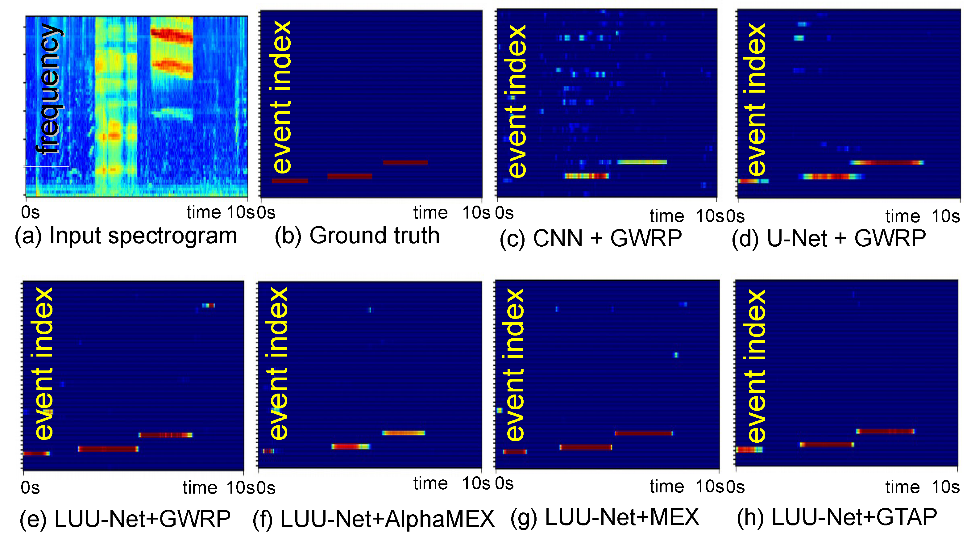
Figure 8 shows the sound event detection results with various models and various global pooling methods. The models in (c–e) were trained by the CNN, U-Net, and LUU-Net, respectively, and GWRP was adopted. In (c), event labels predicted by the CNN, the first event was almost missing, and many falsely detected units were seen and scattered in the upper part of the figure. In (d), U-Net prediction, the first event was detected, and much fewer false prediction units were observed. In (e), by the proposed LUU-Net, the event labels were more clearly detected, and a very small amount of false predictions were observed. To show the differences of the global pooling methods, event prediction examples are shown in (f–h), whose models were configured with AlphaMEX, MEX, and the proposed GTAP, respectively. There was no noticeable difference between (e) GWRP and (g) MEX, but the first event was almost missing in (f) AlphaMEX. This explains the low F1 score of AlphaMEX in Table 9 for the SED task. In (h), the proposed GTAP with , the detection results were much more distinctive than the others, and the false predictions almost disappeared.
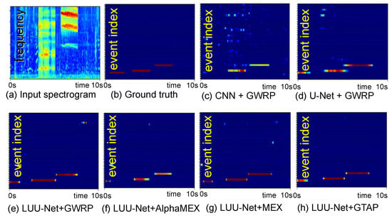
Figure 8.
Sound event detection examples with various models and global pooling methods. The vertical axis in (b–h) represents the class number. (a) Spectrogram of the input mixture sample generated by the original synthetic policy. The x-axis is the time in seconds (10 s long), and the y-axis is the frequency (only are shown). (b) Ground truth labels. There are 3 distinctive sound events, represented by bright red lines. For (b–h), the x-axis is the time in seconds aligned with the x-axis of the spectrogram in (a), and the y-axis represents the event labels. (c–h) display sound event labels predicted by (c) CNN with GWRP, (d) U-Net with GWRP, (e) LUU-Net with GWRP, (f) LUU-Net with AlphaMEX, (g) LUU-Net with MEX, and (h) LUU-Net with GTAP.
4.5. Longer Clipping Synthetic Policy
This section describes the experimental results on the dataset synthesized by the longer clipping policy given in Table 1. The mean and standard deviation of the event length included in this dataset were and s, respectively. The event length was limited to 5 s, so this dataset also included overlaps between events around 3 and s. The audio tagging (AT) and sound event detection (SED) results are shown in Table 10. Similar to the original synthetic policy, U-Net showed much higher tagging and detection performances ( and F1 scores), as well as reduced computational overhead. Comparing U-Net and LUU-Net, with the same GWRP, LUU-Net showed 0.7 higher tagging () and 0.6 lower detection () F1 scores. With longer event lengths, the proposed LUU-Net was less advantageous, except in the computational efficiency. This is because the model parameters of U-Net were better trained with longer event lengths, so more stable performance than that of the original synthetic policy was obtained. The tagging F1 scores of GWRP, AlphaMEX, and MEX with LUU-Net were all similar, but AlphaMEX showed lower detection performance than the other pooling methods.

For the CNN, U-Net, and LUU-Net, we applied the proposed GTAP with in terms of the mF1. There were huge performance degradations in the CNN with GTAP, similar to the original synthetic policy. Especially in SED, much higher precision was obtained, but recall dropped drastically. Because the proposed GTAP cuts off the output map, many activations were lost, and therefore, the recall metrics dropped greatly. With U-Net, little performance drops were observed with GTAP. With the proposed LUU-Net, GTAP improved both the AT and SED performances. The tagging F1 score with GWRP was and with GTAP with , , , and , respectively, so the best F1 score was obtained with , which is the same as the experimental results with the original synthetic policy. The detection F1 scores were , , and , respectively, and the best was also with . Interestingly, it was not as good as the other values in the original policy. However, was best in both the tagging and detection tasks. This implies that longer event lengths should provide more obvious unit labels and improve both tagging and detection performances.
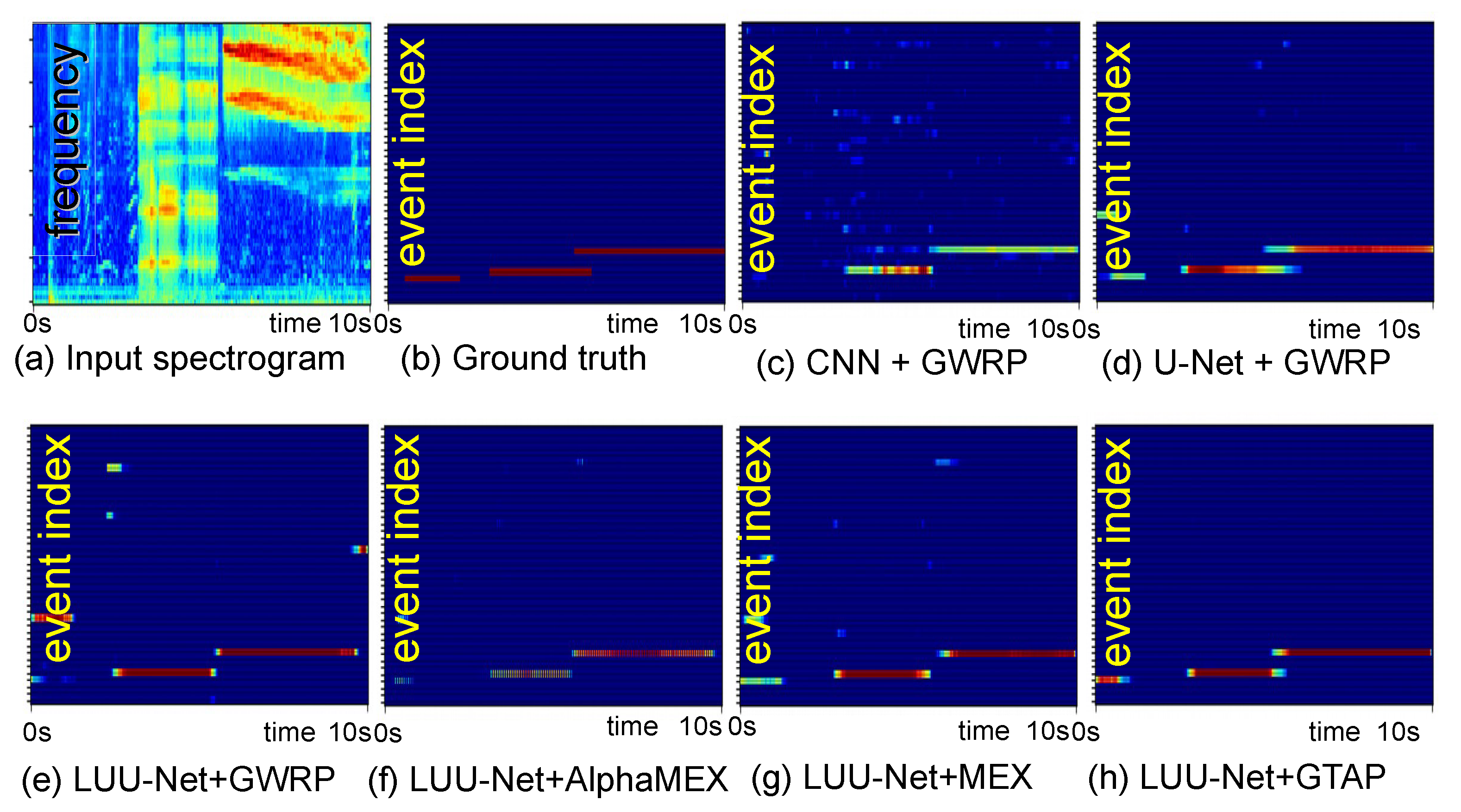
Figure 9 shows the sound event detection examples for the mixtures generated by the longer clipping policy. Various models and various global pooling methods were applied. The U-Net (d) and LUU-Net (e) results were better than those of CNN (c), but there were still prediction errors, as well as false detections. The proposed GTAP with (h) showed the best prediction performance. Almost no false predictions were observed, and the overlap between the second and the third events was also detected.
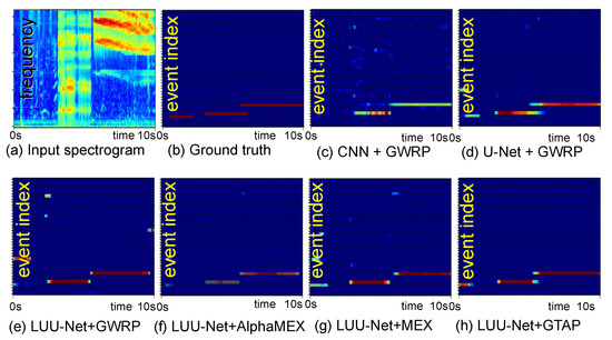
Figure 9.
Sound event detection examples with various models and global pooling methods. The vertical axis in (b–h) represents the class number. (a) Spectrogram of the input mixture sample generated by the longer clipping policy. (b) Ground truth labels. (c–h) display sound event labels predicted by (c) CNN with GWRP, (d) U-Net with GWRP, LUU-Net with (e) GWRP, (f) AlphaMEX, (g) MEX, and (h) GTAP. The x-axis is the time in seconds, and the y-axis represents the frequency (a) or event labels (b–h). Sound event detection examples with CNN, U-Net, and LUU-Net with GWRP.
4.6. Random Onset Synthetic Policy
Table 11 shows the audio tagging and sound event detection results of the dataset synthesized by the random onset policy in Table 1. The maximum event length was set to be 2.0 s, and the mean and standard deviation of the event length were 1.7 and 0.51 s, which were the same as the original synthetic policy. In the original policy, the event onset and offset times were configured so that there should not be any overlap. However, the random onset policy does not have such requirements, so there were significantly many overlaps among the events. In Table 11, U-Net with GWRP showed tagging and detection F1 scores, which were much lower than the and for the original policy. By using the proposed LUU-Net, the F1 scores were and , which were and higher than those of U-Net. U-Net showed good recall scores in both the tagging and detection tasks, but other measures were lower than LUU-Net. The number of steps increased from to , so LUU-Net was -times faster than U-Net. GWRP showed a good F1 score, which was similar to MEX, but the iteration speed was about 30% slower because of sorting.

The last 3 rows use the proposed GTAP with . The tagging F1 scores were , , and , respectively. The best and the second-best F1 scores were obtained with and , respectively, which were the same as the original policy. However, the F1 score difference was much less: original policy and random onset . The detection F1 scores were , , and , respectively. The sum of the F1 scores of the tagging and detection tasks was with and with . Therefore, the value that showed a higher sum of F1 scores and well-balanced performances in the tagging and detection tasks was .
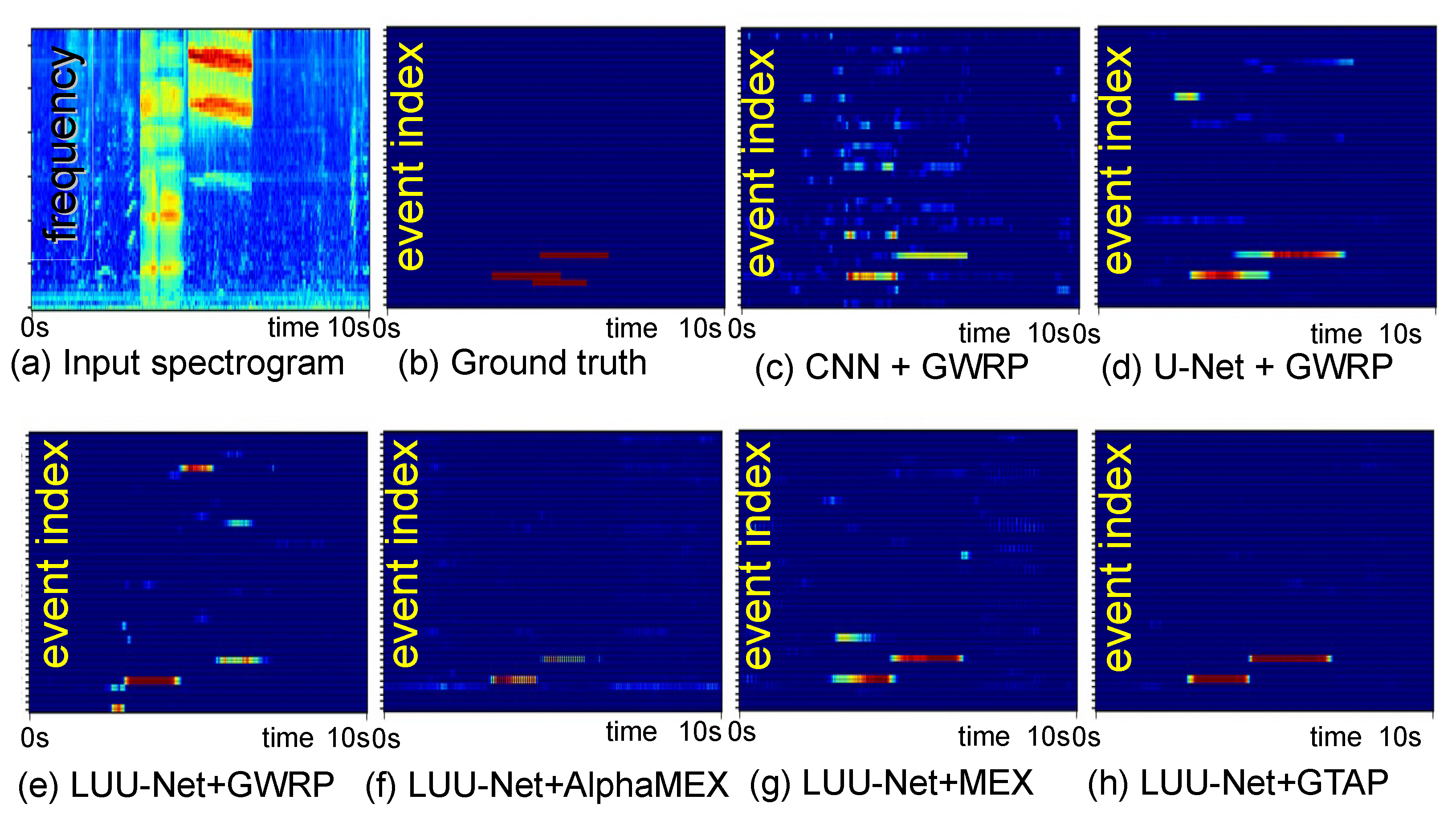
Figure 10 shows the sound event detection examples for the mixtures generated by the random onset synthetic policy. Various models and various global pooling methods were applied. In the CNN detection example in (c), there were many false detections scattered in the segmentation map. As shown in (d,e), U-Net and LUU-Net provided relatively clean detection results, but there were still many false detections. In (f,g), using AlphaMEX and MEX, it can be seen that the false detections mostly disappeared. In (h), using the proposed GTAP with , it provided very clean detection results.
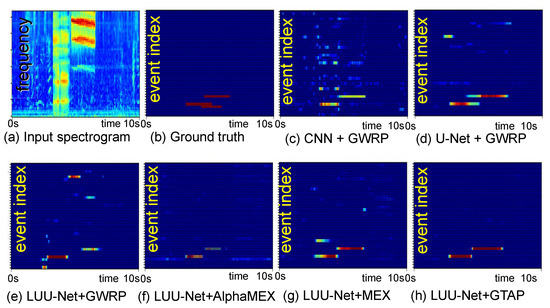
Figure 10.
Sound event detection examples with various models and global pooling methods. The vertical axis in (b–h) represents the class number. (a) Spectrogram of the input mixture sample generated by the random onset policy. (b) Ground truth labels. (c–h) display sound event labels predicted by (c) CNN with GWRP, (d) U-Net with GWRP, LUU-Net with (e) GWRP, (f) AlphaMEX, (g) MEX, and (h) GTAP. The x-axis is the time in seconds, and the y-axis represents the frequency (a) or event labels (b–h).
4.7. Mixed Synthetic Policy
Table 12 shows the audio tagging and sound event detection results of the dataset synthesized by the mixed policy in Table 1. The maximum event length was set to be s, and the mean and standard deviation of the event length were and s, respectively. The mean length was seconds shorter than the longer policy because there were more chances of sound events being cut off. This was the most-difficult dataset, so the F1 scores were overall much lower than the other synthetic policies. First, in the first 3 rows, we compare the CNN, U-Net, and the proposed LUU-Net with the GWRP method. Both U-Net and LUU-Net were much better than the CNN in both the tagging and detection F1 scores. LUU-Net was slightly better than U-Net, with a -times faster training speed. Comparing GWRP, AlphaMEX, and MEX, they showed similar performances in tagging, but AlphaMEX was the worst at detection. Lastly, we compared different values of the hyperparameter with the proposed GTAP method. In tagging, showed a higher F1 than , and showed a higher F1 than . The sum of F1 scores was with , so was the best value for the mixed synthetic policy. The number of steps increased from the of U-Net to the of LUU-Net with GTAP, so the proposed method was about 4-times faster.

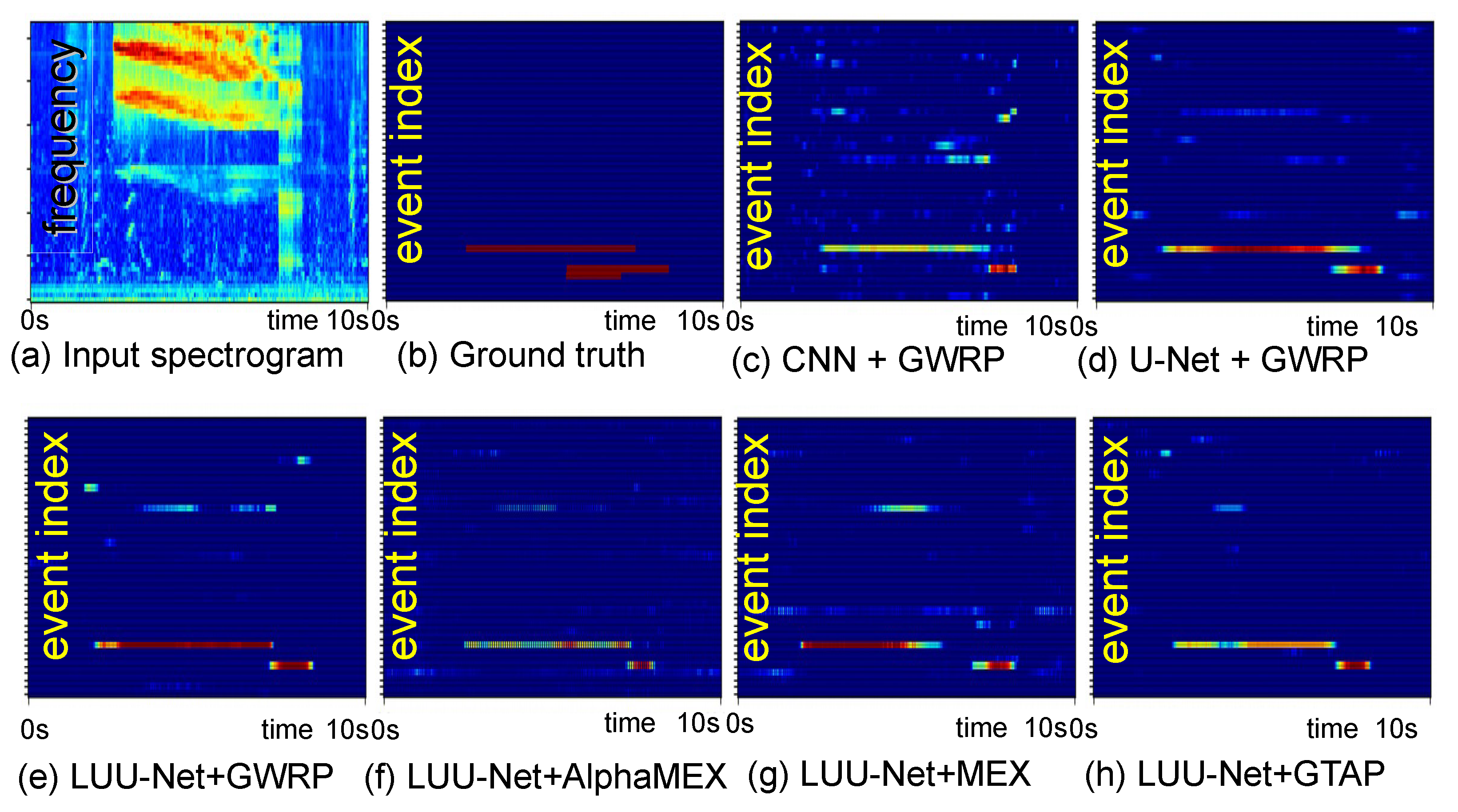
Figure 11 shows the sound event detection examples for the mixtures generated by the mixed synthetic policy. Various models and various global pooling methods were applied. In the CNN detection example in (c), there were many false detections scattered in the segmentation map. As shown in (d,e), U-Net and LUU-Net provided relatively clean detection results, but there were still many false detections. In (f,g), using AlphaMEX and MEX, it can be seen that the false detections mostly disappeared. In (h), using the proposed GTAP with , it provided very clean detection results.
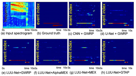
Figure 11.
Sound event detection examples with various models and global pooling methods. The vertical axis in (b–h) represents the class number. (a) Spectrogram of the input mixture sample generated by the mixed synthetic policy. (b) Ground truth labels. (c–h) display sound event labels predicted by (c) CNN with GWRP, (d) U-Net with GWRP, LUU-Net with (e) GWRP, (f) AlphaMEX, (g) MEX, and (h) GTAP. The x-axis is the time in seconds, and the y-axis represents the frequency (a) or event labels (b–h).
4.8. Summary of Experimental Results
As shown in Table 9, Table 10, Table 11 and Table 12, the proposed methods improved the audio tagging and sound event detection performances in most of the cases. Comparing U-Net and the proposed LUU-Net with the same GWRP, LUU-Net improved the tagging F1 score by up to 1.7% and the detection score by up to 1.5%. The training became more than three-times faster. In summary, the proposed LUU-Net slightly improved the tagging and detection performances with much faster model learning. Looking into the detailed precision and recall scores, an interesting property was observed. In all four synthetic cases (original, longer clipping, random onset, and mixed), U-Net with GWRP usually showed relatively low precision scores and high recall scores when compared to those of LUU-Net with the same global pooling. Because the sound event onset timings were the same for all the frequency units, the segmentation targets should be varied in time only. The limited upsampling in the LUU-Net decoder provided blocked averaging in the frequency axis, resulting in low frequency resolution. A lower resolution is less likely to be affected by outliers, and LUU-Net did not change the time resolution, so there was no difference in the detection targets. This explains the high precision scores of LUU-Net. On the contrary, lower resolution is less effective in the precise exclusion of false units, so the recall scores of LUU-Net were lower than U-Net. This property appeared in all of the global pooling methods with LUU-Net. If the given application requires higher precision than recall, i.e., higher true detection rate, LUU-Net is preferred.
The proposed GTAP also improved the tagging F1 score by up to 4.6 and the detection F1 score by up to 5.2 with appropriate selections of the hyperparameter . In audio tagging tasks where the outputs were directly used in computing the training loss, its value was more effective than the sound event detection tasks. Generally, with small values, for example if we compare the results of with those of in our experiments, relatively high precision and low recall scores of the audio tagging tasks were observed. According to Equation (7), the threshold becomes smaller as becomes smaller, more units are chosen to be averaged in Equation (5), and the average is used for computing the classification loss. Therefore, about 10% higher precision scores were obtained for all four synthetic datasets, as shown in Table 9, Table 10, Table 11 and Table 12. However, the recall scores were about 7–10% lower, resulting in 2.1–4.6% higher F1 scores because of the higher false positive rates. For , it also showed higher precision and lower recall scores than those of , but the differences were not large enough to make a general statement. In the sound event detection tasks, opposite results were observed. Comparing the results of with those of , relatively low precision and high recall scores were observed. Precisely speaking, when compared to , there were 10.4–23.9% lower precision and 5.9–8.6% higher recall scores, resulting in up to 6.0% lower F1 scores. When , there were 2.2–4.6% higher precision and 2.0–3.6% lower recall scores, and the F1 scores were up to 1.8% higher. This can be explained by the fact that the prediction of segmentation masks was not directly used for the computation of the target loss function. The learning process did not directly improve the prediction accuracy of the segmentation, which was not tightly related to the combination of the precision and recall scores, but the individual scores, so it can be biased to either the recall or prediction. The combined F1 scores were best with , except the random onset dataset, because it provided a well-balanced prediction of the segmentation masks in a weakly supervised manner.
5. Discussion
We analyzed the experimental results to show the detailed contributions of the proposed LUU-Net and GTAP. The experimental results in Table 9, Table 10, Table 11 and Table 12 are drawn as graphical charts for better visualization and analysis.
5.1. Execution Time Comparison
Figure 12 visualizes the differences of the number of steps per unit second. Comparing the CNN and LUU-Net, the training time of LUU-Net was about eight-times faster in most cases. Comparing U-Net and LUU-Net, it was about three-times faster. Because LUU-Net reduces the output map sizes by , , and in the decoder part, the computation time was reduced drastically. There were no notable differences among the synthetic policies. Comparing GWRP and GTAP, GTAP was about 1.2-times faster with the CNN and LUU-Net and 1.4-times faster with U-Net. Because about half of the output map components were discarded at the final output layer with GTAP, this improvement in time with GTAP is reasonable. Combining GTAP with LUU-Net, a 4-times improvement in the execution time over GWRP with U-Net and up to 10-times over GWRP with the CNN were expected.

Figure 12.
Comparison of the number of steps per unit second. The first two sets of bars represent the CNN with GWRP and GTAP, with 4 bars measured from the original, longer clips, random onsets, and mixed synthetic policies. The second two sets of bars represent U-Net, and the third two sets of bars are for LUU-Net.
5.2. Audio Tagging Performance Comparison
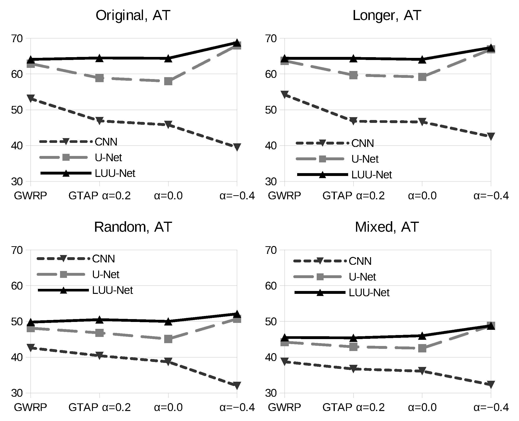
To show the performance variations with the change of the models and pooling methods under different conditions, the mean F1 scores from Table 9, Table 10, Table 11 and Table 12 are drawn as two-dimensional charts. Figure 13 shows the average F1 scores for audio tagging tasks with the original, longer clipping, random onsets, and mixed synthetic policies. In all of the policies, the performances of GWRP and GTAP on the U-Net and LUU-Net were almost the same, but there was a 3–5% drop with GTAP and GTAP on U-Net. Those performance drops were not observed for LUU-Net, so relative improvements were obtained with GTAP and GTAP. For the CNN, there was too much degradation with GTAP compared to GWRP. The baseline CNN design in Table 4 does not have any bottleneck layer, which compresses the information from the input, so the output map pruning in GTAP resulted in information loss. Among the GTAP methods, was the best with both U-Net and LUU-Net. In most of the cases, the proposed LUU-Net was superior to the conventional U-Net, and the proposed GTAP was slightly better than the conventional GWRP.
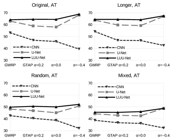
Figure 13.
Audio tagging (AT) performance comparison with various deep learning models, pooling methods, and training data generation policies. Average F1 scores drawn; the x-axis is pooling methods; lines are CNN, U-Net, and LUU-Net. The individual charts are the results with the original, longer clipping, random onsets, and mixed synthetic policies.
5.3. Sound Event Detection Performance Comparison
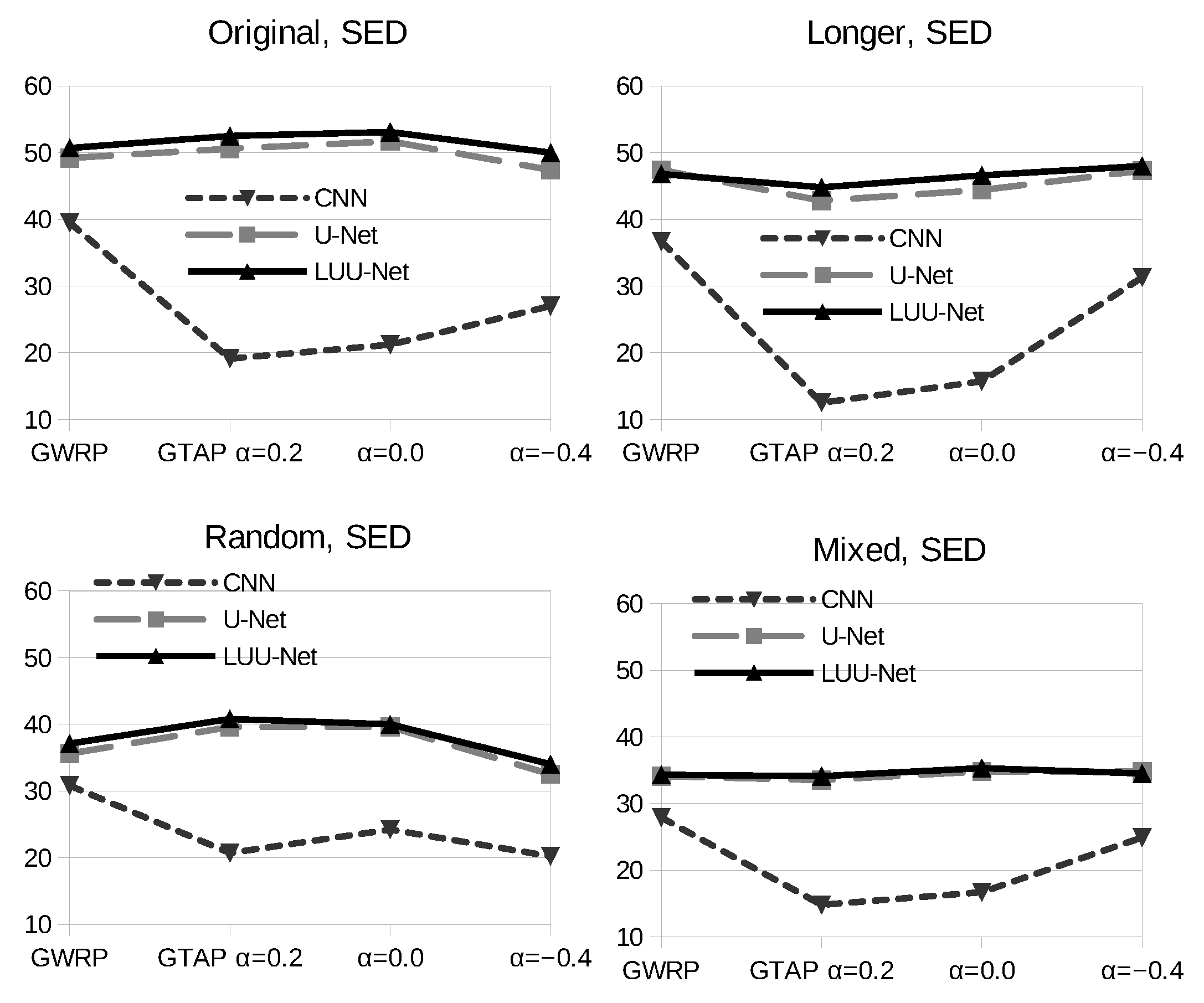
A similar chart is drawn with the SED tasks in Figure 14. In all cases, except GWRP and the longer clipping policy, LUU-Net outperformed U-Net and the CNN. For the original and random policies, where the audio clip lengths were less than 2 s, GTAP with was better than and GWRP. For the longer and mixed policies with longer audio clips lengths, less than 5 s, GTAP with was not as good as GWRP and GTAP with . Longer clip lengths require larger amounts of activation, so a smaller value of is more suited to the longer and mixed policies.
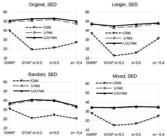
Figure 14.
Sound event detection (SED) performance comparison with various deep learning models, pooling methods, and training data generation policies by average F1 scores.
5.4. Further Analysis of LUU-Net Results
Figure 13 and Figure 14 show that the proposed LUU-Net and GTAP improved both the audio tagging and sound event detection performances over the conventional U-Net and GWRP. However, it is difficult to choose an optimal value for the hyperparameter , so that it works best with all the experimental conditions. Therefore, we made a detailed analysis of the experimental results of LUU-Net with GTAP to find a relationship of the hyperparameter and audio mixing conditions.
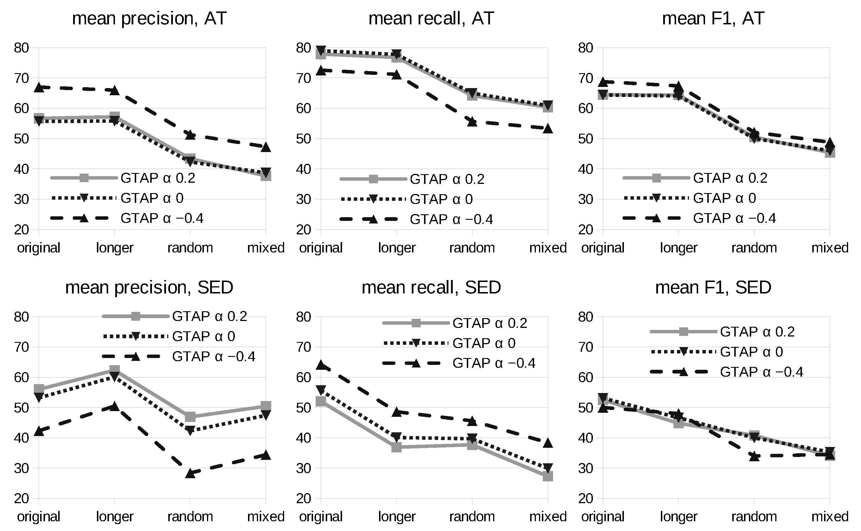
Figure 15 shows the AT and SED results of LUU-Net only. All the performance metrics, precision, recall, and F1 scores are drawn. For the mean precision, AT, was the best among the three values for all mixing conditions. For the mean recall, AT, was the best and the worst. Combining the precision and recall, the F1 scores of were overall the best. In the SED tasks, the opposite observation was made. is the worst in the precision scores and was the best in recall scores. The combined F1 scores were almost the same for all three values. If in Equation (7), more output map values were chosen to compute the class label predictions for the whole clip in the AT tasks. Having more output map components, the class activation information was kept more in the pooling, so higher precision was obtained. For the SED tasks, the performance metrics were computed as segment-based, so more output map components would lead to higher false positive rates. Therefore, lower precision is obtained by Equation (8). The opposite explanation can be applied to the lower recall scores on the AT tasks with and the higher recall scores on the SED tasks. In Equation (), reducing false negatives is directly related to higher recall scores. A larger amount of output maps in GTAP with would lead to less inclusion of inactive outputs, so higher recall scores were observed in the SED tasks computed in a segment-based manner.
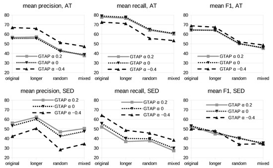
Figure 15.
Illustrations of audio tagging and sound event detection performances by varying audio mixing conditions. The subfigures on the left are graphical charts of average precision scores of GTAP with . The x-axis is the audio synthetic policies. The upper chart is audio tagging performances, and the lower one is sound event detection performances. The subfigures at the center are graphical charts of the average recall scores, and those on the right are the average F1 scores.
In summary, the proposed LUU-Net with GTAP was better than the conventional U-Net with GWRP in most cases. The proposed GTAP can be configured to provide versatile choices of target applications by varying a single hyperparameter . A smaller threshold by a negative value is suggested when higher audio tagging performance is required, i.e., the identities of the audio sources are more important. When a higher recall rate in tagging or better sound event detection performance is required, choosing is suggested.
5.5. Code Availability
All the source codes for training the models and performing the experiments are publicly available at https://github.com/lsw0767/SED (accessed on 29 May 2023). The source dataset was taken from the DCASE 2018 Challenge, which is accessible at https://dcase.community/challenge2018 (accessed on 18 February 2023).
6. Conclusions
In this paper, we proposed two methods to improve the performance of weakly supervised sound event detection. The first method was a modification of the conventional U-Net to perform limited upscaling (LUU-Net). Assuming that the upscaling function along the frequency axis of the U-Net is not necessary in sound event detection, upsampling gradually to the original size was applied to the time domain only. The second method was global threshold average pooling (GTAP), which replaced the conventional global weighted rank pooling (GWRP). GWRP showed higher detection performance compared to global average pooling (GAP) and global max pooling (GMP) [16]. However, GWRP requires output map sorting in every pooling step. The proposed GTAP eliminates the sorting operation and replaces it with simple thresholding. To find the threshold, the mean and the standard deviation of the output feature map are necessary, which are much more computationally efficient than sorting. GTAP performs the global pooling by calculating the average of only the value above a certain threshold by using the characteristic that the rank-based weight of GWRP almost ignores smaller values. There was a significant improvement in training speed, with small or huge performance improvements depending on the mixing conditions. According to the experimental results, the proposed LUU-Net with GTAP greatly outperformed the CNN and U-Net in various mixing datasets. The advantage of applying the proposed LUU-Net is the improved computation time. The amount of model parameters was about 40% of the conventional U-Net, and the measured training time was 3-times faster than U-Net and 8-times faster than the baseline CNN. With the proposed GTAP, an additional 1.2-times faster speed was obtained. In terms of audio tagging and sound event detection performance, the proposed LUU-Net outperformed the U-Net and the CNN in almost all cases. Another advantage of the proposed GTAP is that, by varying a single hyperparameter, it can be adapted to various target applications with different requirements. As a conclusion, the major contribution of the proposed LUU-Net and GTAP is the reduction of the computation time without any performance loss. Future work includes the automatic adaptation of the hyperparameter for real applications.
Author Contributions
Conceptualization, S.L., H.K., and G.-J.J.; methodology, S.L.; software, S.L.; validation, S.L. and G.-J.J.; formal analysis, S.L. and H.K.; investigation, H.K.; resources, G.-J.J.; data curation, S.L.; writing–original draft preparation, S.L.; writing–review and editing, H.K. and G.-J.J.; visualization, S.L.; supervision, G.-J.J.; project administration, G.-J.J.; funding acquisition, G.-J.J. All authors have read and agreed to the published version of the manuscript.
Funding
This research was supported by the Culture, Sports and Tourism R&D Program through the Korea Creative Content Agency grant funded by the Ministry of Culture, Sports and Tourism in 2022 (project name: Development of high-speed music search technology using deep learning; project number: CR202104004).
Institutional Review Board Statement
Not applicable.
Informed Consent Statement
Not applicable.
Data Availability Statement
The original audio data are available at https://dcase.community/challenge2018 (accessed on 18 February 2023). Newly created data such as audio labels and Source codes are available at https://github.com/lsw0767/SED (accessed on 29 May 2023).
Conflicts of Interest
The authors declare no conflict of interest.
Abbreviations
The following abbreviations are used in this manuscript:
| SED | Sound event detection |
| CNN | Convolutional neural network |
| RNN | Recurrent neural network |
| VGG | Visual geometry group |
| GAP | Global average pooling |
| GMP | Global max pooling |
| GWRP | Global weighted rank pooling |
| GTAP | Global threshold average pooling |
References
- Mesaros, A.; Heittola, T.; Virtanen, T.; Plumbley, M.D. Sound event detection: A tutorial. IEEE Signal Process. Mag. 2021, 38, 67–83. [Google Scholar] [CrossRef]
- Parascandolo, G.; Huttunen, H.; Virtanen, T. Recurrent neural networks for polyphonic sound event detection in real life recordings. In Proceedings of the IEEE International Conference on Acoustics, Speech and Signal Processing (ICASSP), Shanghai, China, 20–25 March 2016; pp. 6440–6444. [Google Scholar]
- Sehgal, A.; Kehtarnavaz, N. A convolutional neural network smartphone app for real-time voice activity detection. IEEE Access 2018, 6, 9017–9026. [Google Scholar] [CrossRef] [PubMed]
- Sainath, T.; Parada, C. Convolutional Neural Networks for Small-Footprint Keyword Spotting; Google, Inc.: New York, NY, USA, 2015; pp. 1478–1482. [Google Scholar]
- Takahashi, N.; Gygli, M.; Pfister, B.; Van Gool, L. Deep convolutional neural networks and data augmentation for acoustic event detection. arXiv 2016, arXiv:1604.07160. [Google Scholar]
- Zhang, B.; Zhao, Q.; Feng, W.; Lyu, S. AlphaMEX: A smarter global pooling method for convolutional neural networks. Neurocomputing 2018, 321, 36–48. [Google Scholar] [CrossRef]
- Tarvainen, A.; Valpola, H. Mean teachers are better role models: Weight-averaged consistency targets improve semi-supervised deep learning results. Proc. Adv. Neural Inf. Process. Syst. 2017, 30, 1195–1204. [Google Scholar]
- Lu, R.; Duan, Z. Bidirectional GRU for sound event detection. In Proceedings of the Detection and Classification of Acoustic Scenes and Events 2018 Workshop (DCASE2017), Munich, Germany, 16 November 2017. [Google Scholar]
- JiaKai, L. Mean Teacher Convolution System for DCASE 2018 Task 4. In Proceedings of the Detection and Classification of Acoustic Scenes and Events 2018 Workshop (DCASE2018), Surrey, UK, 19–20 November 2018. [Google Scholar]
- Mesaros, A.; Heittola, T.; Virtanen, T. TUT database for acoustic scene classification and sound event detection. In Proceedings of the European Signal Processing Conference (EUSIPCO), Budapest, Hungary, 29 August–2 September 2016; pp. 1128–1132. [Google Scholar]
- Kumar, A.; Raj, B. Audio Event Detection using Weakly Labeled Data. arXiv 2016, arXiv:1605.02401. [Google Scholar]
- Turpault, N.; Serizel, R.; Parag Shah, A.; Salamon, J. Sound event detection in domestic environments with weakly labeled data and soundscape synthesis. In Workshop on Detection and Classification of Acoustic Scenes and Events; HAL: Bengaluru, India, 2019. [Google Scholar]
- Salamon, J.; MacConnell, D.; Cartwright, M.; Li, P.; Bello, J.P. Scaper: A Library for Soundscape Synthesis and Augmentation. In Proceedings of the IEEE Workshop on Applications of Signal Processing to Audio and Acoustics (WASPAA), New Paltz, NY, USA, 15–18 October 2017. [Google Scholar]
- McFee, B.; Salamon, J.; Bello, J.P. Adaptive pooling operators for weakly labeled sound event detection. IEEE/ACM Trans. Audio Speech Lang. Process. 2018, 26, 2180–2193. [Google Scholar] [CrossRef]
- Pankajakshan, A.; Bear, H.L.; Benetos, E. Polyphonic Sound Event and Sound Activity Detection: A Multi-task approach. In Proceedings of the IEEE Workshop on Applications of Signal Processing to Audio and Acoustics (WASPAA), New Paltz, NY, USA, 20–23 October 2019. [Google Scholar]
- Kong, Q.; Xu, Y.; Sobieraj, I.; Wang, W.; Plumbley, M.D. Sound Event Detection and Time–Frequency Segmentation from Weakly Labelled Data. IEEE/ACM Trans. Audio Speech Lang. Process. 2019, 27, 777–787. [Google Scholar] [CrossRef]
- Pandeya, Y.R.; Bhattarai, B.; Lee, J. Visual Object Detector for Cow Sound Event Detection. IEEE Access 2020, 8, 162625–162633. [Google Scholar] [CrossRef]
- Kolesnikov, A.; Lampert, C.H. Seed, expand and constrain: Three principles for weakly-supervised image segmentation. In Proceedings of the European Conference on Computer Vision, Amsterdam, The Netherlands, 11–14 October 2016; Springer: Berlin/Heidelberg, Germany, 2016; pp. 695–711. [Google Scholar]
- Cai, Z.; Vasconcelos, N. Cascade R-CNN: Delving into high quality object detection. In Proceedings of the IEEE/CVF Conference on Computer Vision and Pattern Recognition (CVPR), Salt Lake City, UT, USA, 18–23 June 2018; pp. 6154–6162. [Google Scholar]
- Ren, S.; He, K.; Girshick, R.; Sun, J. Faster R-CNN: Towards real-time object detection with region proposal networks. IEEE Trans. Pattern Anal. Mach. Intell. 2017, 39, 1137–1149. [Google Scholar] [CrossRef] [PubMed]
- Zhou, B.; Khosla, A.; Lapedriza, A.; Oliva, A.; Torralba, A. Learning deep features for discriminative localization. arXiv 2016, arXiv:1512.04150. [Google Scholar]
- Dinkel, H.; Wu, M.; Yu, K. Towards duration robust weakly supervised sound event detection. IEEE/ACM Trans. Audio Speech Lang. Process. 2021, 29, 887–900. [Google Scholar] [CrossRef]
- Miyazaki, K.; Komatsu, T.; Hayashi, T.; Watanabe, S.; Toda, T.; Takeda, K. Weakly-supervised sound event detection with self-attention. In Proceedings of the IEEE International Conference on Acoustics, Speech and Signal Processing (ICASSP), Barcelona, Spain, 4–8 May 2020; pp. 66–70. [Google Scholar]
- Deshmukh, S.; Raj, B.; Singh, R. Improving Weakly Supervised Sound Event Detection with Self-Supervised Auxiliary Tasks; Google, Inc.: New York, NY, USA, 2021; pp. 596–600. [Google Scholar]
- Park, C.; Kim, D.; Ko, H. Sound Event Detection by Pseudo-Labeling in Weakly Labeled Dataset. Sensors 2021, 21, 8375. [Google Scholar] [CrossRef] [PubMed]
- Ronneberger, O.; Fischer, P.; Brox, T. U-net: Convolutional networks for biomedical image segmentation. In Proceedings of the International Conference on Medical Image Computing and Computer-Assisted Intervention, Munich, Germany, 5–9 October 2015; Springer: Berlin/Heidelberg, Germany, 2015; pp. 234–241. [Google Scholar]
- Chen, L.C.; Papandreou, G.; Kokkinos, I.; Murphy, K.; Yuille, A.L. DeepLab: Semantic Image Segmentation with Deep Convolutional Nets, Atrous Convolution, and Fully Connected CRFs. IEEE Trans. Pattern Anal. Mach. Intell. 2018, 40, 834–848. [Google Scholar] [CrossRef] [PubMed]
- Lin, M.; Chen, Q.; Yan, S. Network In Network. arXiv 2013, arXiv:1312.4400. [Google Scholar]
- Krizhevsky, A.; Sutskever, I.; Hinton, G.E. Imagenet classification with deep convolutional neural networks. Commun. ACM 2017, 60, 84–90. [Google Scholar] [CrossRef]
- Goodfellow, I.; Bengio, Y.; Courville, A. Deep Learning; MIT Press: Cambridge, MA, USA, 2016; Available online: http://www.deeplearningbook.org (accessed on 16 February 2023).
- Harris, S.L.; Harris, D.M. Digital Design and Computer Architecture; Elsevier: Amsterdam, The Netherlands, 2016. [Google Scholar] [CrossRef]
- Mesaros, A.; Heittola, T.; Virtanen, T. A multi-device dataset for urban acoustic scene classification. In Proceedings of the Detection and Classification of Acoustic Scenes and Events 2018 Workshop (DCASE2018), Surrey, UK, 19–20 November 2018; pp. 9–13. [Google Scholar]
- Fonseca, E.; Plakal, M.; Font, F.; Ellis, D.P.W.; Favory, X.; Pons, J.; Serra, X. General-purpose Tagging of Freesound Audio with AudioSet Labels: Task Description, Dataset, and Baseline. In Proceedings of the Detection and Classification of Acoustic Scenes and Events 2018 Workshop (DCASE2018), Surrey, UK, 19–20 November 2018; pp. 69–73. [Google Scholar]
- Ioffe, S.; Szegedy, C. Batch normalization: Accelerating deep network training by reducing internal covariate shift. arXiv 2015, arXiv:1502.03167. [Google Scholar]
- Nair, V.; Hinton, G.E. Rectified linear units improve restricted boltzmann machines. In Proceedings of the International Conference on Machine Learning (ICML-10), Madison, WI, USA, 21–24 June 2010; pp. 807–814. [Google Scholar]
- He, K.; Zhang, X.; Ren, S.; Sun, J. Deep residual learning for image recognition. arXiv 2015, arXiv:1512.03385. [Google Scholar]
- Cohen, N.; Sharir, O.; Shashua, A. Deep SimNets. arXiv 2015, arXiv:1506.03059. [Google Scholar]
- Powers, D.M.W. Evaluation: From Precision, Recall and F-Factor to ROC, Informedness, Markedness & Correlation. J. Mach. Learn. Technol. 2011, 2, 37–63. [Google Scholar]
Disclaimer/Publisher’s Note: The statements, opinions and data contained in all publications are solely those of the individual author(s) and contributor(s) and not of MDPI and/or the editor(s). MDPI and/or the editor(s) disclaim responsibility for any injury to people or property resulting from any ideas, methods, instructions or products referred to in the content. |
© 2023 by the authors. Licensee MDPI, Basel, Switzerland. This article is an open access article distributed under the terms and conditions of the Creative Commons Attribution (CC BY) license (https://creativecommons.org/licenses/by/4.0/).


