Building Ensemble of Resnet for Dolphin Whistle Detection

Abstract

Ecoacoustics is arguably the best method for monitoring marine environments, but analyzing and interpreting acoustic data has traditionally demanded substantial human supervision and resources. These bottlenecks can be addressed by harnessing contemporary methods for automated audio signal analysis. This paper focuses on the problem of assessing dolphin whistles using state-of-the-art deep learning methods. Our system utilizes a fusion of various resnet50 networks integrated with data augmentation (DA) techniques applied not to the training data but to the test set. We also present training speeds and classification results using DA to the training set. Through extensive experiments conducted on a publicly available benchmark, our findings demonstrate that our ensemble yields significant performance enhancements across several commonly used metrics. For example, our approach obtained an accuracy of 0.949 compared to 0.923, the best reported in the literature. We also provide training and testing sets that other researchers can use for comparison purposes, as well as all the MATLAB/PyTorch source code used in this study.

1. Introduction

Marine ecosystems play a critical role in maintaining the balance of our planet’s ecosystem by supporting food security and contributing to climate regulation [1], making their preservation essential for the long-term sustainability of the earth’s environment. Thus, there is a growing need to develop and test innovative monitoring systems to ensure the natural preservation of marine habitats. Modern technologies have already shown great potential in monitoring habitats and advancing our understanding of marine communities [2]. Acoustic methods are commonly used for underwater investigations because they can detect and classify sensitive targets, even in low visibility conditions. Passive acoustic technologies (PAM), such as underwater microphones, or hydrophones, are particularly attractive, as they allow for non-invasive continuous monitoring of marine ecosystems without interfering with biological processes [3]. PAM has been shown to achieve various research and management goals by effectively detecting animal calls [4]. These objectives may include tracking and localizing animals [5,6], species identification, identifying individuals [3,7], analyzing distributions and behavior [8], and estimating animal density [9].

The bottlenose dolphin (Tursiops truncatus) is a highly intelligent marine mammal and a critical species for researchers studying marine ecosystems [10]. Like many other marine mammals, dolphins are acoustic specialists that rely on sounds for communication, reproduction, foraging, and navigational purposes. The acoustic communication of dolphins employs a wide range of vocalizations, including clicks, burst-pulses, buzzes, and whistles [11]. Whistles, in particular, serve various social functions such as individual identification, group cohesion, and coordination of activities, such as feeding, resting, socializing, and navigation [12]. Understanding and accurately detecting dolphin vocalizations is essential for monitoring their populations and assessing their role within marine ecosystems.

Traditional bioacoustics tools and algorithms for detecting dolphins have relied on spectrogram analysis, manual signal processing, and statistical methods [13]. For example, the reference approach pursued in [14] applies three noise removal algorithms to the spectrogram of a sound sample. Then, a connected region search is conducted to link together sections of the spectrogram that are above a predetermined threshold and close in time and frequency. A similar technique exploits a probabilistic Hough transform algorithm to detect ridges similar to thick line segments, which are then adjusted to the geometry of the potential whistles in the image via an active contour algorithm [15]. Other algorithmic methods aim to quantify the variation in complexity (randomness) occurring in the acoustic time series containing the vocalization; for example, by measuring signal entropy [16]. While these techniques have helped the study of dolphin vocalizations, they can be time-consuming and may not always provide accurate results due to the complexity and variability of the signals. Researchers have thus turned to machine learning methods to improve detection accuracy and efficiency.

Early machine learning studies in the field of dolphin detection applied traditional classifiers, such as Hidden Markov Models (HMM) [17] and Support Vector Machines (SVMs) [18]. For instance, in [19], a hidden Markov model was utilized for whistle classification, and in [20], classification and regression tree analysis was employed along with discriminant function analysis for categorizing parameters extracted from whistles. In [21], a multilayer perceptron classifier was implemented for classifying short-time Fourier transforms (STFTs) and wavelet transform coefficient energies of whistles. Lastly, in [15] a random forest algorithm and a support vector machine were combined to classify features derived from the duration, frequency, and cepstrum domain of whistles (see [22] for a review of the early literature).

More recently, researchers have employed deep learning methods to detect whistle vocalizations. Deep neural networks have demonstrated great potential in general sound detection [23] and specific underwater acoustic monitoring [24]. The Convolutional Neural Network (CNN) is one of the best-known deep learners. Though commonly considered an image classifier, CNNs have been applied to whale vocalizations, significantly reducing the false-positive rates compared to traditional algorithms, while at the same time enhancing call detection [25,26]. In [27], the authors compared four traditional methods for detecting dolphin echolocation clicks with six CNN architectures, demonstrating the superiority of the CNNs. In [28], CNNs were shown to outperform human experts in dolphin call detection accuracy. CNNs have also been applied to automatically categorize dolphin whistles into distinct groups, as in [29], and to extract whistle contours either by leveraging peak tracking algorithms [30] or by training CNN-based models for semantic segmentation [31].

Several studies of dolphin whistle classification have used data augmentation on the training set to enhance the performance of CNNs by reducing overfitting and increasing the size and variability of the available datasets [29,30,32]. Dolphin vocalizations are complex and highly variable, as analyzed in [33]. Unsurprisingly, some traditional music data augmentation methods, such as pitch shifting, time stretching, and adding background noise, have proven effective at this classification task. When synthesizing dolphin calls, care should be taken to apply augmentations to the audio signal rather than to the spectrograms, since altering the spectrogram could distort the time–frequency patterns of dolphin whistles, which would result in the semantic integrity of the labels being compromised [29,34]. In [29], primitive shapes were interjected into the audio signal to generate realistic ambient sounds in negative samples, and classical computer vision methods were used to create synthetic time–frequency whistles, which replaced the training data. Generative Adversarial Networks (GANs) have also been employed to generate synthetic dolphin vocalizations [32]. This research underscores the efficacy of data augmentation and synthesis methods in enhancing both the precision and stability of dolphin whistle categorization models, especially in situations where the datasets are restricted or imbalanced.

The goal of this work is to continue exploring data augmentation techniques for the task of dolphin vocalization detection. To this end, we use the benchmark dolphin whistles dataset developed by Korkmaz et al. [28], but apply data augmentation to the original test set of spectrograms to enlarge it rather than the training set. The training set contains all the spectrograms obtained from audio files recorded between 24 June and 30 June, while the test set is composed of the spectrograms of audio files recorded between 13 July and 15 July, a three-day window. Aside from augmenting the test set, we extract a three-day window (24–26 June) from the training set as the validation set.

The proposed system outperforms previous state-of-the-art methods on the same dataset using the same testing protocol. We find our results interesting, especially since many misclassified audio samples are unclassifiable, even by humans. Therefore, the classification result of our method is likely very close to maximum performance (AUC = 1 is not obtainable).

The main contributions of this study are the following:

• The creation of a new baseline on this benchmark (note: using data augmentation on the testing set increased performance);
• Clear and repeatable criteria for testing various new developments in machine learning on this dataset by providing fixed training and test sets (both augmented and not augmented) rather than a protocol involving randomization;
• Access to all the MATLAB/PyTorch source code used in this study https://github.com/LorisNanni/ (accessed on 7 July 2023).

The remainder of this paper is organized into three sections. In Section 2, we present the material and methods, and Section 2.1 and Section 2.2 provide a complete description of the dataset and baseline method presented in [28]. In Section 2.3, we offer a detailed account of our proposed approach. In Section 3, we present the results of tests comparing a standard ResNet with a set of ensembles, a comparison of our best ensemble with the state-of-the-art, and the results of using data augmentation on both the training and the test set. The conclusion in Section 4 discusses the shortcomings with the benchmark dataset and suggestions for further research.

2. Materials and Methods

2.1. Dataset

In this section, we describe the dataset developed by Korkmaz et al. [28] and detailed in that paper. The dataset contains 108,317 spectrograms, of which 49,807 are tagged as noise and 58,510 as dolphin whistles. The test set contains 6869 spectrograms. The data were collected with hydrophones during the summer of 2021 for 27 days from the dolphin’s reef in Eilat, Israel. Following retrieval, a quality assurance (QA) process was conducted on the data to eliminate occasional disruptions and prolonged periods of noise. This QA procedure included the elimination of noise transients through wavelet denoising and the identification and removal of cut-off events via thresholding and bias reduction.

2.1.1. Data Preprocessing and Tagging

As described in [28], the collected data were subjected to a bandpass filter in the range of 5–20 kHz to align with the majority of dolphins’ whistle vocalizations. The data were then passed through a whitening filter designed to rectify the hydrophone’s open circuit voltage response ripples and the sensitivity of the sound card. The recorded audio files, which consisted of two channels, were averaged before the creation of spectrograms to decrease noise. In addition, the preprocessing pipeline eliminated signal outliers based on their length using the quartiles-based Tukey method [35], which led to the exclusion of signals that were longer than 0.78 s and shorter than 0.14 s.

The short-time fast Fourier transform of the signal was computed using MATLAB’s spectrogram function from the digital signal processing toolbox to create the dolphin whistle spectrograms. SFFT was performed with a Blackman function window with 2048 points, periodic sampling, and a hop size achieved by multiplying the window length by 0.8. The subsequent spectrograms were computed by shifting the signal window by 0.4 s. These spectrogram images were finalized by applying a gray-scale colormap, converting the frequency to kHz and the power spectrum density to dB, and restricting the y-axis between 3 and 20 kHz to emphasize the most significant (dominant) frequency range [36].

The spectrograms were then manually labeled by a human expert in two steps: initial tagging and validation tagging. The first step involved precise annotation of 5 s spectrograms over ten days of data collection, which were used to train an initial version of a deep learning classifier. This classifier was then used to select new portions of recordings containing potential dolphin sounds, which made tagging the remaining data in the validation phase more efficient. The validation phase only required the verification of positive samples detected by the preliminary deep learning classifier.

A human expert was tasked with identifying dolphin whistles as curving lines in the time–frequency domain and disregarding the contour lines generated by shipping radiated noise. When the discrimination process was complex, the expert directly listened to the recorded audio track to identify whistle-like sounds. The tagging resulted in a binary classification (whistle vs. noise) and a contour line marking the time–frequency characteristic of the identified whistle. This contour was used to assess the quality of the manual tagging by ensuring that the bandwidth of the identified whistle fell within the expected thresholds for a dolphin’s whistle, specifically between 3 and 20 kHz. A second quality assessment was conducted by measuring the variance of the acoustic intensity of the identified whistle along the time–frequency contour, where the acoustic intensity of a valid whistle was expected to be stable.

2.1.2. Original Training and Test Sets

As mentioned in the introduction, the training set [28] contained all the spectrograms obtained from audio files recorded between 24 June and 30 June, while the test set was composed of the spectrograms of audio files recorded between 13 July and 15 July, a three-day window. The rationale given by the authors for dividing the training and test sets in this manner was primarily to test the generalizability of models using completely disparate sets of recordings, as this would better assess the detection accuracy amidst varying sea conditions.

As detailed in Section 2.3, we extracted a validation set from the training set obtained from audio files recorded between 24 June and 26 June. We used the validation set for learning the weights of the weighted sum rule, and then the whole training set was fed into the networks for classifying the test set.

2.2. Baseline Detection

PamGuard [14] is a widely used software designed to automatically recognize marine mammal vocalizations. It provides an interesting baseline method since it is widely used. The operational parameters of PamGuard were used as follows:

• The “Sound Acquisition” module from the “Sound Processing” section was included to manage the data acquisition device and convey its data to other modules;
• The “FFT (spectrogram) Engine” module from the “Sound Processing” section was incorporated to calculate spectrograms;
• The “Whistle and Moan Detector” module from the “Detectors” section was added for detecting dolphin whistles;
• The “Binary Storage” module from the “Utilities” section was incorporated to preserve information from various modules;
• A new spectrogram display was created by adding the “User Display” module from the “Displays” section.

Input spectrograms were devised utilizing the FFT analysis mentioned above with identical parameters: FFT window length was assigned 2048 points, and the hop size was set to the length multiplied by 0.8 using the Blackman window in the “FFT (spectrogram) Engine” module under the software settings. The frequency range was determined between 3 and 20 kHz, and the “FFT (spectrogram) Engine Noise free FFT data” was chosen as the source of FFT data in the “Whistle and Moan Detector” module settings. During the creation of a new spectrogram display, the number of panels was assigned as 2 to visualize both channels. A detection by PamGuard was classified as a true positive if the signal window identified by the software overlapped with at least 5% of the ground truth signal interval. While this criterion may appear lenient, it allowed for the inclusion of many PamGuard detections that might have otherwise been disregarded.

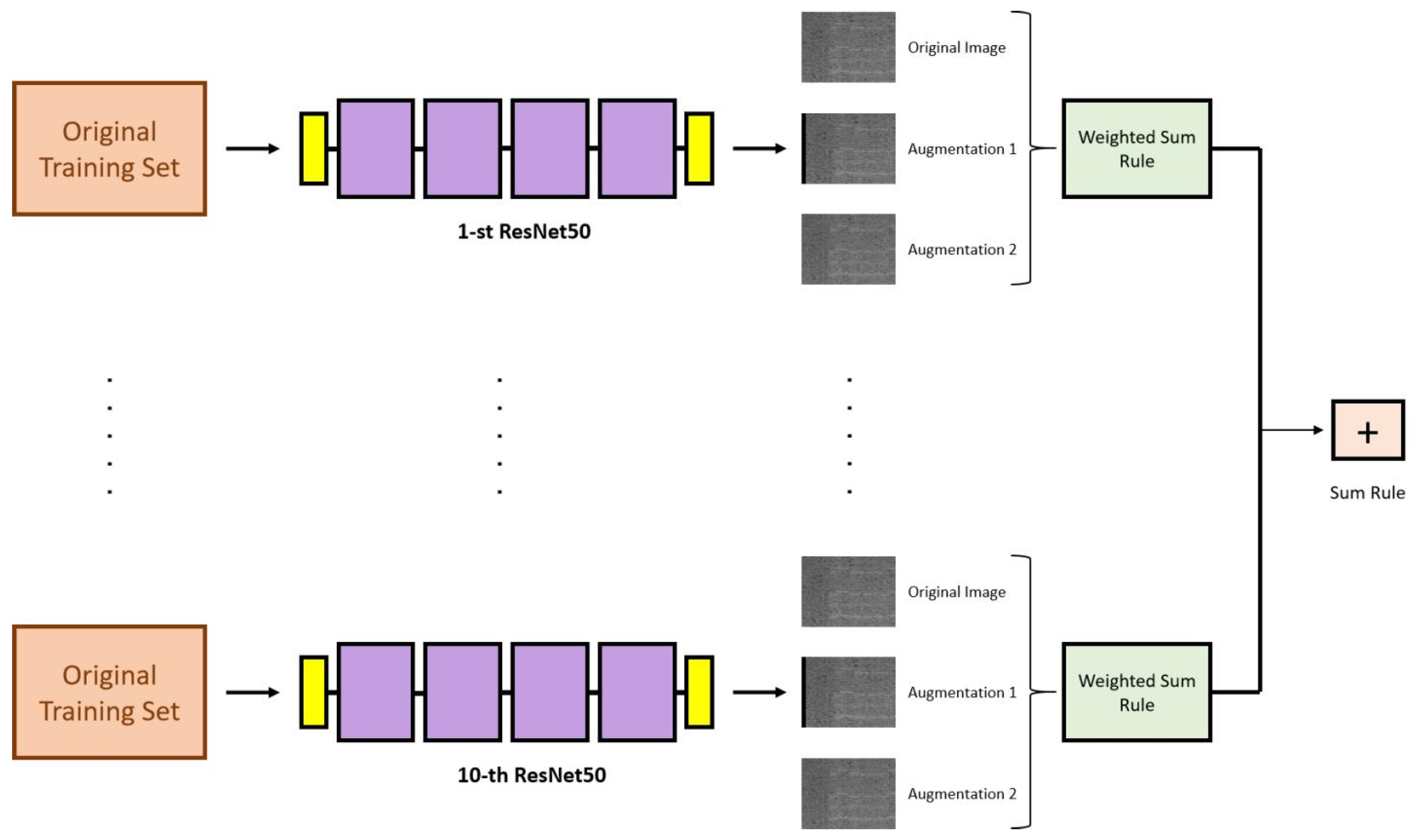
2.3. Proposed Approach

The approach proposed in this study is illustrated in Figure 1. Our method is based on the combination of ten ResNet50 networks. The data augmentation phase was applied only to the test set and not to the training set, since it is already a large set of spectrograms. The data augmentation methods were selected using the validation set. Moreover, by using the validation set, the weights of the weighted sum rule are fixed (see Section 2.3.2). As illustrated in Figure 1, for each image of the test set, we classified three images: the original and two created by the data augmentation methods. The scores of these three images were combined using the weighted sum rule (see Section 3 for details), where the weights were found using the validation set. The weighted sum rule is a machine learning approach that combines the predictions of multiple models, in which a factor weights the contribution of each model, here learned on the validation set. Altogether, we had ten ResNet50 networks (each obtained by simply reiterating training), which produced ten weighted sums. These ten scores (i.e., the output of the ten weighted sum rules, one for each network) were combined with the classic sum rule, obtaining the final score of the method.

In summary, we trained 10 resnet50 by simply tuning 10 times the ResNet50 network on the training dataset, then we used each of these 10 networks to classify the three images related to each pattern in the test set (original pattern and the two created by unsupervised data augmentation). For each network, we calculated the final score of each test pattern using the weighted sum rule, then these 10 scores (related to the 10 networks) were combined using the sum rule. These steps are described in more detail below.

2.3.1. ResNet50

ResNet50 is a convolutional neural network (CNN) architecture introduced by Microsoft Research in 2015 that belongs to a family of models called Residual Networks, or ResNets [37], which are widely used for various computer vision tasks, including image classification, object detection, and image segmentation. The key innovation of ResNet is the introduction of residual, or skip, connections for optimal gradient flow. ResNet enables the training of much deeper networks with improved performance by using skip connections. The name “ResNet50” signifies that this particular model has 50 layers.

The architecture of ResNet50 can be divided into several blocks. The input to the network is a 224 × 224 RGB image. The initial layer is a standard convolutional layer followed by a batch normalization layer and a ReLU activation function. This layer is followed by a max-pooling layer that reduces the spatial dimensions of the input. The main building blocks of ResNet50 are the residual blocks. Each residual block consists of a series of convolutional layers with batch normalization and ReLU activation. The output of these convolutional layers is added to the original input of the block through a skip connection. This addition operation allows the network to learn the residual information, i.e., the difference between the desired output and the input, which can be thought of as the “error” to be corrected.

ResNet50 contains several stacked residual blocks, with the number of blocks varying depending on the specific architecture. The model also includes bottleneck layers, which are 1 × 1 convolutional layers used to reduce the dimensionality of the feature maps, making the network more computationally efficient.

Towards the end of the network, a global average pooling layer spatially averages the feature maps, resulting in a fixed-length vector representation. This vector is fed into a fully connected layer with a softmax activation function, producing the final class probabilities.

Overall, ResNet50 is a powerful and influential CNN architecture that has significantly advanced the field of computer vision. Its use of residual connections has paved the way for the development of even deeper and more accurate neural networks, and it continues to serve as a benchmark for many state-of-the-art models in the field.

2.3.2. Validation Set Construction

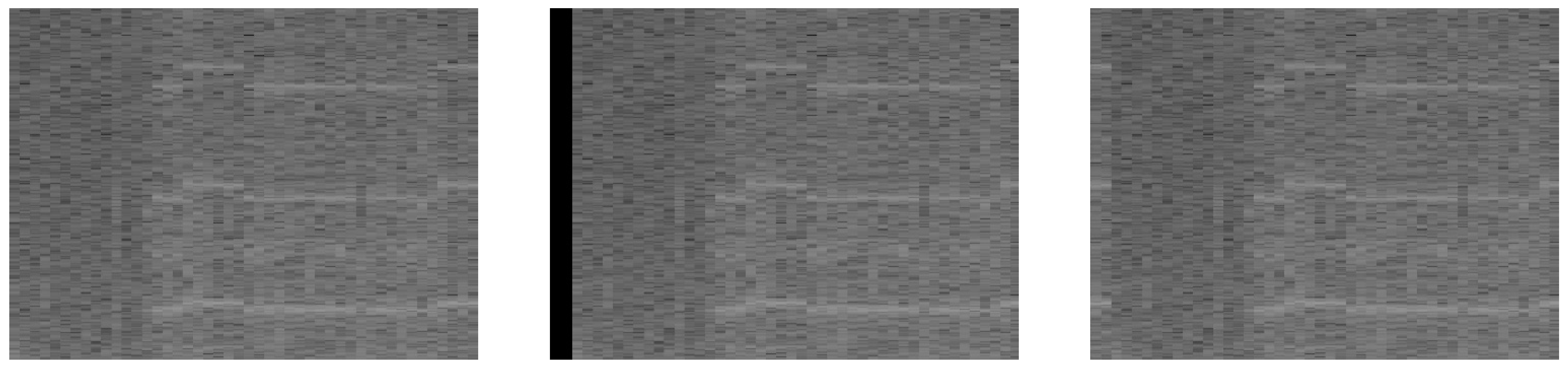
The original training and test sets in [28], as described in Section 2.1.2, were used in this study. However, unlike the original authors, we extracted a validation set from the training set using all the spectrograms related to the three-day recording period of 24 June to 26 June. The validation set was used to fix the parameters of the weights for combining the scores using the sum rule of the different augmented spectrograms created for each test pattern. Our testing set was composed of the original image and two augmented images. The data augmentation approaches are detailed in Section 2.3.3.

Using the validation set, we combined the following three spectrograms for each test pattern using the weighted sum rule:

• Original pattern;
• Random shift with black or wrap;
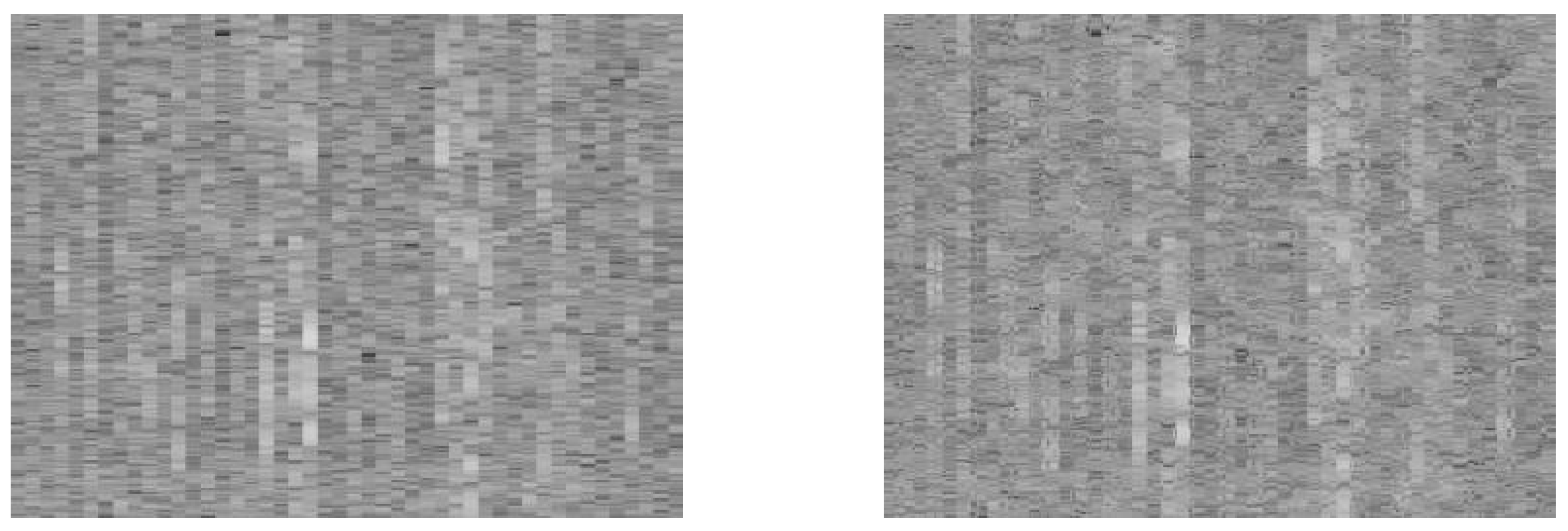
• Symmetric alternating diagonal shift.

2.3.3. Test Set Construction

The following two unsupervised data augmentation functions (see Figure 2 and Figure 3) were used to generate two images for each test image:

1

The Random shift with black or wrap (RS) augmentation function undertakes the task of randomly shifting the content of each image. The shift can be either to the left or right, determined by an equal probability of 50% for each direction. The shift’s magnitude falls within a specified shift width. Upon performing the shift, an empty space is created within the image. To handle this void, the function uses one of two strategies, each of which is selected with an equal chance of 50%. The first strategy is to fill the space with a black strip, and the second is to wrap the cut piece from the original image around to the other side, effectively reusing the displaced part of the image. In our tests, we utilized a shift_width randomly selected between 1 and 90.

2

The symmetric alternating diagonal shift (SA) augmentation function applies diagonal shifts to distinct square regions within each image. Specifically, the content of a selected square region is moved diagonally in the direction of the top-left corner. The subsequent square region undergoes an opposite shift, with its content displaced diagonally towards the bottom-right corner. The size of the square regions is chosen randomly within the specified minimum and maximum size range.

We tested many data augmentation methods. Due to space constraints, we only present the the methods that were selected based on the validation set.

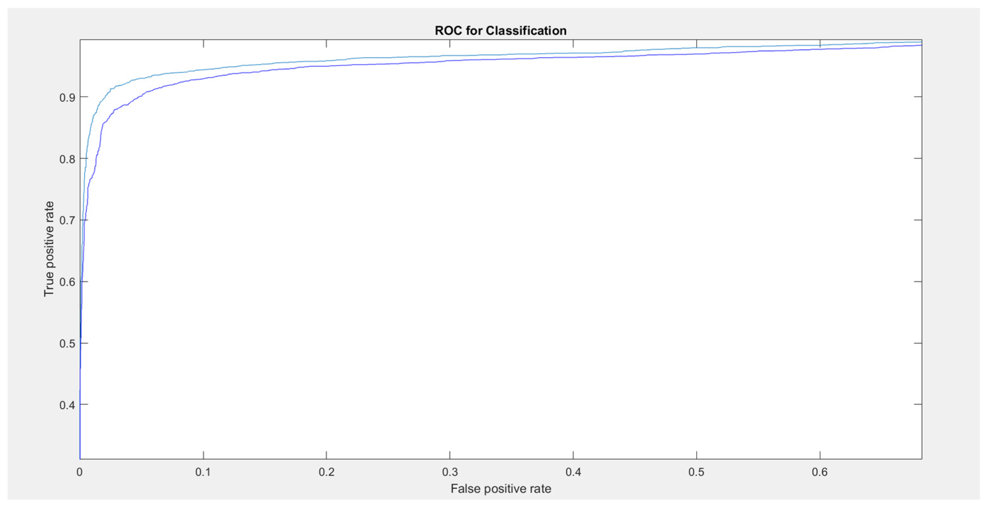
3. Experimental Results

The protocol used in our experiments mirrored that proposed in [28]. However, we used the validation set described in Section 2.3.2 to learn which data augmentation methods to apply and the weights of the weighted sum rule. After choosing the weights based on the validations set, we used the subdivision of the training and testing set described in [28]. We wish to stress that the validation set was extracted from the training set, so there was no overfitting on the test set. We gauged the performance of the model on the distinct test set by calculating the same performance indicators used in [28]. The true positive rate and the false positive rate was used to ascertain precision/recall. These metrics were used to generate the receiver operating characteristic (ROC) curves and evaluate the corresponding area under the ROC curve (AUC):

$$Precision=TP/\left(TP+FP\right)$$

(1)

$$Recall=TP/\left(TP+FN\right)$$

(2)

$$True Positive Rate=TP/\left(TP+FN\right);$$

(3)

where TP indicates true positives, TN indiates true negatives, FP indicates false positives, and FN indicates false negatives.

In

Table 1. Comparison (Area under the ROC curve) of baseline ResNet50(1) with the proposed augmented ensembles of ResNet50s (ResNet50(x)_DA (bold indicates best performance).

ResNets	AUC
ResNet50(1)	0.960
ResNet50(1)_DA	0.964
ResNet50(5)_DA	0.972
ResNet50(10)_DA	0.973

, we present a comparison between the baseline ResNet50 and the proposed data augmented ResNet50 (named ResNet50_DA). ResNet50(x)_DA indicates the combination of $x$ ResNet50_DA networks using the sum rule. Figure 4 reports the ROC curve for ResNet50(1) vs. ResNet50(10)_DA.

We acknowledge that the performance increase recorded in Table 1 may not appear high compared to the baseline. However, our results are interesting because many of the misclassified samples are unclassifiable by humans. Thus, we are likely already very close to the maximum performance ($AUC=1$ not obtainable). Furthermore, our results create a new baseline on an available dataset that can be repeated for testing other methods. The plot of the ROC curve in Figure 4 clearly shows that our proposed approach outperforms ResNet50(1). It is important to note that we obtained a true positive rate of 0.9 and a false positive rate of 0.02. Moreover, it is clear that the ResNet50(10)_DA improves ResNet50(1). The number of false positives of the standalone networks was more then two times the number of false positives of the ensemble.

In

Table 2. Comparison with the literature using four measures.

Method	Accuracy	AUC	Precision	Recall
Pamguard [14]	0.664	---	0.755	0.195
[28]	0.923	0.960	0.905	0.896
ResNet50(10)_DA	0.949	0.973	0.965	0.902

, we present a comparison between our proposed method and two other approaches using the same dataset with the same testing protocol, reporting a full set of performance indicators (accuracy, AUC, precision, and recall). Clearly, the proposed ensemble performed better than the methods reported in the literature, although with higher computational costs. We do not believe this is a problem, considering that the current computing power of GPUs and the developments expected in the coming years will reduce the considerations of such costs. For example, using a NVIDIA 1080, we were able to classify a batch of 100 spectrograms in ~0.3 s (considering a standalone ResNet50). Using a TitanRTX, we were able to classify a batch of 100 spectrograms in ~0.195 s (considering a standalone ResNet(50).

In

Table 3. Confusion matrices and Cohen’s kappa coefficient.

	Here		[28]		Pamguard [14]		Cohen’s Kappa
							Here	[28]	Pamguard [14]
	Noise	Whistle	Noise	Whistle	Noise	Whistle	0.8919	0.8383	0.1797
Noise	4124	88	3963	249	4044	168
Whistle	260	2397	277	2380	2139	518

, we present a report of the confusion matrix obtained by our proposed ensemble and the previous baseline on the same dataset. This test shows that the reliability of the proposed method reduces the number of false noise and false whistle classifications with respect to the previous baselines. In addition, Cohen’s kappa coefficient is also shown in the same table; this performance indicator also shows that the proposed ensemble outperformed the previous baseline.

In addition to the tests reported above, we conducted experiments in which the two data augmentation approaches selected on the validation set were applied to the whole training set. Due to the large size of the augmented training set, the training time increased to ~2100 min using a machine with a NVIDIA Titan X with 12 GB of ram. Increasing the size of the training set only slightly increased the performance. Once again, applying data augmentation to the test data using the weighted sum rule adopted in this paper resulted in better performance than using only the original test set. We obtained the following performance metrics:

1

Data augmentation applied to the training set, with the test set consisting of only the original images: AUC: 0.968; Accuracy: 0.940; Recall: 0.911 Precision: 0.931;

2

Data augmentation applied to both the training set and test set, with the proposed weighted sum rule used for the test set: AUC: 0.970; Accuracy: 0.941; Recall: 0.911; Precision: 0.934.

4. Conclusions

The surge in human activities in marine environments has led to an influx of boats and ships that emit powerful acoustic signals, often impacting areas larger than 20 square kilometers. The underwater noise from larger vessels can surpass 100 PSI, disturbing marine mammals’ hearing, navigation, and foraging abilities, particularly for coastal dolphins [38,39]. Therefore, the monitoring and preservation of marine ecosystems and wildlife is paramount. However, conventional monitoring technologies depend on detection methods that are less than ideal, thereby hindering our capacity to carry out extensive, long-term surveys. While automatic detection methods could significantly enhance our survey capabilities, their performance is typically subpar amidst high background noise levels.

In this paper, we illustrated how deep learning techniques involving data augmentation can identify dolphin whistles with remarkable accuracy, positioning them as a promising candidate for standardizing the automatic processing of underwater acoustic signals. We obtained state-of-the-art results and provided a training and test set for fair comparison. In terms of accuracy, we obtained a nearly 0.03 accuracy gain. The MATLAB/PyTorch source code used in this study is freely provided (https://github.com/LorisNanni/ accessed on 7 July 2023).

Despite the need for additional research to confirm the efficacy of such techniques across various marine environments and animal species, we are confident that deep learning will pave the way for developing and deploying economically feasible monitoring platforms. We hope that our new baseline will further the comparison of future deep learning techniques in this area.

Finally, we should stress the main cons of using this dataset as a benchmark: the training and test set were from the same region (Dolphin’s Reef in Eilat, Israel), and the samples were collected using the same acoustic recorder.

References

1. Halpern, B.S.; Frazier, M.; Afflerbach, J.; Lowndes, J.S.; Micheli, F.; O’hara, C.; Scarborough, C.; Selkoe, K.A. Recent pace of change in human impact on the world’s ocean. Sci. Rep. 2019, 9, 11609. [Google Scholar] [CrossRef] [PubMed] [Green Version]
2. Danovaro, R.; Carugati, L.; Berzano, M.; Cahill, A.E.; Carvalho, S.; Chenuil, A.; Corinaldesi, C.; Cristina, S.; David, R.; Dell’Anno, A.; et al. Implementing and Innovating Marine Monitoring Approaches for Assessing Marine Environmental Status. Front. Mar. Sci. 2016, 3, 213. [Google Scholar] [CrossRef]
3. Gibb, R.; Browning, E.; Glover-Kapfer, P.; Jones, K.E. Emerging opportunities and challenges for passive acoustics in ecological assessment and monitoring. Methods Ecol. Evol. 2019, 10, 169–185. [Google Scholar] [CrossRef] [Green Version]
4. Desjonquères, C.; Gifford, T.; Linke, S. Passive acoustic monitoring as a potential tool to survey animal and ecosystem processes in freshwater environments. Freshw. Biol. 2020, 65, 7–19. [Google Scholar] [CrossRef] [Green Version]
5. Macaulay, J.; Kingston, A.; Coram, A.; Oswald, M.; Swift, R.; Gillespie, D.; Northridge, S. Passive acoustic tracking of the three-dimensional movements and acoustic behaviour of toothed whales in close proximity to static nets. Methods Ecol. Evol. 2022, 13, 1250–1264. [Google Scholar] [CrossRef]
6. Wijers, M.; Loveridge, A.; Macdonald, D.W.; Markham, A. CARACAL: A versatile passive acoustic monitoring tool for wildlife research and conservation. Bioacoustics 2021, 30, 41–57. [Google Scholar] [CrossRef]
7. Ross, S.R.P.; O’Connell, D.P.; Deichmann, J.L.; Desjonquères, C.; Gasc, A.; Phillips, J.N.; Sethi, S.S.; Wood, C.M.; Burivalova, Z. Passive acoustic monitoring provides a fresh perspective on fundamental ecological questions. Funct. Ecol. 2023, 37, 959–975. [Google Scholar] [CrossRef]
8. Kowarski, K. Humpback Whale Singing Behaviour in the Western North Atlantic: From Methods for Analysing Passive Acoustic Monitoring Data to Understanding Humpback Whale Song Ontogeny. Ph.D. Thesis, Dalhousie University, Halifax, NS, Canada, 2020. [Google Scholar]
9. Arranz, P.; Miranda, D.; Gkikopoulou, K.C.; Cardona, A.; Alcazar, J.; de Soto, N.A.; Thomas, L.; Marques, T.A. Comparison of visual and passive acoustic estimates of beaked whale density off El Hierro, Canary Islands. J. Acoust. Soc. Am. 2023, 153, 2469. [Google Scholar] [CrossRef]
10. Lusseau, D. The emergent properties of a dolphin social network. Proc. R. Soc. B Boil. Sci. 2003, 270 (Suppl. 2), S186–S188. [Google Scholar] [CrossRef]
11. Lehnhoff, L.; Glotin, H.; Bernard, S.; Dabin, W.; Le Gall, Y.; Menut, E.; Meheust, E.; Peltier, H.; Pochat, A.; Pochat, K.; et al. Behavioural Responses of Common Dolphins Delphinus delphis to a Bio-Inspired Acoustic Device for Limiting Fishery By-Catch. Sustainability 2022, 14, 13186. [Google Scholar] [CrossRef]
12. Papale, E.; Fanizza, C.; Buscaino, G.; Ceraulo, M.; Cipriano, G.; Crugliano, R.; Grammauta, R.; Gregorietti, M.; Renò, V.; Ricci, P.; et al. The Social Role of Vocal Complexity in Striped Dolphins. Front. Mar. Sci. 2020, 7, 584301. [Google Scholar] [CrossRef]
13. Oswald, J.N.; Barlow, J.; Norris, T.F. Acoustic identification of nine delphinid species in the eastern tropical Pacific Ocean. Mar. Mammal Sci. 2003, 19, 20–37. [Google Scholar] [CrossRef] [Green Version]
14. Gillespie, D.; Caillat, M.; Gordon, J.; White, P. Automatic detection and classification of odontocete whistles. J. Acoust. Soc. Am. 2013, 134, 2427–2437. [Google Scholar] [CrossRef] [PubMed]
15. Serra, O.; Martins, F.; Padovese, L. Active contour-based detection of estuarine dolphin whistles in spectrogram images. Ecol. Informatics 2020, 55, 101036. [Google Scholar] [CrossRef]
16. Siddagangaiah, S.; Chen, C.-F.; Hu, W.-C.; Akamatsu, T.; McElligott, M.; Lammers, M.O.; Pieretti, N. Automatic detection of dolphin whistles and clicks based on entropy approach. Ecol. Indic. 2020, 117, 106559. [Google Scholar] [CrossRef]
17. Parada, P.P.; Cardenal-López, A. Using Gaussian mixture models to detect and classify dolphin whistles and pulses. J. Acoust. Soc. Am. 2014, 135, 3371–3380. [Google Scholar] [CrossRef] [PubMed]
18. Jarvis, S.; DiMarzio, N.; Morrissey, R.; Morretti, D. Automated classification of beaked whales and other small odontocetes in the tongue of the ocean, bahamas. In Proceedings of the OCEANS 2006, Boston, MA, USA, 18–21 September 2006. [Google Scholar]
19. Ferrer-I-Cancho, R.; McCowan, B. A Law of Word Meaning in Dolphin Whistle Types. Entropy 2009, 11, 688–701. [Google Scholar] [CrossRef] [Green Version]
20. Oswald, J.N.; Rankin, S.; Barlow, J.; Lammers, M.O. A tool for real-time acoustic species identification of delphinid whistles. J. Acoust. Soc. Am. 2007, 122, 587–595. [Google Scholar] [CrossRef] [Green Version]
21. Mouy, X.; Bahoura, M.; Simard, Y. Automatic recognition of fin and blue whale calls for real-time monitoring in the St. Lawrence. J. Acoust. Soc. Am. 2009, 126, 2918–2928. [Google Scholar] [CrossRef] [PubMed]
22. Usman, A.M.; Ogundile, O.O.; Versfeld, D.J.J. Review of Automatic Detection and Classification Techniques for Cetacean Vocalization. IEEE Access 2020, 8, 105181–105206. [Google Scholar] [CrossRef]
23. Abayomi-Alli, O.O.; Damaševičius, R.; Qazi, A.; Adedoyin-Olowe, M.; Misra, S. Data Augmentation and Deep Learning Methods in Sound Classification: A Systematic Review. Electronics 2022, 11, 3795. [Google Scholar] [CrossRef]
24. Testolin, A.; Diamant, R. Combining denoising autoencoders and dynamic programming for acoustic detection and tracking of underwater moving targets. Sensors 2020, 20, 2945. [Google Scholar] [CrossRef] [PubMed]
25. Jiang, J.-J.; Bu, L.-R.; Duan, F.-J.; Wang, X.-Q.; Liu, W.; Sun, Z.-B.; Li, C.-Y. Whistle detection and classification for whales based on convolutional neural networks. Appl. Acoust. 2019, 150, 169–178. [Google Scholar] [CrossRef]
26. Zhong, M.; Castellote, M.; Dodhia, R.; Ferres, J.L.; Keogh, M.; Brewer, A. Beluga whale acoustic signal classification using deep learning neural network models. J. Acoust. Soc. Am. 2020, 147, 1834–1841. [Google Scholar] [CrossRef] [PubMed]
27. Buchanan, C.; Bi, Y.; Xue, B.; Vennell, R.; Childerhouse, S.; Pine, M.K.; Briscoe, D.; Zhang, M. Deep convolutional neural networks for detecting dolphin echolocation clicks. In Proceedings of the 2021 36th International Conference on Image and Vision Computing New Zealand (IVCNZ), Tauranga, New Zealand, 9–10 December 2021. [Google Scholar]
28. Korkmaz, B.N.; Diamant, R.; Danino, G.; Testolin, A. Automated detection of dolphin whistles with convolutional networks and transfer learning. Front. Artif. Intell. 2023, 6, 1099022. [Google Scholar] [CrossRef] [PubMed]
29. Li, L.; Qiao, G.; Liu, S.; Qing, X.; Zhang, H.; Mazhar, S.; Niu, F. Automated classification of Tursiops aduncus whistles based on a depth-wise separable convolutional neural network and data augmentation. J. Acoust. Soc. Am. 2021, 150, 3861–3873. [Google Scholar] [CrossRef] [PubMed]
30. Li, P.; Liu, X.; Palmer, K.J.; Fleishman, E.; Gillespie, D.; Nosal, E.M.; Shiu, Y.; Klinck, H.; Cholewiak, D.; Helble, T.; et al. Learning deep models from synthetic data for extracting dolphin whistle contours. In Proceedings of the 2020 International Joint Conference on Neural Networks (IJCNN), Glasgow, UK, 19–24 July 2020. [Google Scholar]
31. Jin, C.; Kim, M.; Jang, S.; Paeng, D.-G. Semantic segmentation-based whistle extraction of Indo-Pacific Bottlenose Dolphin residing at the coast of Jeju island. Ecol. Indic. 2022, 137, 108792. [Google Scholar] [CrossRef]
32. Zhang, L.; Huang, H.-N.; Yin, L.; Li, B.-Q.; Wu, D.; Liu, H.-R.; Li, X.-F.; Xie, Y.-L. Dolphin vocal sound generation via deep WaveGAN. J. Electron. Sci. Technol. 2022, 20, 100171. [Google Scholar] [CrossRef]
33. Kershenbaum, A.; Sayigh, L.S.; Janik, V.M. The encoding of individual identity in dolphin signature whistles: How much information is needed? PLoS ONE 2013, 8, e77671. [Google Scholar] [CrossRef] [PubMed] [Green Version]
34. Padovese, B.; Frazao, F.; Kirsebom, O.S.; Matwin, S. Data augmentation for the classification of North Atlantic right whales upcalls. J. Acoust. Soc. Am. 2021, 149, 2520–2530. [Google Scholar] [CrossRef] [PubMed]
35. Tukey, J.W. Comparing Individual Means in the Analysis of Variance. Biometrics 1949, 5, 99–114. [Google Scholar] [CrossRef] [PubMed]
36. Jones, B.; Zapetis, M.; Samuelson, M.M.; Ridgway, S. Sounds produced by bottlenose dolphins (Tursiops): A review of the defining characteristics and acoustic criteria of the dolphin vocal repertoire. Bioacoustics 2020, 29, 399–440. [Google Scholar] [CrossRef]
37. He, K.; Zhang, X.; Ren, S.; Sun, J. Deep Residual Learning for Image Recognition. In Proceedings of the 2016 IEEE Conference on Computer Vision and Pattern Recognition (CVPR), Las Vegas, NV, USA, 27–30 June 2016; pp. 770–778. [Google Scholar]
38. Ketten, D.R. Underwater ears and the physiology of impacts: Comparative liability for hearing loss in sea turtles, birds, and mammals. Bioacoustics 2008, 17, 312–315. [Google Scholar] [CrossRef]
39. Erbe, C.; Marley, S.A.; Schoeman, R.P.; Smith, J.N.; Trigg, L.E.; Embling, C.B. The Effects of Ship Noise on Marine Mammals—A Review. Front. Mar. Sci. 2019, 6, 606. [Google Scholar] [CrossRef] [Green Version]
Figure 1. Proposed ensemble: for each image in the test set, we classified three images (the original and two augmented images) combined using the weighted sum rule.
Applsci 13 08029 g001
Figure 2. Spectrograms illustrating the RS method described in Section 2.3.3, with time on the x-axis and frequency in hertz on the y-axis. The left image showcases the original spectrogram. The center image presents the spectrogram after applying the random shift. The right image demonstrates the filled version of the spectrogram.
Applsci 13 08029 g002
Figure 3. Illustration of the SA method described in Section 2.3.3, with time on the x-axis and frequency in hertz on the y-axis. The left image showcases the original spectrogram. The right image presents the spectrogram after SA.
Applsci 13 08029 g003
Figure 4. ROC curve (ratios of the true positives on the y-axis and false positives on the x-axis). The light blue represents our proposed ensemble, and the dark blue represents ResNet50(1), a single network.
Applsci 13 08029 g004