Switching Control of Closed-Loop Supply Chain Systems with Markov Jump Parameters

Abstract

The switching system model of a closed-loop supply chain with Markov jump parameters is established. The system is modeled as a switching system with Markov jump parameters, taking into account the uncertainties of the process and the inventory decay factors. The Markov switching idea is applied to the controller design and performance analysis of the system to effectively suppress the bullwhip effect while ensuring the stability of the closed-loop supply chain system. Simulation examples are presented to illustrate the validity of the results obtained.

1. Introduction

With the development of productivity and the growing awareness of resource use and environmental protection, research on closed-loop supply chains has attracted more and more attention [1,2,3,4]. In recent years, research on manufacturing and remanufacturing systems has attracted extensive attention. Industry practice shows that remanufacturing in closed-loop supply chains not only helps to reduce resource consumption but also helps to save costs and improve competitive advantages [5]. Because remanufacturing is profitable and environmentally efficient, many enterprises have established their own recycling and remanufacturing systems and voluntarily carried out remanufacturing activities, such as IBM, HP, BMW, Ford, Apple, Kodak, Xerox, Caterpillar, etc. [6,7]. Therefore, consideration of the remanufacturing link in closed-loop supply chain systems [8,9] is being paid more attention. Ref. [10] considers the supply chain model with a product remanufacturing link, Ref. [11] investigates the problem of effective channel design for closed-loop supply chain systems, and Ref. [12] determines productivity, remanufacturing rates, and disposal rates through a cost optimization approach. Ref. [13] applied the Pontryagin maximum value principle [14] and studied a linear model for optimizing production, remanufacturing, and abandonment strategies. In addition, a number of scholars have started to focus on closed-loop supply chain production–inventory control systems: Ref. [15] used optimal control ideas to study the dynamic capacity planning problem of closed-loop supply chain remanufacturing systems; Ref. [16] applied the ideas of game theory to the network equilibrium problem of closed-loop supply chain systems; and Ref. [17,18] applied fuzzy logic ideas to study the product recovery strategy of closed-loop supply chains.

It is worth noting that the above-mentioned literature mainly focuses on the static environment, while it is obvious that the static model is not sufficient to portray the dynamic characteristics of closed-loop supply chain systems such as demand fluctuation, production lead time, sales forecast, etc. Therefore, supply chain analysis based on a dynamic model has achieved some results [19,20,21,22], among which, modeling the closed-loop supply chain as a kind of dynamic behavior of switching system has attracted great attention from many scholars [23,24], and it is generally believed that a switching system with Markov jump parameters is an appropriate model to describe the closed-loop supply chain system. The robust production and maintenance scheduling problem is described in [19] as a minimax statistical control problem. The machine state process is modeled as a finite-state Markov chain whose generator depends on the rate of aging, productivity, and maintenance, modeling the demand rate as an unknown interference process. Ref. [25] studies the control problem of a closed-loop supply chain switching system with Markov jump parameters. Aiming at the uncertainty problem in the process of remanufacturing, based on the input lag control strategy, the Markov switching idea is applied to the controller design and performance analysis of the system. However, modeling the production–inventory model of a closed-loop supply chain system as a switching system with Markov jump parameters has rarely been reported [26], which is one of the main motivations for this study.

The bullwhip effect is the phenomenon of demand fluctuation amplification in supply chain and is the most important performance indicator in supply chain operations [27,28,29]. The bullwhip effect exists in a supply chain and more extensive ERP, e-commerce, and other management systems, including modern logistics operation. It has important theoretical significance and wide application prospect to study bullwhip effect of a closed-loop supply chain system with a robust $H_{\infty }$ control method.

This paper studies the closed-loop supply chain production–inventory system of remanufacturing. Considering the inventory decay factor, the corresponding subsystems are determined according to the different inventory status, and the switching system with Markov jump parameters is established. Meanwhile, the $H_{\infty }$ control method [30] in robust control is applied. In the form of LMI, sufficient conditions are given to ensure the stability of the system and have $H_{\infty }$ performance in suppressing the bullwhip effect. Finally, a numerical example of scrap recycling in a domestic iron and steel enterprise is used to illustrate the validity of the results obtained.

2. Closed-Loop Supply Chain Switching System Modeling

This paper considers the control problem of a closed-loop supply chain system based on remanufacturing. The model assumes that a manufacturer produces a product, and at the same time, the manufacturer retrieves that product from the market for remanufacturing. This paper assumes that the quality standard of the remanufactured goods can meet the standard of the new products. This paper mainly considers the problem of inventory management. Manufactured and remanufactured goods are stored in the usable goods warehouse, and used goods recovered from the market are stored in the recycled goods warehouse. $x_1\left(k\right)$ and $x_2\left(k\right)$ represent the inventory levels of the available commodity warehouse and the recycled commodity warehouse and are the state vector of the system. $u_1\left(k\right)$ and $u_2\left(k\right)$ represent the manufacturing rate of the manufacturing equipment and the recycling rate of the used goods at the moment, respectively. For the system model, we have the following assumptions.

Assumption A1.

Assume that all products are recyclable and that the manufacturer is the only determinant of the amount of product to be recycled, i.e., that there are sufficient products on the market to meet the demand for recycling and that the manufacturer only needs to recycle the amount of product it needs.

Assumption A2.

The market demand $d\left(k\right)$ is the sum of the constant $\overline{d}$ and the perturbation $\omega \left(k\right)$, i.e.,

$$d\left(k\right)=\overline{d}+\omega \left(k\right)$$

Note 1.

For the sake of generality, it is assumed that the perturbations $\omega \left(k\right)$ follow a normal distribution or are sinusoidal functions.

Assumption A3.

Recycled products are disposed of in two ways, remanufacturing and disposal, so that α$(0\le \alpha \le 1)$ represents the remanufacturing rate, β$(0\le \beta \le 1)$ the disposal rate, and α and β are uncertain parameters; $0<\alpha +\beta \le 1$ is assumed in this paper.

Assumption A4.

The value of the products in the warehouse decreases over time. ${\rho }_1$ and ${\rho }_2$ represent the decay rates of the available and recovered warehouses, respectively.

The closed-loop supply chain system considered in this paper have inventory levels as the state variable.

First, for the available commodity warehouse, when $0<x_1\left(k\right)<c_{max}^1$, the system is given by the following equation

$$\begin{array}{c}\hfill x_1(k+1)=(1-{\rho }_1)x_1\left(k\right)+\alpha x_2\left(k\right)+u_1\left(k\right)-d\left(k\right)\end{array}$$

(1)

where $c_{max}^1$ is the maximum capacity of the available warehouse.

It should be noted that when $x_1\left(k\right)\le 0$ indicates that there are no items in the warehouse that can be used to meet the order demand, which also results in a stock-out phenomenon. At this point, the production–inventory model can be described as

$$\begin{array}{c}\hfill x_1(k+1)=x_1\left(k\right)+\alpha x_2\left(k\right)+u_1\left(k\right)-d\left(k\right)\end{array}$$

(2)

Similarly, for the recycled goods inventory, let $c_{max}^2$ be the maximum capacity of the recycled goods warehouse; when $0<x_2\left(k\right)<c_{max}^2$, the system can be represented as

$$\begin{array}{c}\hfill x_2(k+1)=(1-{\rho }_2)x_2\left(k\right)-\alpha x_2\left(k\right)-\beta x_2\left(k\right)+u_2\left(k\right)\end{array}$$

(3)

When $x_2\left(k\right)\le 0$ is used, the system can be described as

$$\begin{array}{c}\hfill x_2(k+1)=x_2\left(k\right)+u_2\left(k\right)\end{array}$$

(4)

Let $y\left(k\right)$ be the operating cost of the system, then

$$\begin{array}{c}\hfill y\left(k\right)=(C+\Delta C)x\left(k\right)\end{array}$$

(5)

where $C=\left[\begin{array}{cc}{C}_{h1}& 0\\ 0& C_{h2}\end{array}\right]$, $\Delta C=\left[\begin{array}{cc}0& c_r\alpha +c_0\beta \end{array}\right]$, the parameters are as follows: $c_{h1}$ is the cost of useful inventory, $c_{h2}$ is the cost of remanufactured inventory, $c_r$ is the cost of remanufactured product, and $c_0$ is the cost of discard (all deterministic parameters).

Note 2.

The total closed-loop supply chain cost is determined by the cost of useful inventory, the cost of remanufactured inventory, the cost of remanufactured products, and the cost of waste disposal.

In order to establish a closed-loop supply chain production–inventory switching system model, let $x\left(k\right)={\left[\begin{array}{cc}{x}_1^T\left(k\right)& x_2^T\left(k\right)\end{array}\right]}^T$; considering Equations (1) and (3), the following closed-loop supply chain model can be obtained:

$$\begin{array}{c}\hfill \left\{\begin{array}{c}x(k+1)=(A_1+\Delta A_1)x\left(k\right)+B_{1}u\left(k\right)+b+B_2\omega \left(k\right)\hfill \\ y\left(k\right)=(C+\Delta C)x\left(k\right)\hfill \end{array}\right.\end{array}$$

(6)

where

$A_1=\left[\begin{array}{cc}1-{\rho }_1& 0\\ 0& 1-{\rho }_2\end{array}\right]$, $\Delta A_1=\left[\begin{array}{cc}0& \alpha \\ 0& -\alpha -\beta \end{array}\right]$, $b=\left[\begin{array}{c}-\overline{d}\\ 0\end{array}\right]$

$B_1=\left[\begin{array}{cc}1& 0\\ 0& 1\end{array}\right]$, $B_2=\left[\begin{array}{cc}-1& 0\\ 0& 0\end{array}\right]$, $u\left(k\right)=\left[\begin{array}{c}{u}_1\left(k\right)\\ u_2\left(k\right)\end{array}\right]$

Considering Equations (1) and (4), the supply chain model of the closed-loop system is as follows:

$$\begin{array}{c}\hfill \left\{\begin{array}{c}x(k+1)=(A_2+\Delta A_2)x\left(k\right)+B_{1}u\left(k\right)+b+B_2\omega \left(k\right)\hfill \\ y\left(k\right)=(C+\Delta C)x\left(k\right)\hfill \end{array}\right.\end{array}$$

(7)

where

$$A_2=\left[\begin{array}{cc}1-{\rho }_1& 0\\ 0& 1\end{array}\right],\Delta A_2=\left[\begin{array}{cc}0& \alpha \\ 0& 0\end{array}\right].$$

Similarly, combining Equation (2) with Equation (3), the following closed-loop supply chain system can be obtained:

$$\begin{array}{c}\hfill \left\{\begin{array}{c}x(k+1)=(A_3+\Delta A_3)x\left(k\right)+B_{1}u\left(k\right)+b+B_2\omega \left(k\right)\hfill \\ y\left(k\right)=(C+\Delta C)x\left(k\right)\hfill \end{array}\right.\end{array}$$

(8)

where

$$A_3=\left[\begin{array}{cc}1& 0\\ 0& 1-{\rho }_2\end{array}\right],\Delta A_3=\left[\begin{array}{cc}0& \alpha \\ 0& -\alpha -\beta \end{array}\right]$$

Finally, considering Equations (2) and (4), the following closed-loop supply chain system is obtained:

$$\begin{array}{c}\hfill \left\{\begin{array}{c}x(k+1)=(A_4+\Delta A_4)x\left(k\right)+B_{1}u\left(k\right)+b+B_2\omega \left(k\right)\hfill \\ y\left(k\right)=(C+\Delta C)x\left(k\right)\hfill \end{array}\right.\end{array}$$

(9)

where

$$A_4=\left[\begin{array}{cc}1& 0\\ 0& 1\end{array}\right],\Delta A_4=\left[\begin{array}{cc}0& \alpha \\ 0& 0\end{array}\right]$$

Suppose that the switch between the 4 subsystems is determined by the Markov process $\left\{\sigma \left(k\right),k\ge 0\right\}$ and that the transfer probabilities of $P={\left[P_{ij}\right]}_{(i,j\in S)}$, $\left\{\sigma \left(k\right),k\ge 0\right\}$ satisfy

$$\begin{array}{c}\hfill P\left[\left.\sigma (k+1)=j\right|\sigma \left(k\right)=i\right]=P_{ij},\forall i,j\in S\end{array}$$

(10)

and meet $P_{ij}\ge 0$, ${\displaystyle \sum _{j=1}^4}{P}_{ij}=1$.

The closed-loop supply chain system can be rewritten as a switching control system as follows:

$$\begin{array}{c}\hfill \left\{\begin{array}{c}x(k+1)=(A_{\sigma \left(k\right)}+\Delta A_{\sigma \left(k\right)})x\left(k\right)+B_{1}u\left(k\right)+b+B_2\omega \left(k\right)\hfill \\ y\left(k\right)=(C+\Delta C)x\left(k\right)\hfill \end{array}\right.\end{array}$$

(11)

where $\Delta A_i$, $\Delta C$ are uncertain matrices. Suppose it satisfies $\Delta A_i=H_{ai}{F}_{ai}{E}_{ai}$, where $F_{ai}$ is unknown matrices, and satisfies

$$\begin{array}{c}\hfill F_{ai}^T{F}_{ai}\le I,F_{ci}^T{F}_{ci}\le I.\end{array}$$

(12)

$H_{ai}$, $E_{ai}$, $H_{ci}$, and $E_{ci}$ are known matrices. In the following, $\Delta A_i$, $\Delta C$ is treated in that form, when $i=1,3$, $\Delta A_i=H_{ai}{F}_{ai}{E}_{ai}$, where

$$H_{ai}=\left[\begin{array}{cc}1& 0\\ 0& 1\end{array}\right],E_{ai}=\left[\begin{array}{cc}0& 1\\ 0& -1\end{array}\right],F_{ai}=\left[\begin{array}{cc}\alpha & 0\\ 0& \alpha +\beta \end{array}\right]$$

When $i=2,4$, $\Delta A_i=H_{ai}{F}_{ai}{E}_{ai}$, where

$$H_{ai}=\left[\begin{array}{cc}1& 0\\ 0& 0\end{array}\right],E_{ai}=\left[\begin{array}{cc}1& 0\\ 0& 1\end{array}\right]$$

$\Delta C=H_c{F}_c{E}_c$, where

$$H_c=\left[\begin{array}{cc}{c}_r& 0\\ 0& c_0\end{array}\right],F_c=\left[\begin{array}{cc}\alpha & 0\\ 0& \beta \end{array}\right],E_c=\left[\begin{array}{cc}1& 0\\ 0& 1\end{array}\right]$$

Note 3.

The bullwhip effect is the most significant performance indicator of a closed-loop supply chain analysis, which generates production control and recovery remanufacturing control through inventory levels $u\left(k\right)$, suppressing the perturbations of uncertain system demand $\omega \left(k\right)$, thereby minimizing the system operating costs $y\left(k\right)$, and this level of suppression can be described by the following equation:

$$\begin{array}{c}\hfill \frac{{∥y∥}_2}{{∥\omega ∥}_2}\le \gamma \end{array}$$

(13)

The smaller the $\gamma$, the better the performance of the system, and it is easy to see that Equation (13) is precisely the condition for the level of disturbance suppression in the $H_{\infty }$ control to satisfy the gain of $l_2$. In essence, the study of the suppression of the bullwhip effect in supply chain systems can be incorporated into the framework of the study of $H_{\infty }$ control.

Note 4.

This paper uses the idea of robust control to study the control problem of $H_{\infty }$ for switching systems with Markov jump parameters. Assumption (12) is a common assumption condition in robust control.

In a closed-loop supply chain system, the following state feedback control law is designed.

$$\begin{array}{c}\hfill u\left(k\right)=\widehat{b}+K_{\sigma \left(k\right)}x\left(k\right)\end{array}$$

(14)

The closed-loop supply chain switching system can be described as follows:

$$\begin{array}{c}\hfill \left\{\begin{array}{c}x(k+1)=(A_{\sigma \left(k\right)}+\Delta A_{\sigma \left(k\right)}+B_1{K}_{\sigma \left(k\right)})x\left(k\right)+B_2\omega \left(k\right)\hfill \\ y\left(k\right)=(C+\Delta C)x\left(k\right)\hfill \end{array}\right.\end{array}$$

(15)

The initial conditions of system (15) are given as follows:

$$\begin{array}{c}\hfill x\left(0\right)=x_0\end{array}$$

(16)

The objective of this paper is described as follows: to establish a switching system for a closed-loop supply chain with Markov jump parameters, on this basis, design a robust $H_{\infty }$ controller to make the closed-loop supply chain system with remanufacturing and abandonment stable under the condition of satisfying $H_{\infty }$ performance.

3. Stability Analysis and Controller Design

In this section, we give sufficient conditions for the mean square exponential stability of closed-loop supply chain systems with Markov jump parameters and give the design method of the state feedback control law.

The following lemma is used in this paper.

Lemma 1

([26]). Given matrices of appropriate dimensions $G=G^T$, H, E, for all matrices F satisfying $F^{T}F\le I$, such that, the following inequality holds:

$$G+HFE+E^T{F}^T{H}^T<0$$

Then, there exists the scalar $\epsilon >0$, such that the following inequality holds:

$$G+\epsilon H{H}^T+{\epsilon }^{-1}{E}^{T}E<0$$

Lemma 2

([31]). (Suhur’s Complementary Lemma) For a given symmetric matrix $R=\left[\begin{array}{cc}{R}_{11}& R_{12}\\ R_{12}^T& R_{22}\end{array}\right]$, where $R_{11}$ is $r\times r$ dimensional, the following three conditions are equivalent

(1) 

$R<0$.

(2) 

$R_{11}<0$, $R_{22}-R_{12}^T{R}_{11}^{-1}{R}_{12}<0$.

(3) 

$R_{22}<0$, $R_{11}-R_{12}{R}_{22}^{-1}{R}_{12}^T<0$.

In the following, we consider the following nominal system, i.e., the stability and robust $H_{\infty }$ control of the system in the case of $\Delta A_{\sigma \left(k\right)}\equiv 0$, $\Delta C_{\sigma \left(k\right)}\equiv 0$, with the nominal system modeled as

$$\begin{array}{c}\hfill \left\{\begin{array}{c}x(k+1)=(A_{\sigma \left(k\right)}+B_1{K}_{\sigma \left(k\right)})x\left(k\right)+B_2\omega \left(k\right)\hfill \\ y\left(k\right)=Cx\left(k\right)\hfill \end{array}\right.\end{array}$$

(17)

We begin by introducing the following two definitions:

Definition 1

([32]). For any initial condition $(x_0,0)$, if there exist constants α and λ such that

$$E\left\{{∥x\left(k\right)∥}^2\right\}\le \alpha e^{-\lambda k}{∥x_0∥}^2,k\to \infty$$

holds, the system (15) is said to be mean square exponentially stable.

Definition 2

([32]). For any disturbance initial condition level $\omega \left(t\right)\in l_2$, the system (15) is called mean square exponentially stable and has a dry disturbance suppression level γ if the system mean square index is stable and satisfies the constant ${∥y\left(k\right)∥}_2\le \gamma {∥\omega \left(k\right)∥}_2$, where ${∥y\left(k\right)∥}_2={\left[{\displaystyle \sum _{k=0}^{\infty }}E\left[y^T\left(k\right)y\left(k\right)\right]\right]}^{\frac{1}{2}}$.

The main results are given below.

Theorem 1.

The closed-loop supply chain system (17) with Markov jump parameters $\left\{\sigma \left(k\right),k\ge 0\right\}$ and state transition probability matrix satisfying condition (10) is exponentially stable with mean square and interference suppression level γ if, for a given positive constant λ, there exists a set of symmetric positive definite matrices $P_i$,$i\in S$, such that the following optimization problem can be solved:

$$\begin{array}{c}min\gamma \hfill \\ S.t\hfill \end{array}$$

$$\begin{array}{c}\hfill {\Sigma }_{i1}=\left[\begin{array}{cc}{(A_i+B_1{K}_i)}^T{G}_i(A_i+B_1{K}_i)+e^{-\lambda }{C}^{T}C-e^{-\lambda }{P}_i& {(A_i+B_1{K}_i)}^T{G}_i{B}_2\\ \ast & B_2^T{G}_i{B}_2-e^{-\lambda }{\gamma }^{2}I\end{array}\right]<0.\end{array}$$

(18)

where $G_i=\sum _{j=1}^4{p}_{ij}{P}_j$.

Proof. 

We first consider the system at $\omega \left(k\right)=0$. Additionally, by Schur’s complementary lemma, if Equation (18) holds, then

$${\Sigma }_{i0}={(A_i+B_1{K}_i)}^T{G}_i(A_i+B_1{K}_i)-e^{-\lambda }{P}_i<0.$$

Construct the following Lyapunov functional:

$$V(x_k,k)=x^T\left(k\right)P_{\sigma \left(k\right)}x\left(k\right)$$

For ease of writing, the matrix $A_{\sigma \left(k\right)}$ in the modal $\sigma \left(k\right)=i$ is denoted by $A_i$, and the rest of the matrices are denoted similarly. $F_n=\left\{\begin{array}{ccc}x\left(0\right),& \cdots ,& x\left(n\right)\end{array}\right\}$, $\forall n\ge 0$.

Considering the Markov property, a calculation based on conditional expectations readily yields

$$\begin{array}{c}E\left\{\left.V(k+1)\right|F_k\right\}-e^{-\lambda }V\left(k\right)\hfill \\ =x^T\left(k\right)({(A_i+B_1{K}_i)}^T{G}_i(A_i+B_1{K}_i)-e^{-\lambda }{P}_i)x\left(k\right)\hfill \\ =x^T\left(k\right){\Sigma }_{i0}x\left(k\right).\hfill \end{array}$$

We therefore have

$$E\left\{\left.V\left(x\right(k+1),k+1)\right|F_k\right\}-e^{-\lambda }V(x_k,k)\le -{\lambda }_{min}(-{\Sigma }_{i0}^{})x^T\left(k\right)x\left(k\right)\le -\beta x^T\left(k\right)x\left(k\right)$$

where ${\lambda }_{min}(-{\Sigma }_{i0}^{})$ denotes the smallest eigenvalue of $-{\Sigma }_{i0}^{}$ when $\sigma \left(k\right)\in S$, $\beta =inf\left\{{\lambda }_{min}(-{\Sigma }_{i0}^{})\right\}$. For any $K\ge 1$, there is

$$E\left\{V(k+1),K+1\right\}-e^{-\lambda k}E\left\{V(x_0,0\right\}=-\beta \sum _{k=0}^{K}E\left[x^T\left(k\right)x\left(k\right)\right]$$

and then by

$$\sum _{k=0}^{K}E\left[x^T\left(k\right)x\left(k\right)\right]\le \frac{1}{\beta }\left[e^{-\lambda }E\left\{V(x_0,0)\right\}-E\left\{V(x_{K+1},K+1\right\}\right]\le \frac{1}{\beta }{e}^{-\lambda k}E\left\{V(x_0,0)\right\}$$

It is possible to obtain

$$\sum _{k=0}^{\infty }E\left[x^T\left(k\right)x\left(k\right)\right]\le \frac{1}{\beta }{e}^{-\lambda k}E\left\{V(x_0,0)\right\}$$

Therefore, the system (17) mean square index is stable when $\omega \left(k\right)=0$. □

The following shows that the system satisfies $y^T\left(k\right)y\left(k\right)\le {\gamma }^2{\omega }^T\left(k\right)\omega \left(k\right)$, when $\omega \left(k\right)\ne 0$, under zero initial conditions. Define the following performance metrics.

$$J=E\left[\sum _{k=0}^N\left.\left[e^{-\lambda }{y}^T\left(k\right)y\left(k\right)-{\gamma }^2{\omega }^T\left(k\right)\omega \left(k\right)\right]\right|x_0,\sigma \left(0\right)\right]$$

From the zero initial condition, $V(x_0,0)=0$, $V\left(x\right(N+1\left)\right)\ge 0$, then

$$\begin{array}{c}J=E\{{\displaystyle \sum _{k=0}^N}{e}^{-\lambda }[y^T\left(k\right)y\left(k\right)-{\gamma }^2{\omega }^T\left(k\right)\omega \left(k\right)-V\left(x\left(k\right)\right)\hfill \\ +V\left(x\right(k+1\left)\right)+V\left(x\right(0\left)\right)-V\left(x\right(N+1\left)\right)\left]\right\}\hfill \\ \le {\displaystyle \sum _{k=0}^N}\left\{e^{-\lambda }{y}^T\left(k\right)y\left(k\right)-e^{-\lambda }{\gamma }^2{\omega }^T\left(k\right)\omega \left(k\right)+E\left[V(x(k+1)-e^{-\lambda }V(x\left(k\right)\right]\right\}\hfill \\ ={\displaystyle \sum _{k=0}^N}\left\{e^{-\lambda }{x}^T\left(k\right)C^{T}Cx\left(k\right)-e^{-\lambda }{\gamma }^2{\omega }^T\left(k\right)\omega \left(k\right)\right\}\hfill \\ \\ +x^T\left(k\right)({(A_i+B_1{K}_i)}^T{G}_i(A_i+B_1{K}_i)-e^{-\lambda }{P}_i)x\left(k\right)\hfill \\ \\ +{\omega }^T\left(k\right){B_2}^T{G}_i{B}_2\omega \left(k\right)+2x^T\left(k\right){(A_i+B_{1}K)}^T{G}_i{B}_2\omega \left(k\right)\hfill \\ \\ ={\xi }^T\left(k\right){\Sigma }_{i1}\xi \left(k\right)\hfill \end{array}$$

where

$$\xi \left(k\right)={\left[\begin{array}{cc}{x}^T\left(k\right)& {\omega }^T\left(k\right)\end{array}\right]}^T$$

From the theorem, if Equation (18) holds, then $J<0$.

Note 5.

The condition in Theorem 1 is not linear matrix inequality, because it contains the coupling term of the product of the controller gain matrix $K_i$ and the Lyapunov functional matrix. Therefore, Theorem 1 is just the result of the mean square stability of the system in theory and has no practical operational significance. The gain matrix $K_i$ of the controller can be obtained only by converting Equation (18) into linear matrix inequalities through appropriate matrix transformation.

Theorem 2.

The closed-loop supply chain system (17) with Markov jump parameter $\left\{\sigma \left(k\right),k\ge 0\right\}$ and state transition probability matrix satisfying condition (10) is mean square exponential stable and has disturbance suppression level γ. If for a given positive constant λ, there exists a set of symmetric positive definite matrices $X_i$, $Y_i$, $i\in S$, such that the following optimization problem can be solved, and if the following problem is feasible, the state feedback controller $K_i=Y_i{X_i}^{-1}$:

$$\begin{array}{c}\hfill {\Sigma }_{i2}=\left[\begin{array}{cccc}-e^{-\lambda }{X}_i& 0& {(A_i{X}_i+B_1{Y}_i)}^T{W}_i& X_i{C}^T\\ \ast & -e^{-\lambda }{\gamma }^{2}I& B_2^T{W}_i& 0\\ \ast & \ast & -\chi & 0\\ \ast & \ast & \ast & -e^{-\lambda }I\end{array}\right]<0.\end{array}$$

(19)

Proof. 

Let

$$W_i=\left(\begin{array}{cccc}\sqrt{p_{i1}}I& \sqrt{p_{i2}}I& \sqrt{p_{i3}}I& \sqrt{p_{i4}}I\end{array}\right),\chi =diag\left\{\begin{array}{cccc}{X}_1& X_2& X_3& X_4\end{array}\right\}$$

then

$$G_i=W_i\mathcal{P}{W}_i^T,\mathcal{P}=diag\left\{\begin{array}{cccc}{P}_1& P_2& P_3& P_4\end{array}\right\}$$

It is clear that

$$\begin{array}{cc}\hfill {\Sigma }_{i1}& =\left[\begin{array}{cc}{e}^{-\lambda }{C}^{T}C-e^{-\lambda }{P}_i& 0\\ 0& -e^{-\lambda }{\gamma }^{2}I\end{array}\right]\hfill \\ & +\left[\begin{array}{c}{(A_i+B_1{K}_i)}^T{W}_i\\ B_2^T{W}_i\end{array}\right]\mathcal{P}\left[\begin{array}{cc}{W}_i^T(A_i+B_1{K}_i)& B_2\end{array}\right]\hfill \end{array}$$

(20)

By Schur’s complementary lemma, the above equation is equivalent to

$$\begin{array}{c}\hfill \left[\begin{array}{cccc}-e^{-\lambda }{P}_i& 0& {(A_i+B_1{K}_i)}^T{W}_i& C^T\\ \ast & -e^{-\lambda }{\gamma }^{2}I& B_2^T{W}_i& 0\\ \ast & \ast & -{\mathcal{P}}^{-1}& 0\\ \ast & \ast & \ast & -e^{-\lambda }I\end{array}\right]<0\end{array}$$

(21)

The above equation is multiplied by $diag\left\{\begin{array}{cccc}{X}_i& I& I& I\end{array}\right\}$ and its transpose, $K_i{X}_i=Y_i$, on the left and right sides, respectively, to obtain Equation (19). □

In the following, we consider the uncertainty of the system due to the recycling remanufacturing rate and give sufficient conditions for the closed-loop supply chain system (15) to be exponentially stable in mean square and have a disturbance rejection level of $\gamma$ based on the idea of handling uncertainty in robust control thinking.

Theorem 3.

The closed-loop supply chain system (15) with Markov jump parameter $\left\{\sigma \left(k\right),k\ge 0\right\}$ and state transition probability matrix satisfying condition (10) is exponentially stable with mean square and interference suppression level γ. If for a given positive constant λ, there is a set of symmetric positive definite matrix $X_i$, $Y_i$, and parameter ${\epsilon }_{ai}$, ${\epsilon }_c$, which makes the following optimization problem solvable, and if the following problem is feasible, the state feedback controller $K_i=Y_i{X_i}^{-1}$.

$$\begin{array}{c}\hfill \left[\begin{array}{cccccc}-e^{-\lambda }{X}_i& 0& {(A_i{X}_i+B_1{Y}_i)}^T{W}_i& X_i{C}^T& X_i{E}_{ai}^T& X_i{E}_c^T\\ \ast & -e^{-\lambda }{\gamma }^{2}I& B_2^T{W}_i& 0& 0& 0\\ \ast & \ast & {\Xi }_{i3}& 0& 0& 0\\ \ast & \ast & \ast & {\Xi }_{i4}& 0& 0\\ \ast & \ast & \ast & \ast & -{\epsilon }_{ai}& 0\\ \ast & \ast & \ast & \ast & \ast & -{\epsilon }_c\end{array}\right]<0\end{array}$$

(22)

where

$${\Xi }_{i3}=-\chi +{\epsilon }_{ai}{W}_i^T{H}_{ai}{H}_{ai}^T{W}_i,{\Xi }_{i4}=-e^{-\lambda }I+{\epsilon }_c{W}_i^T{H}_c{H}_c^T{W}_i.$$

Proof. 

It follows from Theorem 2 that a sufficient condition for a closed-loop supply chain system (15) to be mean square exponentially stable and have a disturbance suppression level $\gamma$ is that the following inequality holds:

$$\begin{array}{c}\hfill \left[\begin{array}{cccc}-e^{-\lambda }{X}_i& 0& {((A_i+\Delta A_i)X_i+B_1{Y}_i)}^T{W}_i& X_i{(C+\Delta C)}^T\\ \ast & -e^{-\lambda }{\gamma }^{2}I& B_2^T{W}_i& 0\\ \ast & \ast & -\chi & 0\\ \ast & \ast & \ast & -e^{-\lambda }\end{array}\right]<0\end{array}$$

(23)

Since $\Delta A_i=H_{ai}{F}_{ai}{E}_{ai}$, Equation (23) can be rewritten as

$$\begin{array}{c}\hfill \begin{array}{c}\left[\begin{array}{cccc}-e^{-\lambda }{X}_i& 0& {(A_i{X}_i+B_1{Y}_i)}^T{W}_i& X_i{(C+\Delta C)}^T\\ \ast & -e^{-\lambda }{\gamma }^{2}I& B_2^T{W}_i& 0\\ \ast & \ast & -\chi & 0\\ \ast & \ast & \ast & -e^{-\lambda }\end{array}\right]\hfill \\ +\left[\begin{array}{c}0\\ 0\\ W_i^T{H}_{ai}\\ 0\end{array}\right]F_{ai}\left[\begin{array}{cccc}{E}_{ai}{X}_i& 0& 0& 0\end{array}\right]+\left[\begin{array}{c}{X}_i{E}_{ai}^T\\ 0\\ 0\\ 0\end{array}\right]F_{ai}^T\left[\begin{array}{cccc}0& 0& H_{ai}^T{W}_i& 0\end{array}\right]<0\hfill \end{array}\end{array}$$

(24)

By Lemma 1, if Equation (24) holds, then the following equation holds:

$$\begin{array}{c}\hfill \begin{array}{c}\left[\begin{array}{cccc}-e^{-\lambda }{X}_i& 0& {(A_i{X}_i+B_1{Y}_i)}^T{W}_i& X_i{(C+\Delta C)}^T\\ \ast & -e^{-\lambda }{\gamma }^{2}I& B_2^T{W}_i& 0\\ \ast & \ast & -\chi & 0\\ \ast & \ast & \ast & -e^{-\lambda }\end{array}\right]\hfill \\ +{\epsilon }_{ai}\left[\begin{array}{c}0\\ 0\\ W_i^T{H}_{ai}\\ 0\end{array}\right]\left[\begin{array}{cccc}0& 0& H_{ai}^T{W}_i& 0\end{array}\right]+{\epsilon }_{ai}^{-1}\left[\begin{array}{c}{X}_i{E}_{ai}^T\\ 0\\ 0\\ 0\end{array}\right]\left[\begin{array}{cccc}{E}_{ai}{X}_i& 0& 0& 0\end{array}\right]<0\hfill \end{array}\end{array}$$

(25)

From Schur’s complementary lemma, it follows that

$$\begin{array}{c}\hfill \left[\begin{array}{ccccc}-e^{-\lambda }{X}_i& 0& {(A_i{X}_i+B_1{Y}_i)}^T{W}_i& X_i{(C+\Delta C)}^T& X_i{E}_{ai}^T\\ \ast & -e^{-\lambda }{\gamma }^{2}I& B_2^T{W}_i& 0& 0\\ \ast & \ast & -\chi +{\epsilon }_{ai}{W}_i^T{H}_{ai}{H}_{ai}^T{W}_i& 0& 0\\ \ast & \ast & \ast & -e^{-\lambda }I& 0\\ \ast & \ast & \ast & \ast & -{\epsilon }_{ai}\end{array}\right]<0\end{array}$$

(26)

Since the uncertainty matrix still exists in the above equation, we continue to apply Lemma 1 to deal with the uncertainty matrix present in the inequality. Since $\Delta C=H_c{F}_c{E}_c$, Equation (26) is rewritten as

$$\begin{array}{c}\hfill \begin{array}{c}\left[\begin{array}{ccccc}-e^{-\lambda }{X}_i& 0& {(A_i{X}_i+B_1{Y}_i)}^T{W}_i& X_i{C}^T& X_i{E}_{ai}^T\\ \ast & -e^{-\lambda }{\gamma }^{2}I& B_2^T{W}_i& 0& 0\\ \ast & \ast & -\chi +{\epsilon }_{ai}{W}_i^T{H}_{ai}{H}_{ai}^T{W}_i& 0& 0\\ \ast & \ast & \ast & -e^{-\lambda }& 0\\ \ast & \ast & \ast & \ast & -{\epsilon }_{ai}\end{array}\right]\hfill \\ +\left[\begin{array}{c}0\\ 0\\ 0\\ W_i^T{H}_c\\ 0\end{array}\right]F_c\left[\begin{array}{ccccc}{E}_c{X}_i& 0& 0& 0& 0\end{array}\right]+\left[\begin{array}{c}{X}_i{E}_c^T\\ 0\\ 0\\ 0\\ 0\end{array}\right]F_c^T\left[\begin{array}{ccccc}0& 0& 0& H_c^T{W}_i& 0\end{array}\right]<0\hfill \end{array}\end{array}$$

(27)

From Lemma 1, Equation (27) holds; then, the following equation holds:

$$\begin{array}{c}\hfill \begin{array}{c}\left[\begin{array}{ccccc}-e^{-\lambda }{X}_i& 0& {(A_i{X}_i+B_1{Y}_i)}^T{W}_i& X_i{C}^T& X_i{E}_{ai}^T\\ \ast & -e^{-\lambda }{\gamma }^{2}I& B_2^T{W}_i& 0& 0\\ \ast & \ast & -\chi +{\epsilon }_{ai}{W}_i^T{H}_{ai}{H}_{ai}^T{W}_i& 0& 0\\ \ast & \ast & \ast & -e^{-\lambda }I& 0\\ \ast & \ast & \ast & \ast & -{\epsilon }_{ai}\end{array}\right]\hfill \\ +{\epsilon }_c\left[\begin{array}{c}0\\ 0\\ 0\\ W_i^T{H}_c\\ 0\end{array}\right]\left[\begin{array}{ccccc}0& 0& 0& H_c^T{W}_i& 0\end{array}\right]+{\epsilon }_c^{-1}\left[\begin{array}{c}{X}_i{E}_c^T\\ 0\\ 0\\ 0\\ 0\end{array}\right]\left[\begin{array}{ccccc}{E}_c{X}_i& 0& 0& 0& 0\end{array}\right]<0\hfill \end{array}\end{array}$$

(28)

The content of the theorem is obtained from Schur’s complementary lemma. □

4. Optimization Algorithm

The level of disturbance suppression is found by an optimization method based on the relationship between the $H_{\infty }$ control theory and suppression of the bullwhip effect $\gamma$. This is performed as follows: for a given parameter $\lambda$ solve the following optimization problem:

$$\begin{array}{c}\hfill min\gamma \\ \hfill s.t\left(22\right)\end{array}$$

(29)

If the optimization problem (29) is solvable, the state feedback controller parameters can be solved by the following equation: $K_i=Y_i{X_i}^{-1}$.

5. Simulation Examples

Considering the scrap recycling data of a domestic steel mill [33], the following model parameters are set according to the actual situation and the historical data of the enterprise: the decay rate of the available commodity warehouse and the recycled commodity warehouse are ${\rho }_1=0.06$, ${\rho }_2=0.08$, and the cost parameter matrix $C=\left[\begin{array}{cc}2.8& 0\\ 0& 4.1\end{array}\right]$, $c_r=1.2$, $c_0=0.3$, and the initial values are set to $x_1\left(0\right)=5$, $x_2\left(0\right)=10$, (unit ${10}^6$ tons). $d\left(k\right)$ satisfies Assumption 2. The remanufacturing rate $\alpha$ and the obsolescence rate $\beta$ are considered as uncertain parameters and satisfy Assumption 3.

The system parameters are as follows:

$$\begin{gathered} A_1=\left[\begin{array}{cc}1-{\rho }_1& 0\\ 0& 1-{\rho }_2\end{array}\right],\Delta A_1=\left[\begin{array}{cc}0& \alpha \\ 0& -\alpha -\beta \end{array}\right],A_2=\left[\begin{array}{cc}1-{\rho }_1& 0\\ 0& 1\end{array}\right],\Delta A_2=\left[\begin{array}{cc}0& \alpha \\ 0& 0\end{array}\right], \\ {A}_3=\left[\begin{array}{cc}1& 0\\ 0& 1-{\rho }_2\end{array}\right],\Delta A_3=\left[\begin{array}{cc}0& \alpha \\ 0& -\alpha -\beta \end{array}\right],A_4=\left[\begin{array}{cc}1& 0\\ 0& 1\end{array}\right],\Delta A_4=\left[\begin{array}{cc}0& \alpha \\ 0& 0\end{array}\right], \end{gathered}$$

State Transfer Matrix

$$P=\left[\begin{array}{cccc}0.11& 0.72& 0.04& 0.13\\ 0.15& 0.65& 0.05& 0.15\\ 0.12& 0.68& 0.05& 0.15\\ 0.12& 0.68& 0.05& 0.15\end{array}\right].$$

Take another

$$E_{a1}=E_{a3}=\left[\begin{array}{cc}0& 1\\ 0& -1\end{array}\right],E_{a2}=E_{a4}=E_c=\left[\begin{array}{cc}0& 1\\ 0& 1\end{array}\right],H_{ai}=\left[\begin{array}{cc}1& 0\\ 0& 1\end{array}\right],H_c=\left[\begin{array}{cc}1.2& 0.3\end{array}\right],$$

From the Matlab toolbox, the state feedback controller is obtained as follows:

$$K_1=\left[\begin{array}{cc}1.3784& -0.0210\\ -0.0062& 0.0573\end{array}\right]\times {10}^{-3},K_2=\left[\begin{array}{cc}2.2074& -0.001\\ -0.0001& 0.0231\end{array}\right]\times {10}^{-3},$$

$$K_3=\left[\begin{array}{cc}0.0340& -0.010\\ -0.0010& 0.0065\end{array}\right]\times {10}^{-3},K_4=\left[\begin{array}{cc}0.3491& -0.000\\ -0.0000& 0.0301\end{array}\right]\times {10}^{-3},$$

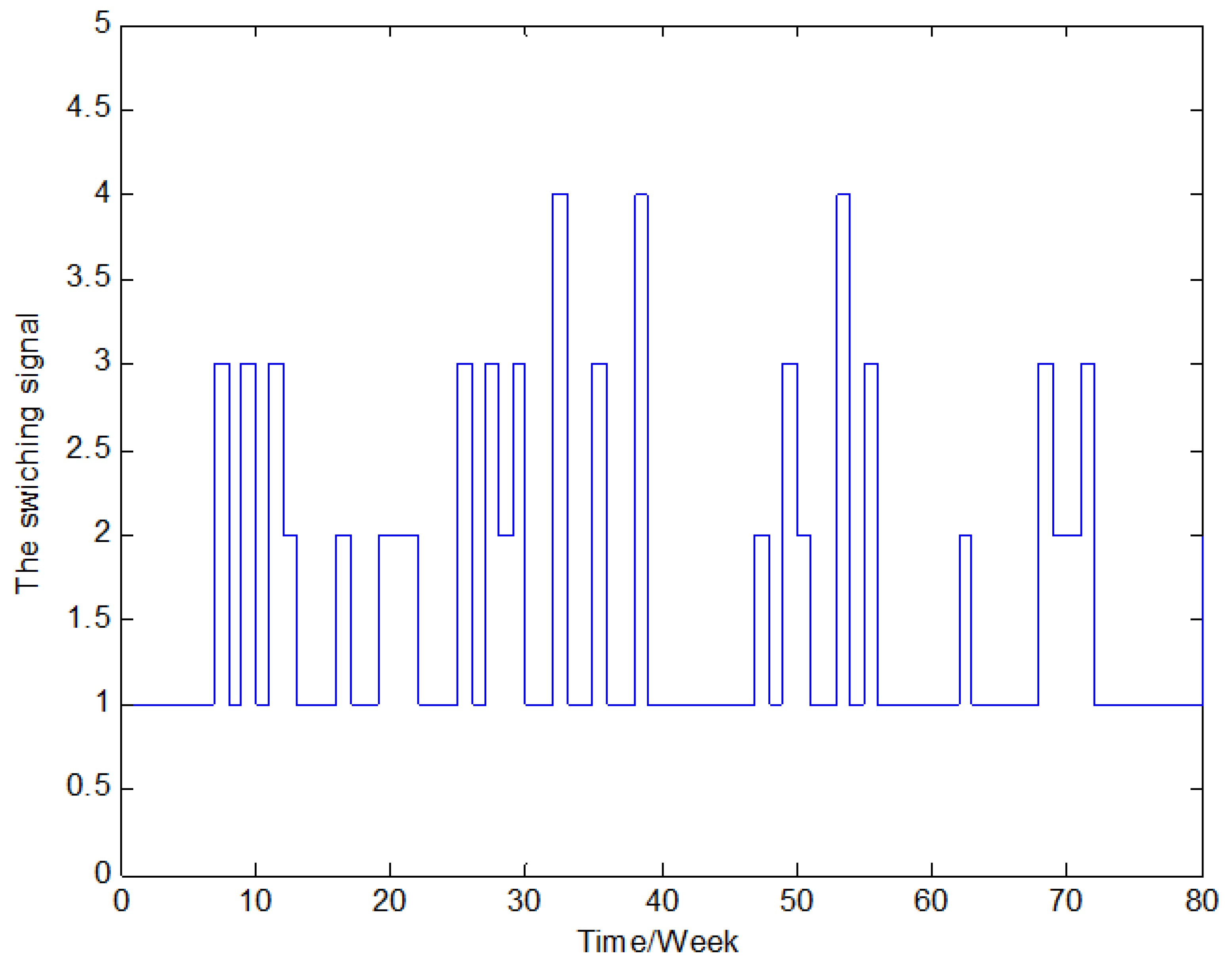
In the following, we consider the robust $H_{\infty }$ control problem for a system with both external demand uncertainty and remanufacturing process uncertainty. Assuming that the external demand uncertainty $\omega \left(k\right)$ is a sinusoidal disturbance, Figure 1 represents the switching signal of a supply chain switching system with Markov jump parameters.

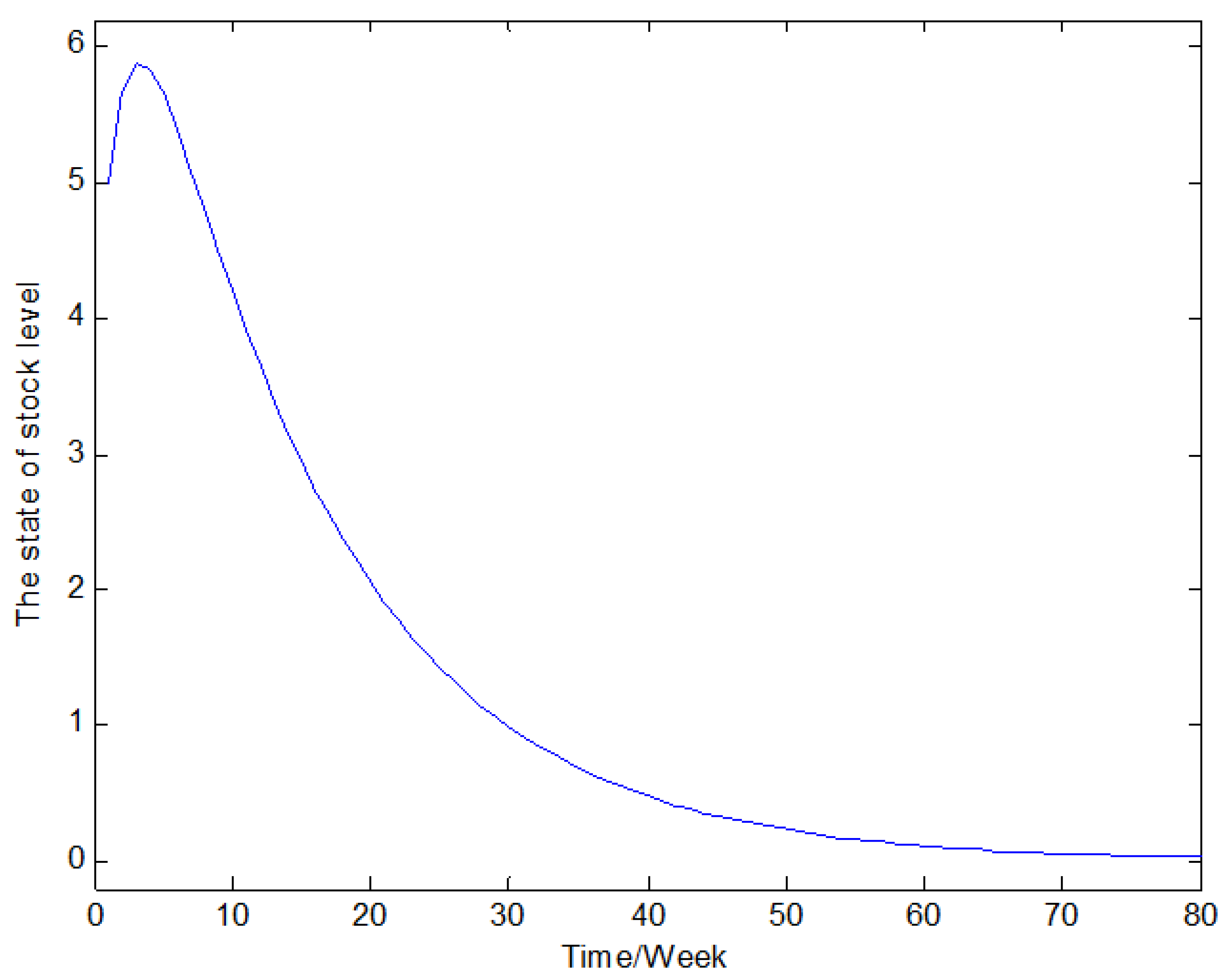
Figure 2 shows the change in stock levels of available commodity warehouses in the presence of external disturbances to the system in the form of sinusoidal disturbances and in the presence of recovery and remanufacturing uncertainty.

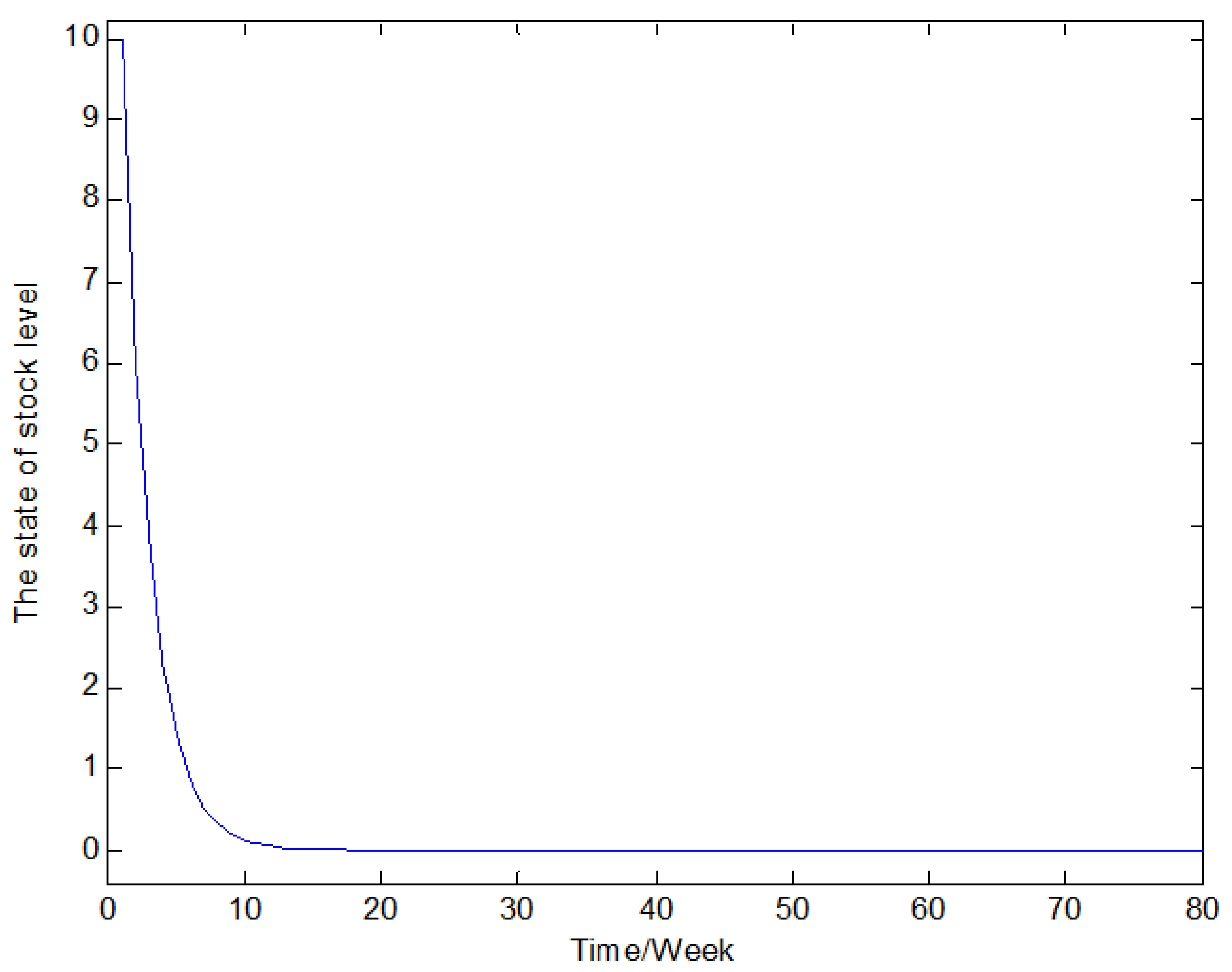
Figure 3 shows the change in stock levels in the recycled goods warehouse in the presence of external disturbances in the form of sinusoidal disturbances in the system and in the presence of uncertainty in recycling and remanufacturing.

From the simulation results, it can be seen that the robust $H_{\infty }$ controller designed in this paper can effectively suppress the uncertain demand disturbance in the recycling and remanufacturing process for the closed-loop supply chain system with Markov jump parameters.

6. Conclusions

In this paper, a closed-loop supply chain system is modeled as a switching system with Markov jump parameters, and the $H_{\infty }$ control problem is studied. The horizontal states of different inventories are determined as four subsystems, and it is assumed that the switching between them has Markov properties. The sufficient conditions to ensure exponential stability of the system and $H_{\infty }$ performance of suppressing the bullwhip effect are given by using LMI form. Simulation examples show the validity of the results obtained.