NAMRTNet: Automatic Classification of Sleep Stages Based on Improved ResNet-TCN Network and Attention Mechanism

Abstract

Sleep, as the basis for regular body functioning, can affect human health. Poor sleep conditions can lead to various physical ailments, such as poor immunity, memory loss, slow cognitive development, and cardiovascular diseases. Along the increasing stress in society comes with a growing surge in conditions associated with sleep disorders. Studies have shown that sleep stages are essential for the body’s memory, immune system, and brain functioning. Therefore, automatic sleep stage classification is of great medical practice importance as a basis for monitoring sleep conditions. Although previous research into the classification of sleep stages has been promising, several challenges remain to be addressed: (1) The EEG signal is a non-smooth signal with harrowing feature extraction and high requirements for model accuracy. (2) Some existing network models suffer from overfitting and gradient descent. (3) Correlation between long time sequences is challenging to capture. This paper proposes NAMRTNet, a deep model architecture based on the original single-channel EEG signal to address these challenges. The model uses a modified ResNet network to extract features from sub-epochs of individual epochs, a lightweight attention mechanism normalization-based attention module (NAM) to suppress insignificant features, and a temporal convolutional network (TCN) network to capture dependencies between features of long time series. The recognition rate of 20-fold cross-validation with the NAMRTNet model for Fpz-cz channel data in the public sleep dataset Sleep-EDF was 86.2%. The experimental results demonstrate the network’s superiority in this paper, surpassing some state-of-the-art techniques in different evaluation metrics. Furthermore, the total time to train the network was 5.1 h, which was much less than the training time of other models.

1. Introduction

Sleep is an inherently complex physiological process in humans, and sleep disorder problems can seriously endanger human health, such as memory loss, mental discomfort, and the induction of cardiovascular diseases [1]. Everyone goes through a periodic cycle of sleep stages during sleep, and those with sleep disorders will develop problems with inconspicuous or confusing processes. In 2020, the COVID-19 pandemic led to a large regional sequestration and an increasing number of people with sleep disorders, especially women [2]. Therefore, accurate classification of sleep stages is critical in diagnosing and treating sleep disorders.

Typically, polysomnography (PSG), also known as a sleep study, is a clinically approved sleep monitoring device that is used to assess sleep quality. The data recorded by PSG includes various physiological signals such as electroencephalography (EEG), electromyography (EMG), electrocardiography (ECG), and other environmental signals [3]. Clinically, sleep specialists classify sleep into five stages according to the sleep staging criteria of the AASM (American Academy of Sleep Medicine): W, N1, N2, and N3, REM. The need for manual classification and statistical analysis of sleep stages based on the characteristics of brain waves during different sleep periods and personal experience makes manual sleep staging a tedious and time-consuming task, and the staging results are highly subjective [4]. With the increasing number of people suffering from sleep disorders and the growing impact of other sleep problems, many researchers have developed automatic sleep detection classification based on machine learning and deep learning [5,6,7,8,9,10,11,12,13,14,15,16,17,18,19,20,21,22,23,24,25,26,27].

Based on traditional machine learning, such as decision trees [5], random forests [6,7], and support vector machines [8,9,10], the construction and selection of features for these methods are critical. Standard features can be broadly classified into time domain, frequency domain, time–frequency, and nonlinear features. Considering that all EEG sleep information is contained in the time domain waveform, the first approach is to extract valuable features directly from the time domain. Lubin used spectral analysis to classify EEG signals into five bands: α, θ, δ, β, and σ, and found that δ and σ waves can distinguish sleep states well [11]. After long-term research, the widely used time-frequency analysis methods include the short time Fourier transform [12], wavelet transform [13], and Hilbert–Yellow transform [14]. The nonlinear features are mainly based on entropy and complexity. Although the traditional machine learning-based sleep detection grading method has achieved some results, the feature data extracted by this method is not comprehensive enough, and the accuracy of sleep scoring is not high enough.

With the gradual advancement of research, neural network-based deep learning techniques have attracted a lot of attention from researchers. Compared with traditional machine learning, deep learning can automatically learn multidimensional abstract features of data from different perspectives by overlaying network layers and powerful neurons. Several studies have designed convolutional neural networks (CNNs) [15,16,17,18,19,20,21]. On study [15] developed a high-precision real-time automatic k-complex wave detection system using multiple CNN networks with migration learning to implement a convolutional neural network (faster R-CNN) detector with faster regions. Another study [16] used end-to-end training with two pairs of convolutional layers for filtering, pooling layers for subsampling, a backpropagation algorithm for iterative optimization training, and a class balancing processor for batch sampling to solve typical data imbalance problems. There are 14 layers of networks, with the 30 s epoch as the input, the first two epochs and the last one as the temporal background, and the original signal as a sample, without the need for domain-specific feature extraction methods [17]. On the other hand, [18] proposed a CNN network architecture based on network depth to improve the classification performance of CNNs, which achieved 81% classification accuracy. Ref. [19] Using 90S EEG signal as an epoch as input, the network architecture of superimposed micro-neural network and compression-excitation (SE) block was proposed, which achieved 85.3% accuracy on the Sleep-EDF data set. Furthermore, [20] used a two-dimensional convolutional network to classify raw data from three channels (i.e., EEG, ECG, and EMG). Finally, [21] proposed a fast convolution method that uses 1D convolution and a layered Softmax method in the classification layer to improve computational efficiency. CNN models have achieved some results in automatic sleep classification, but it is clear that hand-designed features perform better than the original signal. It may be since when sleep experts score the sleep stages of a period, they usually find sleep-related events (e.g., frequency components: α, β, δ, and θ, k-complex, sleep spindle) in that period. The relationship between sleep stages of adjacent periods is then analyzed. The CNN model does not consider the temporal information the sleep expert uses in determining the sleep stages in each period. In addition, the CNN network has certain limitations that lead to a less-than-optimal model, so the application of an improved network is warranted.

Some researchers have started to apply RNNs (recurrent neural networks) to sleep staging [22,23,24,25,26,27]. RNN is able to maintain internal memory, condition historical information, and learn temporal information from input sequences using feedback connections. Their main strength is that they can be trained to understand patterns of variation between EEG signals and to obtain a temporal correlation of the data, for example, to identify the next possible sleep stage in a series of ephemeral information transformation rules [22]. Elman [23] used RNNS to provide both feedforward and feedback connection channels, facilitating the capture of relevant information before and after sleep. Another study [24] used RNNs to obtain information about the time interval at which CNNs acquire features in each epoch, using a sleep staging model based on a single-channel EEG signal, using CNNs with different convolutional ker-nels to extract features from the original signal separately and then feeding them into a long short-term memory (LSTM) for learning, on the publicly available dataset Sleep-EDF obtained an overall accuracy of 82.0%. Phan et al. [25] used RNN to analyze representative features extracted from sub-epochs within the temporal context within and between epochs, achieving an accuracy of 85.3% on the Sleep-EDF dataset. Furthermore, [26] used a combination of CNN and LSTM to extract the time–frequency features and learning time information of EEG signals and train a classifier for sleep staging. Finally, [27] proposed a sleep learning segmentation algorithm based on low sampling frequency pressure sensing signals. Convolutional neural networks were used to extract sleep segmentation features, and LSTM neural networks were used to extract time series features. The results show that considering both intra-epoch and inter-epoch temporal context is beneficial to improve automatic sleep scoring. However, LSTM has many structural parameters, complex computations, and long model training time, which affects the training efficiency of the model [28].

This paper proposes NAMRTNet, an automatic sleep stage staging model based on an improved hybrid network ResNet-TCN and NAM attention mechanism. NAMRTNet analyzes the temporal context mainly at the level of epochs and sub-epochs and uses an enhanced ResNet network combined with the NAM attention mechanism to encode each epoch of EEG signal sub-epochs into corresponding representative features, and suppress the insignificant features and ignore the noise effects. The temporal features are then obtained using TCN networks to learn the transition rules between phases and solve the dependence problem of long-time sequences. NAMRTNet is an end-to-end deep learning-based model that uses the original single-channel Fpz-cz signal without any data pre-processing operation. Extensive experiments on the dataset Sleep-EDF show that the NAMRTNet model outperforms some state-of-the-art techniques for automatic sleep stage classification. The network in this paper achieves an accuracy of 86.2%, and due to the TCN network’s parallelism, the NAMRTNet model’s training time is 5.1 h, which is significantly less than other models, effectively saving resources.

The remainder of the paper is organized as follows: Section 2 presents the basic framework of the model and some improvements to this paper. Section 3 describes the dataset and evaluation metrics, the comparison experiments, the network parameter settings, the sleep stage score performance, and the comparison results against state-of-the-art methods. Finally, in Section 4, the work of this paper is summarized.

2. Materials and Methods

2.1. Dataset

In this paper, we chose the publicly available dataset Sleep-EDF, which includes PSG records labeled by human sleep experts and the corresponding sleep stages. The Sleep-EDF dataset comprises two sets of subjects, one of the healthy subjects SC without sleep-related disorders and the second of subjects ST with temazepam effects on sleep. As the Fpz-cz channel is more suitable than the Pz-oz channel data for sleep stage staging, this paper uses the EEG signal from the Fpz-cz channel at a sampling rate of 100 hz without any pre-processing operations. All recordings within the dataset will be divided into multiple 30 s segments, each segment symbolizing a stage, and the sample distribution of the Sleep-EDF dataset is shown in

Table 1. Number of epochs by class in the dataset.

Dataset	W	N1	N2	N3	REM	Total
Sleep-EDF	8285	2804	17,799	5703	7717	42,308

.

2.2. Model Overview

This section introduces the NAMRTNet network model of this paper. Figure 1 shows the overall architecture of the NAMRTNet network model.

Sleep experts performing sleep stage staging will observe the frequency characteristics of the EEG signal and the transition relationships between these sleep-related events, such as the k-complex and sleep spindle waves. In this paper, we retrieve sub-epoch (as shown in the purple box in Figure 1 features from the 30 s (one epoch) EEG signal with a modified ResNet network to learn sleep-related events, and the attention module suppresses the unimportant features. Then, temporal features are obtained at the ephemeral and sub-ephemeral levels with a TCN network to learn transition rules between sleep stages, and finally, sleep stages are classified [29].

Precisely, to extract more productive features, this paper uses a method of dividing the 30 s EEG sequence into k-segment series (each sequence is a sub-epoch), with representative features of each segment extracted by a modified ResNet and NAM network. In addition, to capture the changes experienced by the transitions between each stage, each segment sequence contains some overlapping features of the previous segment. The orange box in Figure 1 shows the features extracted by the ResNet and attention networks. The extracted ones are then sent in left-to-right order to the TCN network for final classification. The TCN network can learn the dependencies between features of long-time sequences, and in order to analyze the temporal contextual relationships, four epochs are input in this paper, which can study the transition rules between sleep stages at both epoch and sub-epoch levels, capturing the temporal correlation between sequences the temporal correlation. Finally, the activation function softmax completes the classification output for the sleep phase. Next, the paper describes the individual modules in detail.

2.3. Multi-Sub-Epoch Feature Learning

Figure 2 displays the network structure of feature extraction at the sub-epoch level in this paper, consisting of an improved ResNet 34 and attention mechanism (MRNANet). MRNANet extracts the features of each sub-epoch, the NAM attentional mechanism is used to reduce the weight of less significant features, and then establish a feature sequence for each epoch.

$$\left\{f_{1,1},f_{1,2},\dots ,f_{1,h}\right\}$$

(1)

The output feature sequence of 4 epochs can be expressed as:

$$F=\left\{f_1,f_2,f_3,f_4\right\}=\left\{f_{1,1},f_{1,2},\dots ,f_{1,h},\dots ,f_{4,1},\dots ,f_{4,h}\right\}$$

(2)

$f_{i,j}$ is the representative feature of the $j$ sub-epoch and of the $i$ epoch. The last layer, the pooling layer, can filter out useful features from many features to prevent over-fitting problems in classification tasks. MRNANet will be introduced in detail below.

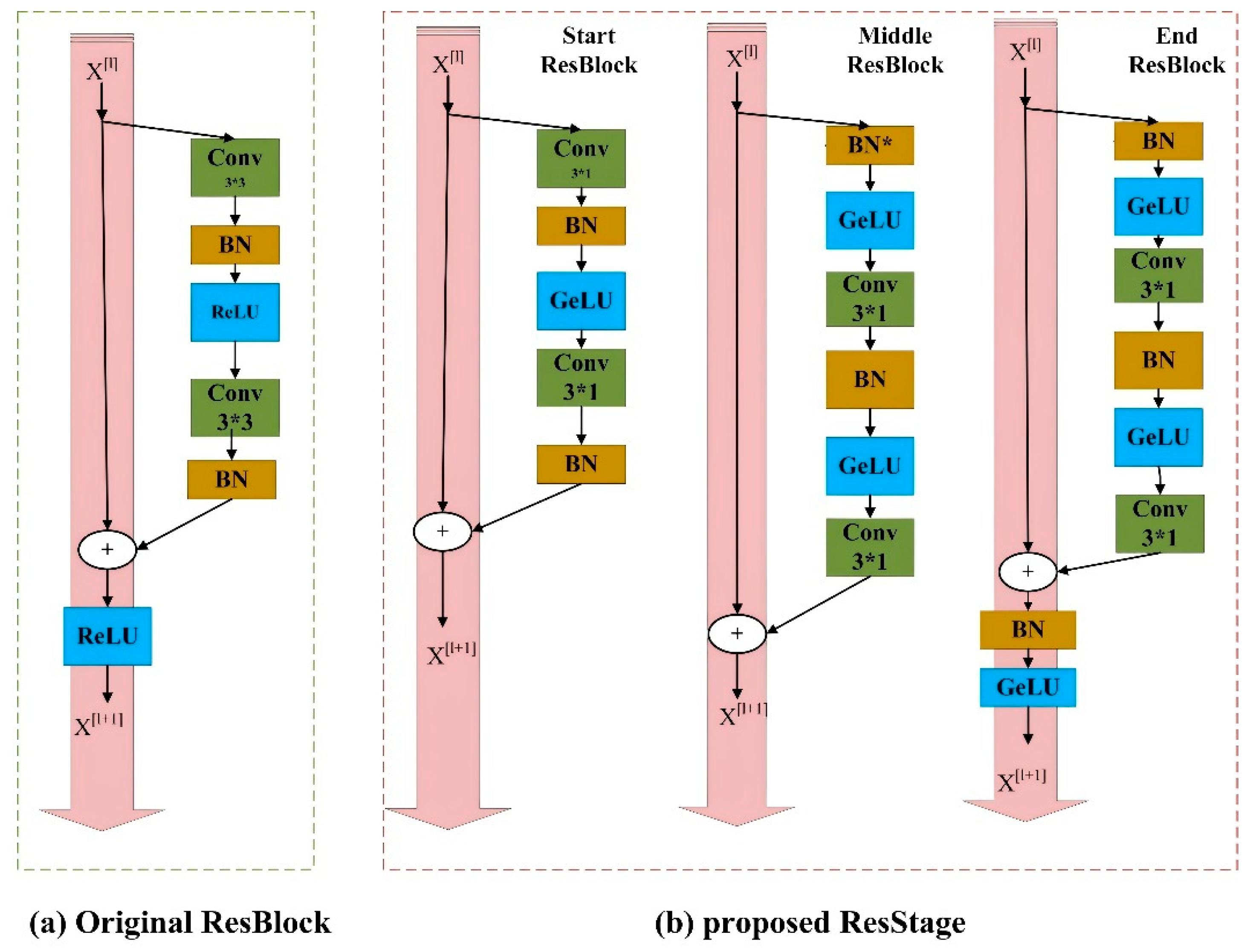
2.4. Improved ResNet 34

ResNet 34 for this article includes a start-up phase, four major phases, and a dropout layer. Each central stage consists of several ResBlocks.

Figure 3a, the original ResBlock bottleneck, contains two convolution layers (one convolution layer kernel is 1 × 1 and another is 3 × 3), two batch normalizations, and two ReLUs. The gray arrow in the original ResBlock represents information transmission, and the $\mathrm{Re}LU$ activation function exists on its path. $\mathrm{Re}LU$ will return to zero when it meets a negative signal, which may cause inaccurate information transmission.

Figure 3. Residual component architecture: (a) original [30]; (b) proposed ResStage. (The first $BN$ in the first intermediate Resblock is eliminated at each stage, * represents multiplication sign).

Figure 3. Residual component architecture: (a) original [30]; (b) proposed ResStage. (The first $BN$ in the first intermediate Resblock is eliminated at each stage, * represents multiplication sign).

Each of the four major phases of the improved ResNet 34 consists of a start ResBlock, an end ResBlock, and an intermediate ResBlock. Figure 3b demonstrates three differences between these three residual blocks. First, we changed the kernel of all convolution layers to 1 × 1, so one-dimensional processing is more suitable for electrical signals. Secondly, the distribution is different. In the start ResBlock, after the last convolution, there is a batch normalization ($BN$) layer ready to add elements using the projection shortcut. The end Resblock ends with the BN layer and Gaussian error linear unit activation function ($GeLU$). The end ResBlock is the preparation for the next phase of execution, which allows information to flow more smoothly across the network. Finally, the $GeLU$ function replaces each residual block’s original linear rectifier function ( $ReLU$ ). The form of the $ReLU$ function is:

$$\mathrm{Re}LU\left(x\right)=\max \left(0,x\right)$$

(3)

which determines that when using the $ReLU$ activation function in calculating the gradient, if many values are lower than 0, there will be many differences. The weights and biases will be updated. The $GeLU$ function has the form:

$$GeLU\left(x\right)=0.5x\left(1+\tanh \left(\sqrt{2/\pi }\left(x+0.044715x^3\right)\right)\right)$$

(4)

It can effectively solve the problem of negative input, so we replace all $ReLU$ functions with $GeLU$ functions.

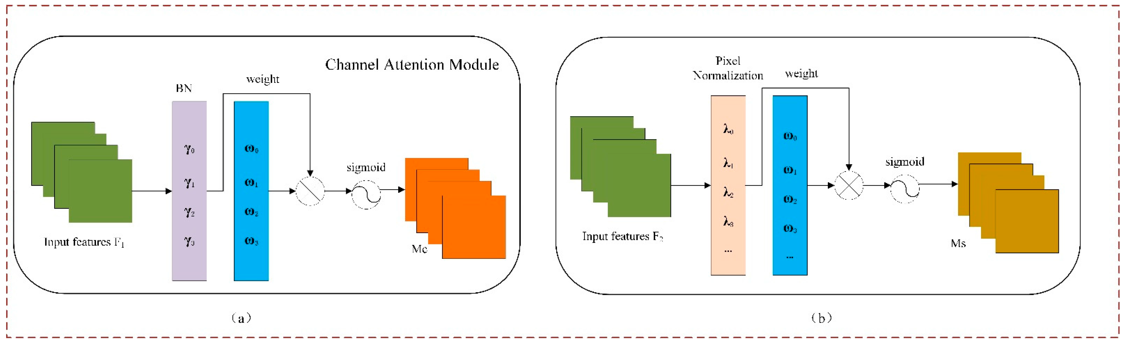
2.5. NAM Attention Mechanism

An improved channel spatial attention mechanism is added to precede the bare block and dropout layers in the improved ResNet 34 network to suppress less significant features in neural network channels or spaces. NAM, a lightweight attention mechanism used in this paper, adopts the module integration approach of CBAM [31]. It applies a sparse weight penalty to attention modules, which can not only maintain similar performance but also make their calculation efficiency higher.

The channel attention module is shown in Figure 4a, and we apply the scale factor in batch normalization ($BN$) to the channel dimension.

$$B_{out}=BN\left(B_{in}\right)=\gamma \frac{B_{in}-{\mu }_B}{\sqrt{{\sigma }_B^2+\epsilon }}+\beta$$

(5)

${\mu }_B$ is the mean of mini-batch $B$, and ${\sigma }_B$ is the standard deviation of mini-batch $B$. $\gamma$, and $\beta$ are trainable affine transformation parameters (scale and displacement), through the scaling factor measures the variance of the channel [32], the more significant the dissent, said the more meaningful the channel change, and the information contained in the channel would be more abundant, and more critical, those channels with little variation in variance, with single information and little importance, can be ignored.

The formula for the output feature is $M_c$:

$$M_c=\mathrm{s}igmoid\left(W_{\gamma }\left(BN\left(F_1\right)\right)\right)$$

(6)

The formula for the weight is:

$$W_{\gamma }=\frac{{\gamma }_i}{{\displaystyle {\sum }_{j=0}{\gamma }_j}}$$

(7)

As shown in Figure 4b, we apply the scaling factor in batch normalization ($BN$) to the spatial dimension, outputting features $M_s$:

$$M_s=sigmoid\left(W_{\lambda }\left(B{N}_S\left(F_2\right)\right)\right)$$

(8)

The formula for the weight is:

$$W_{\gamma }=\frac{{\lambda }_i}{{\displaystyle {\sum }_{j=0}{\lambda }_j}}$$

(9)

In the two submodules, $\lambda$ and $\gamma$, are scaling factors, and the loss function can be expressed as:

$$Loss={\displaystyle {\sum }_{\left(x,y\right)}l\left(f\left(x,W\right),y\right)}+p{\displaystyle \sum g\left(\gamma \right)}+p{\displaystyle \sum g\left(\lambda \right)}$$

(10)

The regularization terms $g\left(\gamma \right)=\left|\gamma \right|$$g\left(\lambda \right)=\left|\lambda \right|$ are added to the loss function. While p is used to balance $g\left(\gamma \right)$ and $g\left(\lambda \right)$, the last two terms are the regularization of the scale factor.

2.6. Long Time Series Dependencies

Due to the limitation of the convolution kernel, the traditional convolutional neural network is unsuitable for modeling timing problems. Recent studies have found that specific convolutional structures can achieve better results [33]. At first, the extended convolution of TCN was used to capture the long time mode. TCN can not only avoid the gradient disappearance and gradient explosion of RNN but also achieve the effect of modeling long time series. The TCN model uses the transformation of a one-dimensional fully convolutional network [34] to predict sequences, passing the sequence information through its multilayer network layer by layer until the prediction result is obtained.

Specifically, the length of each EEG characteristic output by the modified ResNet block is $\mathrm{T}:\left\{f_1,\dots ,f_T\right\}$, through the TCN network, which can produce the predictive output of the same length $\mathrm{Z}:\left\{z_1,\dots ,z_T\right\}$. The structure of the TCN model is shown in Figure 5a. It can satisfy the $f:f^{T+1}\to z^{T+1}$ mapping relationship, and because the causal limit, $z_T$ only depends on the $\left\{f_1,\dots ,f_T\right\}$, i.e., at time $t$, the extended convolution’s output depends only on time t and the inputs of the previous layer, not on any future inputs.

The formula of extended convolution is defined as follows:

$$H(K)={\sum }_{i=0}^{j-1}f(i)·X_{k-d·i}$$

(11)

where $d$ is the expansion factor, $j$ is the filter size, and $k-d\ast i$ represents the past direction. When $d=1$, the dilation convolution becomes a regular convolution, and the input range increases as d increases [35]; Figure 5c shows the change in the TCN network’s field of view for $d=3$. Thus, each layer of the TCN network can increase the perceptual field of the TCN by increasing the dilation factor d or the filter size k [36], where the compelling history of one such layer is $\left(j-1\right)\ast d$.

If we define $L$ as the number of samples required for each iteration and derive a vector $z=\left\{z_i\right\}$, where $i=1,2,\dots$ at each time step, the network $F$ is created by minimizing the predicted value with the proper label. The expected loss is calculated between:

$$F^{*}=F^{\min }loss\left(f_1,\dots ,f_L,z_1,\dots z_T\right)$$

(12)

At layer $i$ of the network:

$$d=O\left(2^i\right)$$

(13)

This ensures that there are some filters to capture each input [32], thus achieving a long and compelling history. The residual block shown in Figure 5b is used to accelerate convergence and stability training. Residual connections can train deep networks and transfer information across layers. Each residual block has two convolution and nonlinear mappings that regularize the network using the WeightNorm and Dropout. A 1 × 1 convolution reduces the dimension and solves the inconsistency of the number of channels in the feature graph. The residual block contains a branch whose output is added to the block’s input $x$ through a series of transformations:

$$O=Activation\left(x+\phi \left(x\right)\right)$$

(14)

This effectively allows layers to learn changes to the identity map rather than the entire transformation, which has repeatedly proven beneficial for deep networks. In addition, the $GeLU$ function is still used as the activation function in TCN residual block.

3. Results and Discussion

3.1. Evaluation Metrics

To fully evaluate the model named NAMRTNet, we used four parameters: accuracy ($ACC$), Cohen Kappa ($\kappa$) [37], F1 score ($F1$), and $MF1$:

$$ACC=\frac{{\displaystyle {\sum }_{i=1}^N{e}_{ii}}}{{\displaystyle {\sum }_{i=1}^N{\displaystyle {\sum }_{j=1}^N{e}_{ij}}}}$$

(15)

$$\kappa =\frac{ACC-p_e}{1-p_e}$$

(16)

$$p_e=\frac{{\displaystyle \sum _{N=1}^N{a}_N\times b_N}}{K\times K}$$

(17)

$$F1=\frac{2}{\frac{1}{\mathrm{P}R}+\frac{1}{RE}}$$

(18)

$$PR=\frac{e_{ii}}{{\displaystyle {\sum }_{j=1}^N}eij}$$

(19)

$$RE=\frac{e_{ii}}{{\displaystyle {\sum }_{j=1}^N}eji}$$

(20)

$$MF1=\frac{{\displaystyle {\sum }_{N=1}^N}F1}{N}$$

(21)

where $e_{ij}$ represents the elements of the ith row and jth column, $N$ is the number of categories, $K$ is the total number of epochs, $PR$ represents the accuracy of distinguishing sleep stages from other stages, $RE$ represents the accuracy of predicting sleep stages, $a_N$ represents the number of epochs of the Nth category, and $b_N$ represents the number of epochs predicted to be the Nth category.

3.2. Parameters of the Optimizer

Under the condition of no data pre-processing, the Ndam optimizer is used. To avoid overfitting, L2-Norm regularization methods include weight_decay = ${10}^{-6}$, a batch training size of 64, and learning_rate = 0.001. This study did not use any balanced data processing or model training methods. We followed the training for ten consecutive sessions using a cost-tracking approach and stopped training when no improvement was shown. For each fold cross-validation, the best model in the test set was selected for evaluation. This study did not use any method of balancing data processing or model training to achieve an early stop by tracking the validation cost. The training process is implemented in python 3.6.13 and pytorch 1.10.1, on the RTX 3070.

3.3. ResNet Layer Number Settings

In order to improve the model performance, this study aimed to select the optimal number of network layers for ResNet. Figure 6 shows the results of experiments with 20-fold cross-validation on the sleep-EDF dataset with different network layers (18, 34, 50, 101, and 152). When the number of network layers is 34, the accuracy, F1 score, and Cohen’s Kappa (κ) are significantly higher than the other network models. Therefore, the number of layers of ResNet is chosen to be 34 in this paper to ensure the depth features that can be extracted effectively without degrading the network performance.

3.4. TCN Hidden Layer Setting

It is vital to select the number of channels of TCN hidden layers. Too few channels will lead to a decrease in the learning ability of the network and even a decrease in the ability to predict information. Conversely, too many choices will lead to a more complex network. Such a network not only fails to improve its performance but also tends to fall into local minima during the training process, which will reduce the learning speed of the network. In order to select the most suitable number of hidden layers, the network performance is tested in this paper when the hidden layers are 32 × 1, 64 × 1, 128 × 1, and 64 × 1. Figure 7 shows the comparison results of recognition rate, F1 score, and Cohen’s Kappa (κ) with different numbers of channels. It is clear that the 64 × 1 network model has better learning ability.

3.5. Comparative Experiments

The NAMRTNet in this paper consists of the modified ResNet-34, the NAM attention mechanism, and the TCN network. Two comparative studies were carried out to analyze the effectiveness of the network modules of NAMRTNet in this paper. The first group was ResNet+TCN (ResNet 50) and ResNet+TCN (modified ResNet 50). As ResNet-TCN does not support a 34-layer network structure, the exact condition of network level 50 was chosen for validation in order to verify the effectiveness of the modules in this paper.

As shown in Figure 8, the accuracy, F1 score, and Cohen’s Kappa (κ) of the improved ResNet network were 84.8, 77.7, and 0.79, respectively, which were higher than the results of the original network (85.8, 79.0, and 0.804). According to the confusion matrix results, N1, N3, and REM are the main stages with a facilitative effect. Thus, the improved network can effectively improve the problem of inaccurate information transfer, and the one-dimensional convolution is more suitable for such long time series of EEG data. Placing Max-pool between the Conv3x and Conv4x layers also reduces the length of the feature sequence by half, reducing the parameters and enhancing the expressiveness of the network.

The second set of experiments was designed to verify the effectiveness of TCN. The comparison results of ResNet+NAM+LSTM (improved ResNet 34) and ResNet+NAM+TCN (improved ResNet 34) are shown in Figure 9. The application of TCN network structure improves the final recognition rate by 2.2%, and the prediction of each stage is enhanced to a certain extent, indicating that TCN can capture the time correlation of long time series well, and the improved network structure can overcome the imbalance of PSG data to a certain extent.

3.6. K-Fold Crossover Experiment

To better represent the network performance, cross-validation experiments (10-fold, 15-fold, and 20-fold) were performed in this paper to find the best classification for the dataset and to avoid the selection of unexpected hyperparameters and models that cannot generalize due to particular classifications. The results in

Table 2. The 10, 15, and 20-fold cross-validation results.

K-Folds	Overall Performance			Per-Class Performance
	Acc	MF1	κ	W	N1	N2	N3	REM
10	83.7	76.4	0.77	90.7	35.8	88.9	90.4	86.8
15	84.8	77.9	0.793	90.3	39.9	88.9	86.3	83.9
20	86.2	79.8	0.808	92.0	45.5	89.4	88.6	83.5

show that the evaluation metrics, such as classification accuracy (PR), classification F1 score (F1), and overall accuracy (Acc) of the experiments, conducted with 20-fold cross-validation are better than the other methods, so the dataset partitioning method of randomly dividing the subjects into training, validation, and test sets in the ratio of 15:4:1 maximizes the model performance.

3.7. Sleep Stage Scores

As shown in

Table 3. Confusion matrix obtained from 20-pass cross-validation on the Fpz-cz channel of the sleep-EDF dataset.

Method	Predicted					Per-Class Metrics
	W	N1	N2	N3	REM	PR	RE	F1
W	7497	393	153	24	123	92.6	91.5	92.0
N1	442	1122	683	15	640	55.2	38.7	45.5
N2	77	223	16,416	625	804	88.4	90.5	89.4
N3	8	0	609	5009	0	88.1	89.0	88.6
REM	76	295	711	12	6749	81.2	86.1	83.5

, the confusion matrix is calculated by summing the scored values of all test data. Each row represents the number of samples classified by the expert, and each column represents the number of epochs predicted by the model. The table also shows the accuracy, recall, and F1 score for each category. According to the confusion matrix, the values in the diagonal position are higher than the other values, which proves that the NAMRTNet model is adequate. In addition, the score of F1 can reach 92.0 in stage W, 89.4 in stage N2, and 88.6 in stage N3. Due to the similarity of the signal characteristics of the N2 and REM periods, it may need to be more accurate in the classification process. The REM stage F1 score is 83.5, and these four stages are above 80. We need to care that the N1 stage score is relatively low. First of all, from Table 1, it can be seen that the number of N1 stage samples is only 2804, which is far less than other stages. In addition, for N1, as a transition period, there will be many confusing features before and after the transition period, which causes great difficulties for staging.

3.8. Comparison with the Forward Approach

Table 4. Comparison of NAMRTNet with other methods.

Method	Overall Performance			Per-Class Performance
	Acc	MF1	κ	W	N1	N2	N3	REM
1-max CNN [38]	79.8	72.0	0.720	-	-	-	-	-
VGG-FT [39]	80.3	-	-	-	-	-	-	-
SleepEEGNet [40]	84.26	79.66	0.79	89.19	52.19	86.77	85.13	85.02
CCRRSleepNet [41]	84.29	79.81	0.78	89.01	51.73	87.25	88.20	82.86
AttnSleep [42]	84.3	77.7	0.776	85.4	50.9	88.8	86.4	86.5
FT DeepSleepNet+ [43]	84.4	78.8	0.781	-	-	-	-	-
IITNet [44]	84.6	79.0	0.782	81.0	50.5	88.2	86.9	87.2
FT SeqSleepNet+ [43]	85.2	79.6	0.789	-	-	-	-	-
TinySleepNet [45]	85.4	80.5	0.80	90.1	51.4	88.5	88.3	84.3
proposed Method	86.2	79.8	0.808	92.0	45.5	89.4	88.6	83.5

compares our approach with existing methods. The improved 1-max CNN of [38] is used in combination with a DNN learning frequency domain filter bank to pre-process time–frequency image features. VGG-FE [39] utilizes multi-cone spectroscopy, a typical migration learning approach. SleepEEGNet [40] proposes a CNN-BIRNN network architecture along with a loss function to tackle the issue of class imbalance within EEG datasets. CCRRSleepNet [41] uses hybrid relational induced bias to optimize the network and uses multiple convolutional blocks to extract complex features. AttnSleep [42] utilizes small-core and wide-core dual-branch CNN to extract features of different frequencies and use a multi-head attention (MHA) mechanism to capture time dependencies between features. Furthermore, [43] used migration learning with SeqSleepNet+ and DeepSleepNet+ based on a sequence-to-sequence sleep staging framework to overcome the problem of small datasets and insufficient data in sleep studies. IITNet [44] utilizes ResNet and LSTM to learn the time context within and between epochs of learning. TinySleepNet [45] simplifies the DeepSleepNet model structure and incorporates data augmentation. Overall, our method is relatively novel and achieves better performance because the shared convolutional structure allows the TCN to process long sequences in parallel, so the TCN is more memory efficient than the recurrent network, thus, the training time is shorter, with a total cross-validation time of 5.1 h for 20 folds, which is significantly better than [42] (about 7 h).

4. Conclusions

This paper proposes a new network structure, NAMRTNet, to classify raw single-channel EEG data into sleep stages. NAMRTNet consists of two parts. First, a modified ResNet-34 network combined with the NAM attention mechanism extracts ephemeral invariant features to improve the network effectively. Then, the TCN network is used to learn the dependencies between long time sequences. Experimental results on the Sleep-EDF dataset show that the model proposed in this paper is superior to some state-of-the-art methods for a variety of evaluation metrics.

Furthermore, from the experimental procedure, the training time of the model in this paper is significantly outperformed by the literature [42], which is a good indication of the correctness of the choice of the TCN network, which can handle time series efficiently. This paper effectively selects the optimal network experimentally to maximize the model’s performance. Finally, NAMRTNet is end-to-end and does not require pre-processing of the data so that it can be directly used for applications in healthcare and other fields. In the future, we intend to enhance our NAMRTNet so that it can be applied to multimodal signals collected by wearable devices containing EEG, EOG, EMG, etc., to fuse multimodal signals, remove noise interference using state-of-the-art techniques, optimize feature extraction, reduce the impact caused by too little data in the N1 stage, and effectively improve the automatic scoring of sleep stages to improve people’s quality of life effectively.

References

1. Luyster, F.S.; Strollo, P.J., Jr.; Zee, P.C.; Walsh, J.K. Boards of Directors of the American Academy of Sleep Medicine and the Sleep Research Society. Sleep A Health Imp. Sleep 2012, 35, 727–734. [Google Scholar] [CrossRef]
2. Ruiz-Herrera, N.; Díaz-Román, A.; Guillén-Riquelme, A.; Quevedo-Blasco, R. Sleep Patterns during the COVID-19 Lockdown in Spain. Int. J. Environ. Res. Public Health 2023, 20, 4841. [Google Scholar] [CrossRef] [PubMed]
3. Keenan, S.A. An overview of polysomnography. Handb. Clin. Neurophysiol. 2005, 6, 33–50. [Google Scholar]
4. Stepnowsky, C.; Levendowski, D.; Popovic, D.; Ayappa, I.; Rapoport, D.M. Scoring accuracy of automated sleep staging from a bipolar electroocular recording compared to manual scoring by multiple raters. Sleep Med. 2013, 14, 1199–1207. [Google Scholar] [CrossRef] [PubMed] [Green Version]
5. Hassan, A.R.; Bhuiyan, M.I.H. Computer-aided sleep staging using complete ensemble empirical mode decomposition with adaptive noise and bootstrap aggregating. Biomed. Signal Process. Control. 2016, 24, 1–10. [Google Scholar] [CrossRef]
6. Sharma, R.; Pachori, R.B.; Upadhyay, A. Automatic sleep stages classification based on iterative filtering of electroencephalogram signals. Neural Comput. Appl. 2017, 28, 2959–2978. [Google Scholar] [CrossRef]
7. Hassan, A.R.; Bhuiyan, M.I.H. A decision support system for automatic sleep staging from EEG signals using tunable Q-factor wavelet transform and spectral features. J. Neurosci. Methods 2016, 271, 107–118. [Google Scholar] [CrossRef]
8. Koley, B.; Dey, D. An ensemble system for automatic sleep stage classification using single channel EEG signal. Comput. Biol. Med. 2012, 42, 1186–1195. [Google Scholar] [CrossRef]
9. Lajnef, T.; Chaibi, S.; Ruby, P.; Aguera, P.-E.; Eichenlaub, J.-B.; Samet, M.; Kachouri, A.; Jerbi, K. Learning machines and sleeping brains: Automatic sleep stage classification using decision-tree multi-class support vector machines. J. Neurosci. Methods 2015, 250, 94–105. [Google Scholar] [CrossRef]
10. Zhu, G.; Li, Y.; Wen, P. Analysis and classification of sleep stages based on difference visibility graphs from a single-channel EEG signal. IEEE J. Biomed. Health Inform. 2014, 18, 1813–1821. [Google Scholar] [CrossRef]
11. Lubin, A.; Johnson, L.C.; Austin, M.T. Discrimination among states of consciousness using EEG spectra. Psychophysiology 1969, 10, 593–601. [Google Scholar]
12. Griffin, D.; Lim, J. Signal estimation from modified short-time Fourier transform. IEEE Trans. Acoust. Speech Signal Process. 1984, 32, 236–243. [Google Scholar] [CrossRef]
13. Hazarika, N.; Chen, J.Z.; Tsoi, A.C.; Sergejew, A. Classification of EEG signals using the wavelet transform. Signal Process. 1997, 59, 61–72. [Google Scholar] [CrossRef]
14. Huang, N.E. Hilbert-Huang Transform and Its Applications; World Scientific: Singapore, 2014. [Google Scholar]
15. Khasawneh, N.; Fraiwan, M.; Fraiwan, L. Detection of K-complexes in EEG waveform images using faster R-CNN and deep transfer learning. BMC Med. Inform. Decis. Mak. 2022, 22, 297. [Google Scholar] [CrossRef]
16. Tsinalis, O.; Matthews, P.M.; Guo, Y.; Zafeiriou, S. Automatic sleep stage scoring with single-channel EEG using convolutional neural networks. arXiv 2016, arXiv:1610.01683. [Google Scholar]
17. Sors, A.; Bonnet, S.; Mirek, S.; Vercueil, L.; Payen, J.-F. A convolutional neural network for sleep stage scoring from raw single-channel EEG. Biomed. Signal Process. Control. 2018, 42, 107–114. [Google Scholar] [CrossRef]
18. Sokolovsky, M.; Guerrero, F.; Paisarnsrisomsuk, S.; Ruiz, C.; Alvarez, S.A. Deep learning for automated feature discovery and classification of sleep stages. IEEE/ACM Trans. Comput. Biol. Bioinform. 2019, 17, 1835–1845. [Google Scholar] [CrossRef] [Green Version]
19. Li, F.; Yan, R.; Mahini, R.; Wei, L.; Wang, Z.; Mathiak, K.; Liu, R.; Cong, F. End-to-end sleep staging using convolutional neural network in raw single-channel EEG. Biomed. Signal Process. Control. 2020, 63, 102203. [Google Scholar] [CrossRef]
20. Chambon, S.; Galtier, M.N.; Arnal, P.J.; Wainrib, G.; Gramfort, A. A deep learning architecture for temporal sleep stage classification using multivariate and multimodal time series. IEEE Trans. Neural Syst. Rehabil. Eng. 2018, 26, 758–769. [Google Scholar] [CrossRef] [Green Version]
21. Yulita, I.N.; Fanany, M.I.; Arymurthy, A.M. Fast Convolutional Method for Automatic Sleep Stage Classification. Health Inform. Res. 2018, 24, 170–178. [Google Scholar] [CrossRef]
22. Berry, R.B.; Brooks, R.; Gamaldo, C.E.; Harding, S.M.; Marcus, C.; Vaughn, B.V. The AASM Manual for the Scoring of Sleep and Associated Events: Rules, Terminology and Technical Specifications; American Academy of Sleep Medicine: Darien, IL, USA, 2015; pp. 1–7. [Google Scholar]
23. Hsu, Y.-L.; Yang, Y.-T.; Wang, J.-S.; Hsu, C.-Y. Automatic sleep stage recurrent neural classifier using energy features of EEG signals. Neurocomputing 2013, 104, 105–114. [Google Scholar] [CrossRef]
24. Supratak, A.; Dong, H.; Wu, C.; Guo, Y. DeepSleepNet: A model for automatic sleep stage scoring based on raw single-channel EEG. IEEE Trans. Neural Syst. Rehabil. Eng. 2017, 25, 1998–2008. [Google Scholar] [CrossRef] [PubMed] [Green Version]
25. Phan, H.; Andreotti, F.; Cooray, N.; Chén, O.Y.; De Vos, M. SeqSleepNet: End-to-End Hierarchical Recurrent Neural Network for Sequence-to-Sequence Automatic Sleep Staging. Neural Syst. Rehabil. Eng. IEEE Trans. 2019, 27, 400–410. [Google Scholar] [CrossRef] [PubMed] [Green Version]
26. Liu, Y.; Fan, R.; Liu, Y. Deep identity confusion for automatic sleep staging based on single-channel EEG. In Proceedings of the 2018 14th International Conference on Mobile Ad-Hoc and Sensor Networks (MSN), Shenyang, China, 6–8 December 2018; pp. 134–139. [Google Scholar]
27. Huang, Y.; Liang, L.W. Joint sleep staging model based on pressure-sensitive sleep signal. IOP Conf. Ser. Mater. Sci. Eng. 2020, 740, 012159. [Google Scholar] [CrossRef]
28. Gers, F.A.; Schmidhuber, J.; Cummins, F. Learning to forget: Continual prediction with LSTM. Neural Comput. 2000, 12, 2451–2471. [Google Scholar] [CrossRef] [PubMed]
29. Zhu, T.; Luo, W.; Yu, F. Convolution- and Attention-Based Neural Network for Automated Sleep Stage Classification. Int. J. Environ. Res. Public Health 2020, 17, 4152. [Google Scholar] [CrossRef] [PubMed]
30. He, K.; Zhang, X.; Ren, S.; Sun, J. Deep residual learning for image recognition. In Proceedings of the IEEE Computer Society Conference on Computer Vision and Pattern Recognition (CVPR), Las Vegas, NV, USA, 27–30 June 2016; pp. 770–778. [Google Scholar] [CrossRef] [Green Version]
31. Woo, S.; Park, J.; Lee, J.Y.; Kweon, I.S. CBAM: Convolutional block attention module. In Proceedings of the European Conference on Computer Vision, Munich, Germany, 8–14 September 2018. [Google Scholar] [CrossRef] [Green Version]
32. Ioffe, S.; Szegedy, C. Batch normalization: Accelerating deep network training by reducing internal covariate shift. In Proceedings of the International Conference on Machine Learning, Lille, France, 6–11 July 2015; pp. 448–456. [Google Scholar]
33. Bai, S.; Kolter, J.Z.; Koltun, V. An empirical evaluation of generic convolutional and recurrent networks for sequence modeling. arXiv 2018, arXiv:1803.01271. [Google Scholar]
34. Long, J.; Shelhamer, E.; Darrell, T. Fully convolutional networks for semantic segmentation. In Proceedings of the IEEE Conference on Computer Vision and Pattern Recognition, Boston, MA, USA, 7–12 June 2015; pp. 3431–3440. [Google Scholar]
35. Lea, C.; Flynn, M.D.; Vidal, R.; Reiter, A.; Hager, G.D. Temporal convolutional networks for action segmentation and detection. In Proceedings of the IEEE Conference on Computer Vision and Pattern Recognition, Honolulu, HI, USA, 21–26 July 2017; pp. 156–165. [Google Scholar]
36. Troncoso, A.; Salcedo-Sanz, S.; Casanova-Mateo, C.; Riquelme, J.C.; Prieto, L. Local models-based regression trees for very short-term wind speed prediction. Renew. Energy 2015, 81, 589–598. [Google Scholar] [CrossRef]
37. Cohen, J. A coefficient of agreement for nominal scales. Educ. Psychol. Meas. 1960, 20, 37–46. [Google Scholar] [CrossRef]
38. Phan, H.; Andreotti, F.; Cooray, N.; Chén, O.Y.; De Vos, M. DNN filter bank improves 1-max pooling CNN for single-channel EEG automatic sleep stage classification. In Proceedings of the 40th Annual International Conference of the IEEE Engineering in Medicine and Biology Society (EMBC), Honolulu, HI, USA, 18–21 July 2018; pp. 453–456. [Google Scholar]
39. Vilamala, A.; Madsen, K.H.; Hansen, L.K. Deep convolutional neural networks for interpretable analysis of EEG sleep stage scoring. In Proceedings of the IEEE 27th International Workshop on Machine Learning for Signal Processing (MLSP), Tokyo, Japan, 25–28 September 2017; pp. 1–6. [Google Scholar]
40. Mousavi, S.; Afghah, F.; Acharya, U.R. SleepEEGNet: Automated sleep stage scoring with sequence to sequence deep learning approach. PLoS ONE 2019, 14, e0216456. [Google Scholar] [CrossRef] [PubMed] [Green Version]
41. Neng, W.; Lu, J.; Xu, L. Ccrrsleepnet: A hybrid relational inductive biases network for automatic sleep stage classification on raw single-channel eeg. Brain Sci. 2021, 11, 456. [Google Scholar] [CrossRef] [PubMed]
42. Eldele, E.; Chen, Z.; Liu, C.; Wu, M.; Kwoh, C.K.; Li, X.; Guan, C. An attention-based deep learning approach for sleep stage classification with single-channel EEG. IEEE Trans. Neural Syst. Rehabil. Eng. 2021, 29, 809–818. [Google Scholar] [CrossRef] [PubMed]
43. Phan, H.; Chén, O.Y.; Koch, P.; Lu, Z.; McLoughlin, I.; Mertins, A.; De Vos, M. Towards more accurate automatic sleep staging via deep transfer learning. IEEE Trans. Biomed. Eng. 2020, 68, 1787–1798. [Google Scholar] [CrossRef] [PubMed]
44. Seo, H.; Back, S.; Lee, S.; Park, D.; Kim, T.; Lee, K. Intra-and inter-epoch temporal context network (IITNet) using sub-epoch features for automatic sleep scoring on raw single-channel EEG. Biomed. Signal Process. Control. 2020, 61, 102037. [Google Scholar] [CrossRef]
45. Supratak, A.; Guo, Y. TinySleepNet: An efficient deep learning model for sleep stage scoring based on raw single-channel EEG. In Proceedings of the 42nd Annual International Conference of the IEEE Engineering in Medicine Biology Society (EMBC), Montreal, QC, Canada, 20–24 July 2020; pp. 641–644. [Google Scholar]
Figure 1. The network structure of NAMRTNet. The green box plots indicate representative features extracted from each sub-epoch (purple boxes), aggregating into a sequence of features for a single epoch (green boxes). We used a sequence of four epochs to explore temporal dependence (orange boxes), (* represents multiplication sign).
Applsci 13 06788 g001
Figure 2. Shows our feature extraction module from the sub-epoch, consisting of an improved ResNet network and attention mechanism (* represents multiplication sign).
Applsci 13 06788 g002
Figure 4. NAM notes the mechanism module, (a) Channel Attention Module; (b) Pixel Normalization.
Applsci 13 06788 g004
Figure 5. (a) TCN network. (b) Residual block of the TCN network. (c) Residual block (k,d), (* represents multiplication sign).
Applsci 13 06788 g005
Figure 6. Comparison results of recognition rate, F1 score, and Cohen’s Kappa (κ) under different network layers.
Applsci 13 06788 g006
Figure 7. Comparison results of recognition rate, F1 score, and Cohen’s Kappa (κ) under different numbers of channels in TCN hidden layer.
Applsci 13 06788 g007
Figure 8. Confusion matrix of ResNet-TCN and improved ResNet-TCN. (a) ResNet 50-TCN confusion. (b) MResNet 50-TCN confusion.
Applsci 13 06788 g008
Figure 9. (a) ResNet + NAM + LSTM (improved ResNet 34) confusion. (b) ResNet + NAM + TCN (improved ResNet 34) confusion.
Applsci 13 06788 g009