Multiple Fano Resonances in Dynamic Resonant Tunneling Processes

Abstract

The existence of Fano resonances in dynamic resonant tunneling (RT) systems has been investigated. Fano resonances are characterized by the appearance of a 100% reflection coefficient in proximity to a high transmission coefficient. For a Fano resonance to appear, a bound state must exist. On the other hand, a resonant tunneling process is characterized by a high transmission and the existence of a quasi-bound state (QBS) instead of a bound one. It has been shown that, by narrowing the width of the barrier, the resonance energy of the QBS gradually decreases and eventually turns into a bound state. Consequently, in a dynamic RT process, there are two scenarios: either a bound state exists, in which case, Fano resonances exist for any barrier width, or a QBS exists, and the barrier should be narrow enough for the Fano resonance to appear. In both cases, the incoming particle’s frequency must be lower than the oscillating well’s frequency. In this work, these resonances are investigated in detail, and both exactly numerically and approximated analytical expressions are derived for both the weak and strong oscillating amplitude regimes. One of the conclusions is that, when the oscillating frequency is low enough, multiple Fano resonances can appear by varying the barrier’s width. Since these resonances are very sharp and zero transmission can easily be detected, this property can be used as a very accurate method for measuring the barrier’s width, even when the particle’s de-Broglie wavelength is much larger than the barrier’s width.

1. Introduction

Tunneling and Resonant Tunneling are quantum processes that are extremely sensitive to a particle’s energy. Consequently, when a system incorporates dynamic structures, its behavior can become much more complex. In general, perturbations, which are introduced into the system, usually tend to increase the tunneling current. This behavior manifests in activation [1,2,3,4,5,6,7,8,9] and the elevator effect [8,9]. However, in some cases, for some specific energies, the tunneling current can be substantially suppressed [10,11,12,13,14,15,16,17,18,19,20]. In particular, it has been shown that 100% reflection occurs in certain cases. This conduct is related to Fano resonances [21,22,23,24,25,26,27,28].

Recently, a different presentation of current suppression and activation was demonstrated. It was shown that, when a particle penetrates an opaque barrier via a varying well, the process can be regarded as if the particle is trapped in a Quasi-Bound Super State (QBSS) [14], in a similar fashion to a Resonant Tunneling process, in which the particle is trapped in a Quasi-Bound State [29,30,31,32]. The difference between these two scenarios is that the QBSS consists of multiple sub-quasi-states. Consequently, when an incoming particle’s energy matches a high-amplitude spectral component of the QBSS, a high transmission occurs, and similarly, when no match occurs, the current is suppressed. It was noted that, at these energies, a destructive interference occurs in the well, which prevents particles from dwelling in this well, therefore preventing a high transmission. In these cases, the current decreases drastically; however, it is not necessarily reduced to zero, i.e., it does not necessarily show Fano behavior. In fact, the same system may exhibit both behaviors for different energies in different cases.

A Fano resonance occurs due to interference between a bound state and a continuum state. It is, therefore, not straightforwardly clear how a Fano resonance appears in a system that exhibits RT behavior. After all, an RT requires a quasi-bound state and not a bound one.

The width of the barrier affects the resonance energy; however, in most research, this phenomenon has received little attention, mainly due to two reasons: first, in a resonant tunneling process, the barrier is usually opaque, and therefore its specific width has a negligible effect on the resonance energy (which predominantly depends on the shape of the potential well), and second, by narrowing the barrier, the resonance’s spectral width increases (i.e., the particle’s dwelling time in the well decreases); therefore, the resonance nature of the process fades away. Therefore, when the barrier is too narrow, it is fruitless to analyze the process as an RT one. This is indeed true in the stationary case, but in the dynamic case, the situation is much more complicated. Some of these effects have been observed in recent research [21,27].

We will show, in the following sections, that, by narrowing the barrier, not only does the resonance energy decrease drastically, but it can also be negative. Therefore, the barrier’s width shrinkage can turn a resonance state into a bound one. Clearly, in a stationary scattering case, the bound state cannot be reached; however, in a dynamic case, the quasi-bound state generates a Fano resonance, which causes 100% reflection. Moreover, since the particle can lose/gain any number of energy quanta, then, if the oscillating frequency is low enough, by changing the barrier’s width, multiple Fano resonances can occur for the same incoming particle’s energy.

2. The Transition from a Resonant State to a Bound State and Its Dependence on the Barrier’s Width

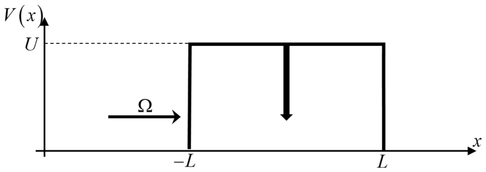
In a stationary Resonant Tunneling process, particles tunnel through an opaque barrier via a quasi-bound state (QBS). A QBS can be formed by locating a potential well within a barrier, as described by the following stationary Schrödinger equation:

$$\left[-\frac{{\partial }^2}{\partial x^2}+U\left(x\right)-\Omega +\mathsf{\alpha }\mathsf{\delta }\left(x\right)\right]\mathsf{\psi }\left(x\right)=0$$

(1)

where $U\left(x\right)=\{\begin{array}{c}U\\ 0\end{array}\hspace{1em}\begin{array}{c}-L<x<L\\ else\end{array}$ is the potential barrier and the potential well is described by a delta function potential. Hereinafter, we use, for simplicity, but without a loss of generality, the units $\hslash =1$ and $2m=1$ for the Planck constant and the electron’s mass, respectively.

The system schematic is presented in Figure 1.

It should be noted that a delta function potential is an excellent approximation for a narrow well, as long as the width of the well is narrower than the De-Broglie wavelength of the QBS [32].

The solution of Equation (1) is:

$$\mathsf{\psi }\left(x\right)={\mathsf{\psi }}_h\left(x\right)+\frac{\mathsf{\alpha }{\mathsf{\psi }}_h\left(0\right)}{1-\mathsf{\alpha }{G}_{\Omega }^{+}\left(0\right)}{G}_{\Omega }^{+}\left(x>L\right)$$

(2)

where ${\mathsf{\psi }}_h\left(x\right)$ is the homogeneous solution (without the well) and $G_{\Omega }^{+}\left(x\right)$ is the outgoing Green function of Equation (1) without the well. For a rectangular barrier, the Green function at $x=0$ is [11,33]:

$$G_{\Omega }^{+}\left(0\right)=-\frac{1}{2\mathsf{\rho }}\coth \left(\mathsf{\rho }L-i\arctan \left(\frac{k}{\mathsf{\rho }}\right)\right)$$

(3)

where $k\equiv \sqrt{\Omega }$ and $\mathsf{\rho }\equiv \sqrt{U-\Omega }$.

In the case of an extremely opaque barrier, i.e., $L\sqrt{U}\gg 1$, the Green function at $x=0$ is approximately $G_{\Omega }^{+}\left(0\right)\cong -1/2\mathsf{\rho }$ and the Resonance Energy of the Opaque Barrier (REOB) is simply:

$${\Omega }_R\left(L\to \infty \right)\equiv U-\frac{{\mathsf{\alpha }}^2}{4}$$

(4)

When the incoming particle’s energy is equal to this resonance energy, the particle will tunnel through the barrier via the QBS with a high probability. Equation (4) is derived for a completely opaque barrier. In general, the resonance energy is a function of the barrier’s parameters (potential height $U$ and width L). In particular, the resonance energy decreases when the barrier becomes narrower.

The relation between the resonance energy and the barrier’s width can be derived from the denominator of Equation (2) (the real part determines the energy and the imaginary part determines its spectral width), i.e., the energy that solves $1-\mathsf{\alpha }{G}_{\Omega }^{+}\left(0\right)=0$ is the resonance energy. In solving for $L\left({\Omega }_R\right)$ to obtain a generic expression for the barrier’s width as a function of the resonance energy, we find:

$$L\left({\Omega }_R\right)=-\frac{1}{{\mathsf{\rho }}_R}\left(\mathrm{arctanh}\left[\frac{\mathsf{\alpha }}{2{\mathsf{\rho }}_R}\right]+\mathrm{arctanh}\left(-i\frac{k_R}{{\mathsf{\rho }}_R}\right)\right)$$

(5)

where $k_R\equiv \sqrt{{\Omega }_R}$ and ${\mathsf{\rho }}_R\equiv \sqrt{U-{\Omega }_R}$.

Equation (5) shows that, for ${\Omega }_R=U-{\mathsf{\alpha }}^2/4$, the barrier’s width is infinite; however, for any ${\Omega }_R<U-{\mathsf{\alpha }}^2/4$, there is a barrier with a certain width, which supports this resonance energy, and the lower the resonance energy, the narrower the barrier must be. In particular, at a certain width, the barrier’s resonance energy is zero:

$$L_0\equiv L\left({\Omega }_R=0\right)=U^{-1/2}\mathrm{arctanh}\left(\left|\mathsf{\alpha }\right|/2\sqrt{U}\right)$$

(6)

Below this value, i.e., for $L<L_0$, the resonance energy becomes negative and the resonance state turns into a bound state.

In Figure 2, the transmission probability (a contour presentation) is presented as a function of both the width of the barrier L and the particle’s energy $\Omega$. Equation (5) is represented by a red dashed curve. As can be seen, the resonance energy presented by Equation (5) agrees with a high transmission coefficient.

When the barrier gets narrower, the spectral width of the resonance gets wider and the center of the spectrum shifts to a lower energy. This behavior is seen in the black area in Figure 2. Eventually, for a width smaller than $L_0$ (Equation (6)), this energy becomes negative and the resonance state turns into a bound state. Therefore, although the well is elevated by the barrier’s presence and despite the fact that only the width of the barrier has changed (and not its height), the resonance energy drastically decreases and can even be negative. Consequently, if the barrier is narrow enough, the resonant state becomes a bound state, despite the fact that the well’s energy is lower than the barrier’s height (${\mathsf{\alpha }}^2/4<U$).

3. Total Reflection via Narrow Barriers

From the stationary problem above, we learn that barrier narrowing shifts the resonance to lower energies and even negative ones. Clearly, in this stationary scenario, it is not very useful, since there is no access to the bound state and the resonance states are too spectrally wide. However, when the well oscillates, the particle can lose oscillation quanta and be transferred, at least temporally, to the bound state. Consequently, a Fano resonance can be generated.

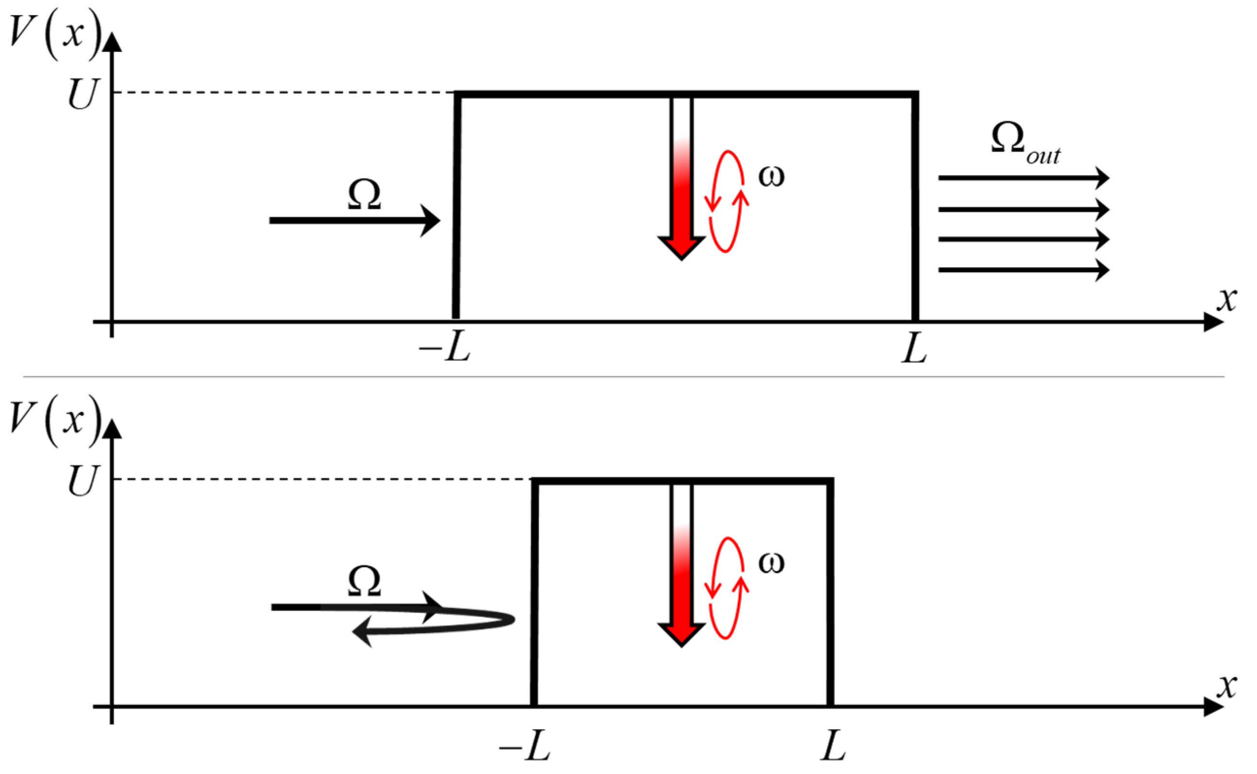
In the dynamic scenario, an oscillating component is added, and the Schrödinger equation reads:

$$-\frac{{\partial }^2}{\partial x^2}\mathsf{\psi }+U\left(x\right)\mathsf{\psi }+\left(\mathsf{\alpha }+\mathsf{\beta }\cos \mathsf{\omega }t\right)\mathsf{\delta }\left(x\right)\mathsf{\psi }=i\frac{\partial \mathsf{\psi }}{\partial t}$$

(7)

The dynamic system is illustrated in Figure 3.

The solution of Equation (7) can be written as a superposition of discrete energy expressions:

$$\mathsf{\psi }\left(x,t\right)=\{\begin{array}{cc}{\mathsf{\phi }}_0^{+}\exp \left(-i{\Omega }_{0}t\right)+{\displaystyle \sum _{n=-\infty }^{\infty }{r}_n{\mathsf{\phi }}_n^{-}\exp \left(-i{\Omega }_{n}t\right)}& x<0\\ {\displaystyle \sum _{n=-\infty }^{\infty }{t}_n{\mathsf{\phi }}_n^{+}\exp \left(-i{\Omega }_{n}t\right)}& x>0\end{array}$$

(8)

where ${\mathsf{\phi }}_n^{\pm }$ are the homogeneous solutions of waves that propagate from left to right $\left({\mathsf{\phi }}_n^{+}\right)$ and from right to left $\left({\mathsf{\phi }}_n^{-}\right)$, i.e.,

$${\mathsf{\phi }}_n^{+}\to {\tau }_{{\Omega }_n}\exp \left[i{k}_{n}x-i{\Omega }_{n}t\right]\hspace{1em}\left(for\hspace{0.17em}x\to \infty \right)$$

(9)

$${\mathsf{\phi }}_n^{-}\to {\tau }_{{\Omega }_n}\exp \left[-i{k}_{n}x-i{\Omega }_{n}t\right]\hspace{1em}\left(for\hspace{0.17em}x\to -\infty \right)$$

(10)

where $k_n=\sqrt{{\Omega }_n}$, ${\Omega }_n\equiv \Omega +n\mathsf{\omega }$. ${\left|{\tau }_{\Omega }\right|}^2$ is the probability of penetrating the stationary barrier with energy $\Omega$, and finally, $r_n$ and $t_n$ are the modes’ coefficients. It is worth noting the difference between the coefficients of the modes, i.e., $r_n$ and $t_n$, which need to be found, and the transmission coefficient of a single mode ${\tau }_{{\Omega }_n}$, which is obtained by solving the stationary case.

Using the boundary conditions at $x=0$:

$${\mathsf{\psi }}_l\left(0\right)={\mathsf{\psi }}_r\left(0\right)$$

(11)

$${{\mathsf{\psi }}^{\prime }}_l\left(0\right)-{{\mathsf{\psi }}^{\prime }}_r\left(0\right)=-\left(\mathsf{\alpha }+\mathsf{\beta }\cos \left(\mathsf{\omega }t\right)\right){\mathsf{\psi }}_r\left(0\right)$$

(12)

where the tags stand for spatial derivations.

The problem reduces to the following difference equation:

$$-{\chi }_n\mathsf{\delta }\left(n\right)=\left(\mathsf{\alpha }-{\chi }_n\right)s_n+\frac{\mathsf{\beta }}{2}\left(s_{n+1}+s_{n-1}\right)$$

(13)

where $s_n\equiv t_n\left({\mathsf{\phi }}_n^{+}/{\mathsf{\phi }}_0^{+}\right)$,

$${\chi }_n\equiv \frac{{\mathsf{\phi }}_n^{+}’}{{\mathsf{\phi }}_n^{+}}-\frac{{\mathsf{\phi }}_n^{-}’}{{\mathsf{\phi }}_n^{-}}=\frac{1}{G_n^{+}\left(0\right)}\equiv -2{\mathsf{\rho }}_n\tanh \left[{\mathsf{\rho }}_{n}L-i\arctan \left(k_n/{\mathsf{\rho }}_n\right)\right]$$

(14)

$G_n^{+}\left(0\right)\equiv G_{{\Omega }_n}^{+}\left(0\right)$ is the outgoing Green function of Equation (7) at x = 0 and ${\mathsf{\rho }}_n=\sqrt{U-{\Omega }_n}$.

Finally, the current through the barrier is:

$$j=2\Re {\displaystyle \sum _{n=-\infty }^{\infty }{\left|t_n\right|}^2{\left|{\tau }_n\right|}^2{k}_n}$$

(15)

where $\Re$ represents the real part.

The current Equation (15), as a function of the barrier’s width $L$, is presented in Figure 4 for a given incoming energy $\Omega$.

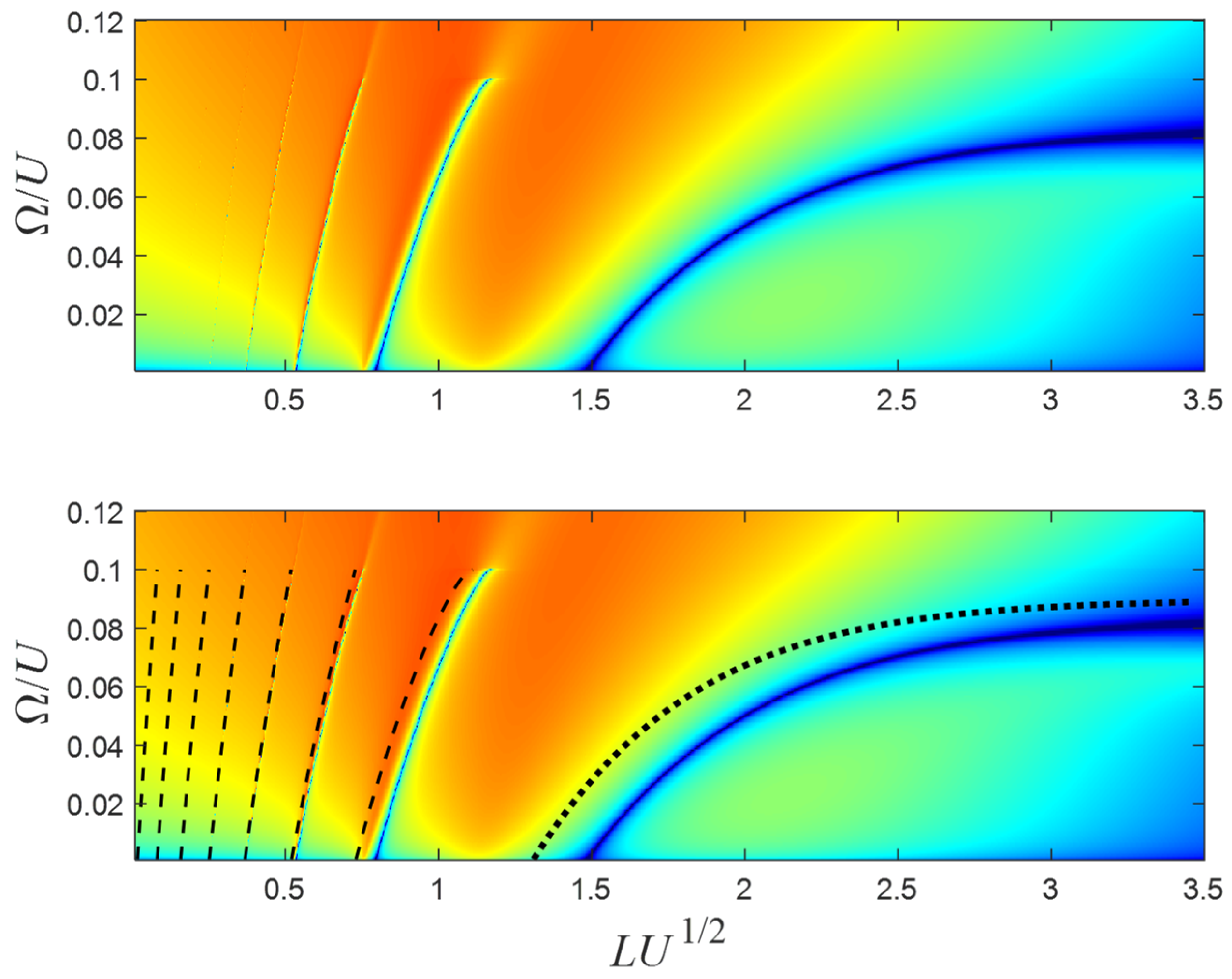
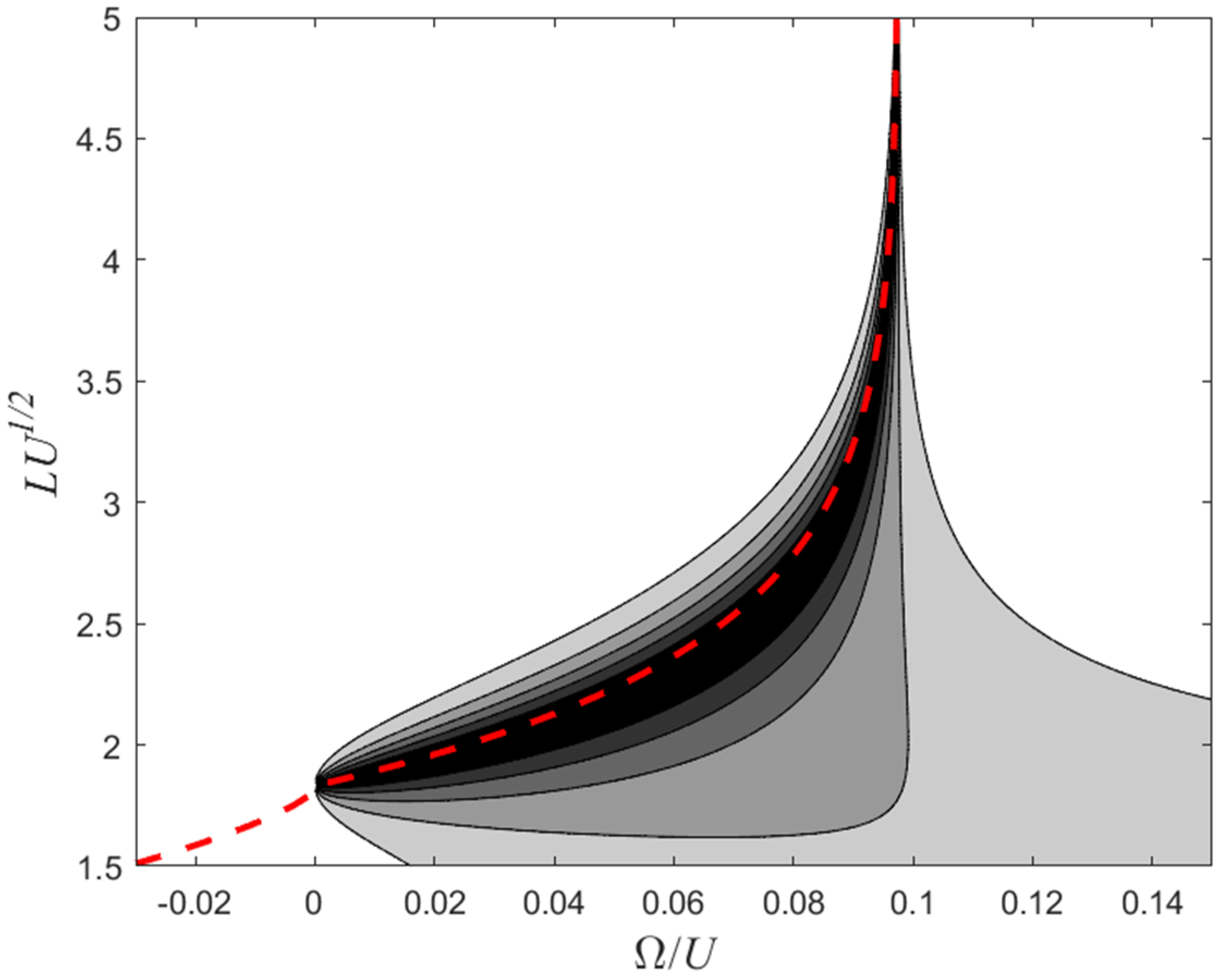
In Figure 5, the current is presented as a function of the particle’s incoming energy $\Omega$ and the barrier’s width $L$ for the same parameters as in Figure 4 (except $\Omega$). The red color represents a high current, while the blue color represents a low current.

As can be seen in Figure 4 and Figure 5, when the incident particle’s energy is lower than the oscillating energy $\Omega <\mathsf{\omega }$, multiple solutions of zero current exist, i.e., several Fano resonances appear for different values of $L$.

When the current is presented as a function of both $L$ and $\Omega$, the full structure of these Fano resonances appears. The narrower the barrier, the thinner the Fano resonances, and the lower the oscillation amplitude, the narrower the Fano resonances. Therefore, high-order resonances are very narrow and hard to detect. The zero currents are presented by the multiple curved lines. The zero-current curve (ZCC) on the right, i.e., for $L{U}^{1/2}>>1$, approximately agrees with Equation (5) for $L\left(\Omega -3\mathsf{\omega }\right)$. It should be noted that, since during the dynamic process, the instantaneous resonance energy varies in time, the resonance energy (Equation (4)) should be replaced with the minimum resonance energy, i.e.,

$${\Omega }_R\cong U-{\left(\left|\mathsf{\alpha }\right|+\mathsf{\beta }\right)}^2/4$$

(16)

Moreover, the other curves approximately agree with $L\left(\Omega -m\mathsf{\omega }\right)$ for $m=3,4\dots$. That is, these ZCCs can be regarded approximately as a folded curve. The curves cannot exceed the oscillating frequency $\Omega <\mathsf{\omega }$. The number of ZCCs (N) is finite, which can be evaluated by dividing the bare well’s (i.e., without the barrier) depth by the oscillating frequency $\mathsf{\omega }$, i.e., $N\cong {\mathsf{\alpha }}^2/4\mathsf{\omega }$. In the case presented in Figure 4 and Figure 5, indeed, $N\cong 8$.

Equation (5) can be used to distinguish between two scenarios. There are two regimes in which $L$ has a real value. In the first scenario, the REOB is negative, ${\Omega }_R<0$ (Equation (16)), in which case, a real solution exists, provided ${\Omega }_R-U<\Omega -n\mathsf{\omega }<{\Omega }_R$. In this scenario, the Fano resonance exists even for very opaque barriers, i.e., $L$ can be arbitrarily large. In the second scenario, the REOB is positive, $0<{\Omega }_R<U$, in which case, a real solution exists, provided ${\Omega }_R-U<\Omega -n\mathsf{\omega }<0$. In this scenario, Fano resonance exists only for finite-width barriers. Specifically, $L$ must be narrower than $L_0$ (Equation (6)).

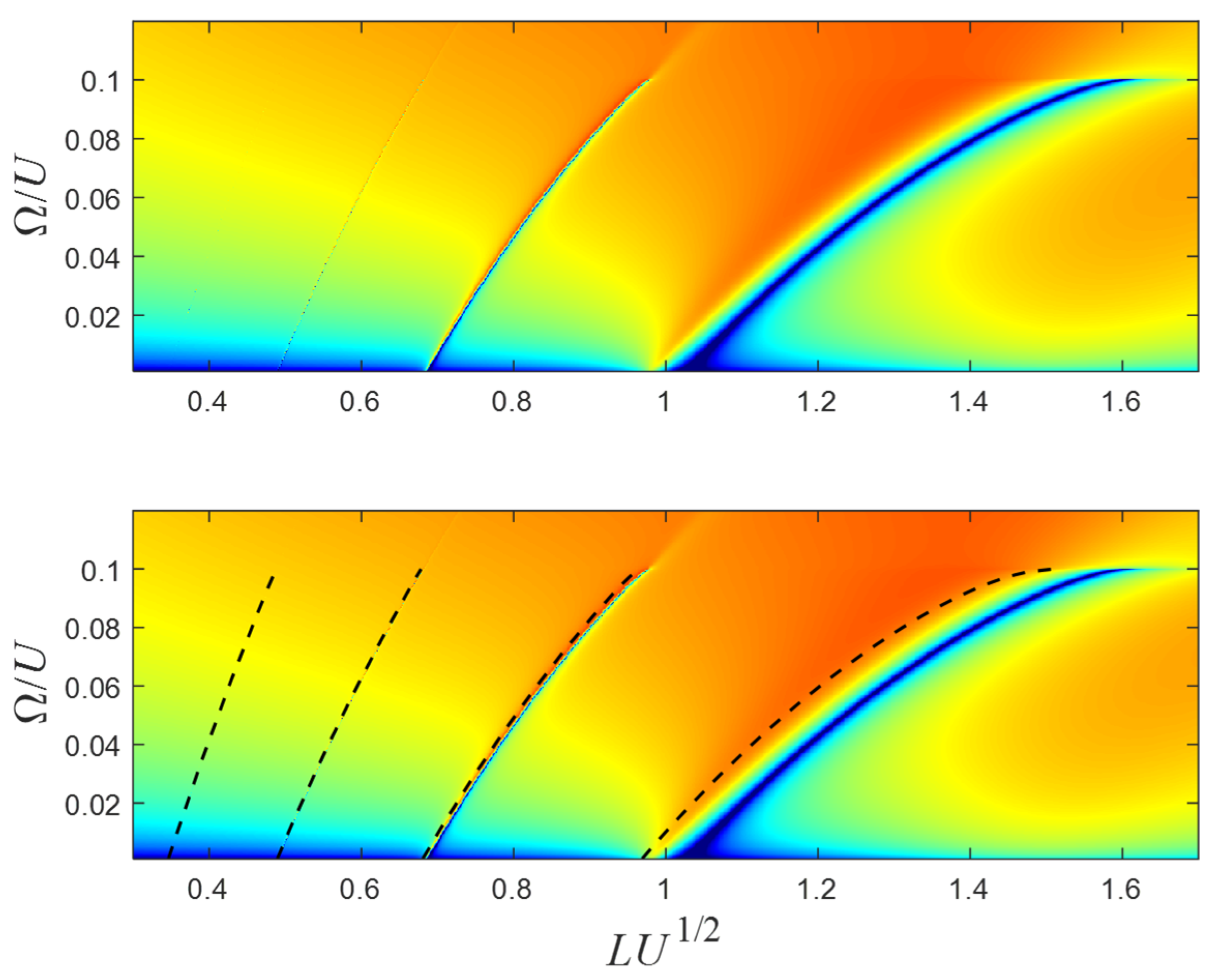
The second scenario is presented in Figure 6 and Figure 7. It can clearly be shown that, unless the barrier’s width is narrower than a certain cut-off value, no Fano resonances appear. In particular, this scenario does not support a Fano resonance (and hence no zero transmission) in the opaque barrier regime. The discrepancy between the cut-off value of the barrier’s width and $L_0$ (Equation (6)) is due to the fact that Equation (6) was calculated assuming $\mathsf{\beta }=0$. It will be shown that, when $\mathsf{\beta }$ is weak, there is an excellent agreement with Equation (6).

The multiple solutions of $L_n$ can be derived qualitatively by replacing $\Omega$ with $\Omega -n\mathsf{\omega }$ in Equation (5), yielding:

$$L_n\cong \frac{\mathrm{arctanh}\left(\sqrt{\frac{U-{\Omega }_R}{U-\Omega +n\mathsf{\omega }}}\right)-\mathrm{arctanh}\left(\sqrt{\frac{-\Omega +n\mathsf{\omega }}{U-\Omega +n\mathsf{\omega }}}\right)}{\sqrt{U-\Omega +n\mathsf{\omega }}}$$

(17)

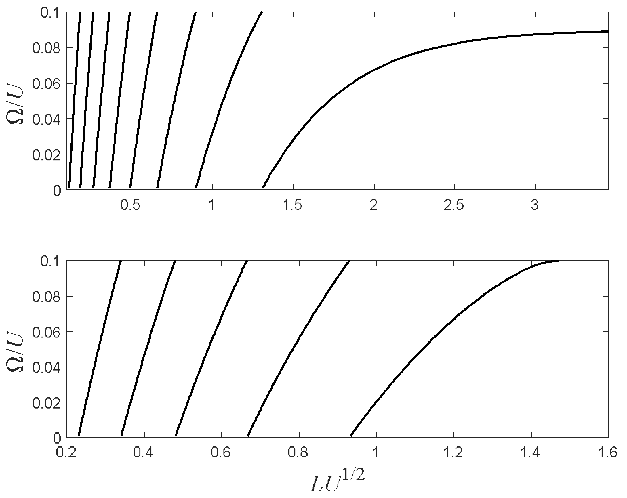
These solutions are plotted in Figure 8 for $0<\Omega <\mathsf{\omega }$ for two scenarios. It is worth noting the qualitative similarity between the upper/lower panels of Figure 8, and Figure 5/Figure 7, respectively. The folding nature of Equation (17) can be presented by the following relation:

$$L_n(\Omega )=L_0\left(\Omega -n\mathsf{\omega }\right)$$

(18)

4. Exact Numerical Solution and Approximate Analytical Solution for the Zero-Transmission Solution

Equation (13) can be rewritten in a matrix form $Mt=v$, where

$$M=\left(\begin{array}{ccccccc}\ddots & \ddots & & & & & \\ \ddots & \mathsf{\alpha }-{\chi }_{-2}& \mathsf{\beta }/2& & & & \\ & \mathsf{\beta }/2& \mathsf{\alpha }-{\chi }_{-1}& \mathsf{\beta }/2& & & \\ & & \mathsf{\beta }/2& \mathsf{\alpha }-{\chi }_0& \mathsf{\beta }/2& & \\ & & & \mathsf{\beta }/2& \mathsf{\alpha }-{\chi }_1& \mathsf{\beta }/2& \\ & & & & \mathsf{\beta }/2& \mathsf{\alpha }-{\chi }_2& \ddots \\ & & & & & \ddots & \ddots \end{array}\right)\hspace{0.17em} \mathrm{and} v=\left(\begin{array}{c}⋮\\ 0\\ 0\\ -{\chi }_0\\ 0\\ 0\\ ⋮\end{array}\right)$$

(19)

and ${\chi }_n\equiv -2{\mathsf{\rho }}_n\tanh \left[{\mathsf{\rho }}_{n}L-i\arctan \left(k_n/{\mathsf{\rho }}_n\right)\right]$ (Equation (14)).

Let us further define

$$M_{\left(-1\right)}^{\left(-N\right)}=\left(\begin{array}{ccccc}\mathsf{\alpha }-{\chi }_{-N}& \mathsf{\beta }/2& & & \\ \mathsf{\beta }/2& \ddots & \ddots & & \\ & \ddots & & \mathsf{\beta }/2& \\ & & \mathsf{\beta }/2& \mathsf{\alpha }-{\chi }_{-2}& \mathsf{\beta }/2\\ & & & \mathsf{\beta }/2& \mathsf{\alpha }-{\chi }_{-1}\end{array}\right)$$

(20)

and

$$M_{\left(N\right)}^{\left(1\right)}=\left(\begin{array}{ccccc}\mathsf{\alpha }-{\chi }_1& \mathsf{\beta }/2& & & \\ \mathsf{\beta }/2& \mathsf{\alpha }-{\chi }_2& \mathsf{\beta }/2& & \\ & \mathsf{\beta }/2& \ddots & \ddots & \\ & & \ddots & & \mathsf{\beta }/2\\ & & & \mathsf{\beta }/2& \mathsf{\alpha }-{\chi }_N\end{array}\right)$$

(21)

Then, the solution of the zero mode $t_0$ reads (for details see ref. [34]),

$$t_0=-{\chi }_0\underset{N\to \infty }{\lim }\frac{\left|M_{\left(-1\right)}^{\left(-N\right)}\right|\left|M_{\left(N\right)}^{\left(1\right)}\right|}{\left|M_0^{\left(N\right)}\right|}$$

(22)

Therefore, zero transmission is reached when

$$\left|M_{\left(-1\right)}^{\left(-N\right)}\right|=0$$

(23)

It follows from Equation (11) and current conservation that, when Equation (22) vanishes, the current must vanish as well. Therefore, the solution of Equation (23) corresponds to the multiple solutions for which the current vanishes.

For any given energy, several solutions exist for different values of $L$. Nevertheless, we can straightforwardly deduce that Equation (23) is valid, provided that the incoming particle’s energy is lower than the oscillating frequency, i.e., $\Omega <\mathsf{\omega }$. Otherwise, some of the $k_{-m}$ (for 1 < m < N) are real, and if this is the case, then the term

${\chi }_{-m}=-2{\mathsf{\rho }}_{-m}\tanh \left[{\mathsf{\rho }}_{-m}L-i\arctan \left(k_{-m}/{\mathsf{\rho }}_{-m}\right)\right]$ (Equation (14)) (which are the only elements in the matrix (20) that can have imaginary components) is not necessarily real (noting that all the ${\mathsf{\rho }}_{-m}$ terms are real). Consequently, the determinant is not real and cannot vanish. This fact is consistent with the fact that the Fano resonances are limited by $\Omega <\mathsf{\omega }$, and with the folding nature of the periodicity, a 2D map structure qualitatively similar to Figure 8 appears.

5. Weak Modulation Regime

In the weak modulation amplitude ($\mathsf{\beta }$) regime at the vicinity of $\mathsf{\alpha }\cong {\chi }_{-m}$, the determinant of (20) can be written as approximately:

$$\left|M_{\left(-1\right)}^{\left(-N\right)}\right|=\left(\mathsf{\alpha }-{\chi }_{-m}\right)\left|M_{\left(-m-1\right)}^{\left(-N\right)}\right|\left|M_{\left(-1\right)}^{\left(-m+1\right)}\right|-\frac{{\mathsf{\beta }}^2}{4}\left(\left|M_{\left(-m-1\right)}^{\left(-N\right)}\right|\left|M_{\left(-1\right)}^{\left(-m+2\right)}\right|+\left|M_{\left(-m-2\right)}^{\left(-N\right)}\right|\left|M_{\left(-1\right)}^{\left(-m+1\right)}\right|\right)+O\left({\mathsf{\beta }}^4\right)$$

(24)

which can also be rewritten as:

$$\left|M_{\left(-1\right)}^{\left(-N\right)}\right|\cong {\displaystyle \prod _{m^{\prime }=1}^N\left(\mathsf{\alpha }-{\chi }_{-m^{\prime }}\right)\left[1-\frac{{\mathsf{\beta }}^2}{4}\frac{1}{\left(\mathsf{\alpha }-{\chi }_{-m}\right)}\left(\frac{1}{\left(\mathsf{\alpha }-{\chi }_{-m-1}\right)}+\frac{1}{\left(\mathsf{\alpha }-{\chi }_{-m+1}\right)}\right)+O\left({\mathsf{\beta }}^4\right)\right]}$$

(25)

Therefore, the transmission vanishes (Equation (23) is valid) up to the second order in $\mathsf{\beta }$, provided that:

$$1\cong \frac{{\mathsf{\beta }}^2}{4}\frac{1}{\left(\mathsf{\alpha }-{\chi }_{-m}\right)}\left(\frac{1}{\left(\mathsf{\alpha }-{\chi }_{-m-1}\right)}+\frac{1}{\left(\mathsf{\alpha }-{\chi }_{-m+1}\right)}\right)$$

(26)

Since ${\chi }_n$ is a function of $L$, one can find an expression for the relation between the zero-transmission energy $\Omega$ and the width of the barrier $L$:

$$L_m(\Omega )\cong \frac{\mathrm{arctanh}\left\{\frac{1}{2{\mathsf{\rho }}_{-m}}\left[\frac{{\mathsf{\beta }}^2}{8i}\left(\frac{1}{\left(k_{-m}-k_{-m-1}\right)}+\frac{1}{\left(k_{-m}-k_{-m+1}\right)}\right)-\mathsf{\alpha }\right]\right\}+i\arctan \left(\frac{k_{-m}}{{\mathsf{\rho }}_{-m}}\right)}{{\mathsf{\rho }}_{-m}}$$

(27)

In the regime where the barrier is opaque, i.e., $L{U}^{1/2}>>1$, Equation (27) can be approximated by:

$\left(\mathsf{\alpha }+2{\mathsf{\rho }}_{-1}\right)\cong \frac{1}{\left(\mathsf{\alpha }+2{\mathsf{\rho }}_{-2}\right)}{\left(\frac{\mathsf{\beta }}{2}\right)}^2$, and when $\mathsf{\beta }<<\mathsf{\alpha }$, it can be solved for the energy:

$${\Omega }_c\cong U+\mathsf{\omega }-\frac{1}{4}{\left[\mathsf{\alpha }-\frac{{\left(\mathsf{\beta }/2\right)}^2}{\mathsf{\alpha }+2\sqrt{\mathsf{\omega }+{\mathsf{\alpha }}^2/4}}\right]}^2$$

(28)

Expression (27) is presented in Figure 4, Figure 5, Figure 6 and Figure 7. The discrepancy between this expression and the numerical results, which is larger for low orders, is due to the fact that Equation (27) is derived for a weak $\mathsf{\beta }$. In the following Figure 9, Figure 10, Figure 11 and Figure 12, since $\mathsf{\beta }$ is smaller, there is a better agreement with Equation (27).

In Figure 9 and Figure 10, the second scenario (i.e., $0<{\Omega }_R<U$) is presented for a weak $\mathsf{\beta }$. In Figure 11 and Figure 12, the first scenario (i.e., ${\Omega }_R<0$) is presented for a weak $\mathsf{\beta }$. As can be seen in both cases, the agreement with the theoretical prediction (Equation (27)) is excellent.

6. Narrow Barrier Regime

In the narrow barrier regime, i.e., when the width of the barrier is considerably narrower than the incoming particle’s wavelength, Equation (26) can be rewritten as:

$$1\cong \frac{{\mathsf{\beta }}^2}{4}\frac{1}{\left({\mathsf{\alpha }}_0-{\chi }_{-m}\right)}\left(\frac{1}{\left({\mathsf{\alpha }}_0-{\chi }_{-m-1}\right)}+\frac{1}{\left({\mathsf{\alpha }}_0-{\chi }_{-m+1}\right)}\right)$$

(29)

where ${\mathsf{\alpha }}_0=\mathsf{\alpha }+UL$. In which case, $\Omega \cong m\mathsf{\omega }-\frac{{\mathsf{\alpha }}_0^2}{4}-\frac{{\mathsf{\beta }}^2}{8}$, or equivalently:

$$\Omega \cong m\mathsf{\omega }-\frac{{\left(\mathsf{\alpha }+U{L}_m\right)}^2}{4}-\frac{{\mathsf{\beta }}^2}{8}$$

(30)

This expression relates the different barrier widths $L_m$, which yield Fano resonances, to the same energy $\Omega$. In what follows, we will investigate the implications of this.

7. Strong Oscillations and Opaque Barrier Regime

In the wide barrier regime, i.e., when the barrier is opaque, the dependence of the resonance energy on the barrier’s width $L$ is exponentially small and can therefore be neglected. Furthermore, in this regime, the particle is approximately trapped in the well and the QBSS is well defined. It has been shown that the transmission via this state is extremely sensitive to the incoming particle’s energy ($\Omega$). For some values of $\Omega$, which are consistent with the spectral component of the QBSS, the QBSS is highly excited and, consequently, the tunneling current is very high. Similarly, for other energy values, which are inconsistent with the spectral components of the QBSS, the particle cannot be trapped and the tunneling current is highly suppressed. These scenarios have been well investigated [10,14,18]. In particular, it has been found that current suppression occurs for the energies:

$${\displaystyle \underset{t_1}{\overset{t_2}{\int }}\left(\Omega -{\Omega }_R\left(t\prime \right)\right)}dt\prime =\left(m-\frac{1}{4}\right)\pi$$

(31)

where, for the case under study, i.e., Equation (7),

$${\Omega }_R\left(t\right)=U-\frac{{\left(\mathsf{\alpha }+\mathsf{\beta }\cos \left(\mathsf{\omega }t\right)\right)}^2}{4}$$

(32)

is the instantaneous resonance energy of the well and $t_1$ and $t_2$ are the solutions of $\Omega ={\Omega }_R\left(t\right)$ [10,14,18], i.e., these are the instances in which the incoming particle’s energy coincides with the instantaneous resonant state’s energy. The solutions of (31) for the case (32) are:

$${\Omega }_m\cong U-\left(\frac{{\mathsf{\alpha }}^2}{4}+\frac{{\mathsf{\beta }}^2}{8}\right)-\left[\frac{\left|\mathsf{\alpha }\right|\mathsf{\beta }}{\pi }-2\mathsf{\omega }\left(m-\frac{1}{4}\right)\right]$$

(33)

Similarly, for a given incoming energy, the oscillating amplitudes, which correspond to the current suppression, are:

$${\mathsf{\beta }}_m=-\frac{4\left|\mathsf{\alpha }\right|}{\pi }+\sqrt{\frac{16{\mathsf{\alpha }}^2}{{\pi }^2}+8\left(U-\Omega -\frac{{\mathsf{\alpha }}^2}{4}+2\mathsf{\omega }\left(m-\frac{1}{4}\right)\right)}$$

(34)

However, although this expression has been found to be in good agreement with numerical simulations, it only predicts current suppression. It does not predict zero current. The reason for this is that, as has been explained in refs. [10,11], at the suppression energies, only the upper half of the spectrum (${\Omega }_{out}\ge {\Omega }_{in}$) is suppressed. Therefore, in a case where the incoming energy is higher than the oscillating frequency $\Omega >\mathsf{\omega }$, the lower part of the spectrum still includes propagating modes, since the particle can lose a quantum $\mathsf{\omega }$ and still escape from the well. To prevent this, the existence of a Fano resonance (and zero transmission) requires the additional condition (additional to (31)) that $\Omega <\mathsf{\omega }$, in which case, the output spectrum consists of only negative energies. Therefore, positive energies cannot propagate and the incoming particles are completely reflected. This required additional condition is consistent with the explanation that follows Equation (23). The difference between these two kinds of suppressions (low current vs. zero current) is illustrated in Figure 13, where the current, as a function of the incoming energy $\Omega$ and a function of the oscillation amplitude $\mathsf{\beta }$, is presented. When the incoming energies are lower than the oscillation frequency $\Omega <\mathsf{\omega }$, a total reflection appears for appropriate amplitudes. In the lower panel, the analytical results of Equation (33) are presented by dashed black curves above the numerical results. The analytical results represent suppression scenarios; however, the suppressions’ characteristics are fundamentally different in the regions $\Omega <\mathsf{\omega }$ and $\Omega >\mathsf{\omega }$. In the region $\Omega <\mathsf{\omega }$, the suppression manifests in 100% reflection, whereas in the region $\Omega >\mathsf{\omega }$, the current suppression is substantial, albeit not entirely zero.

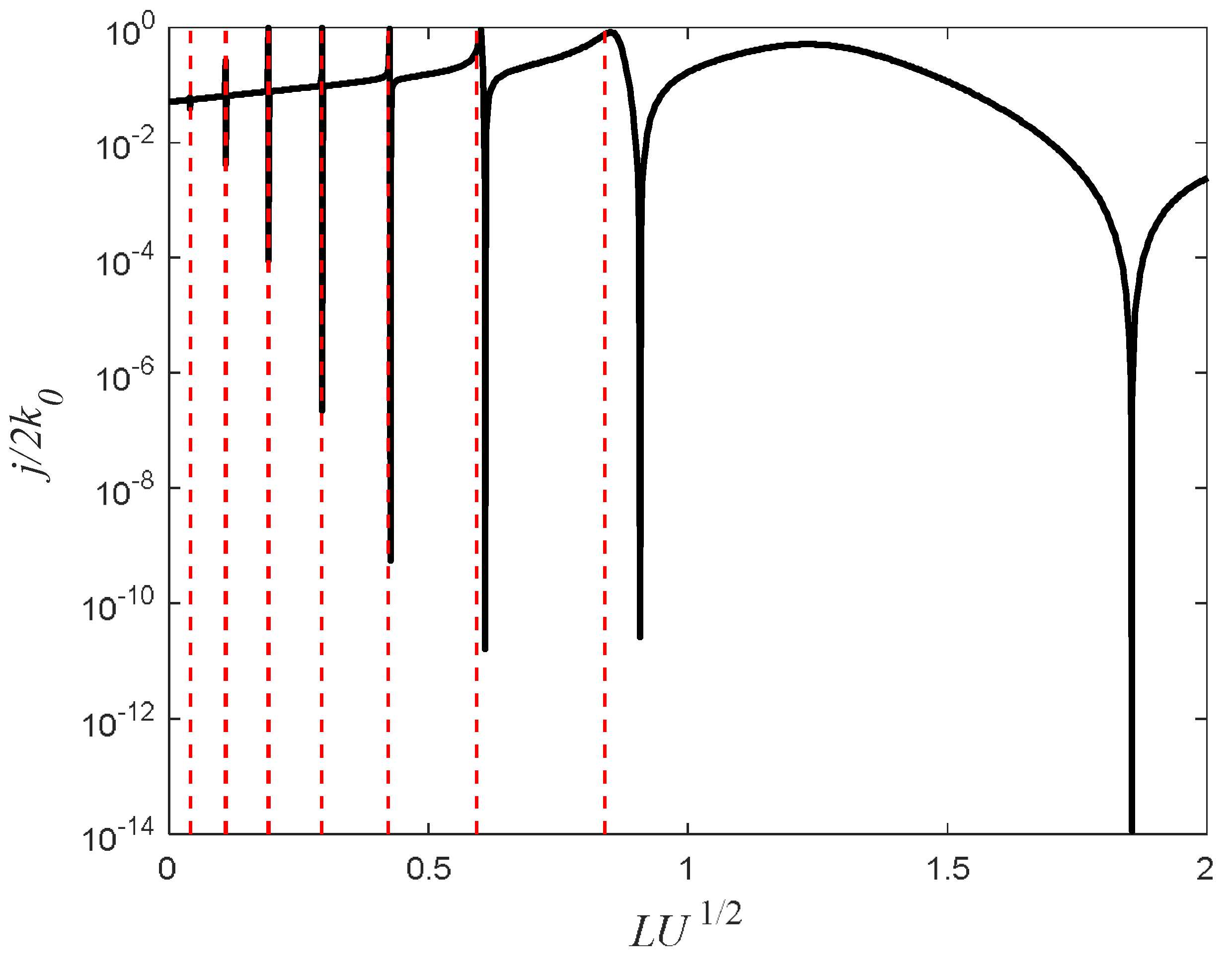
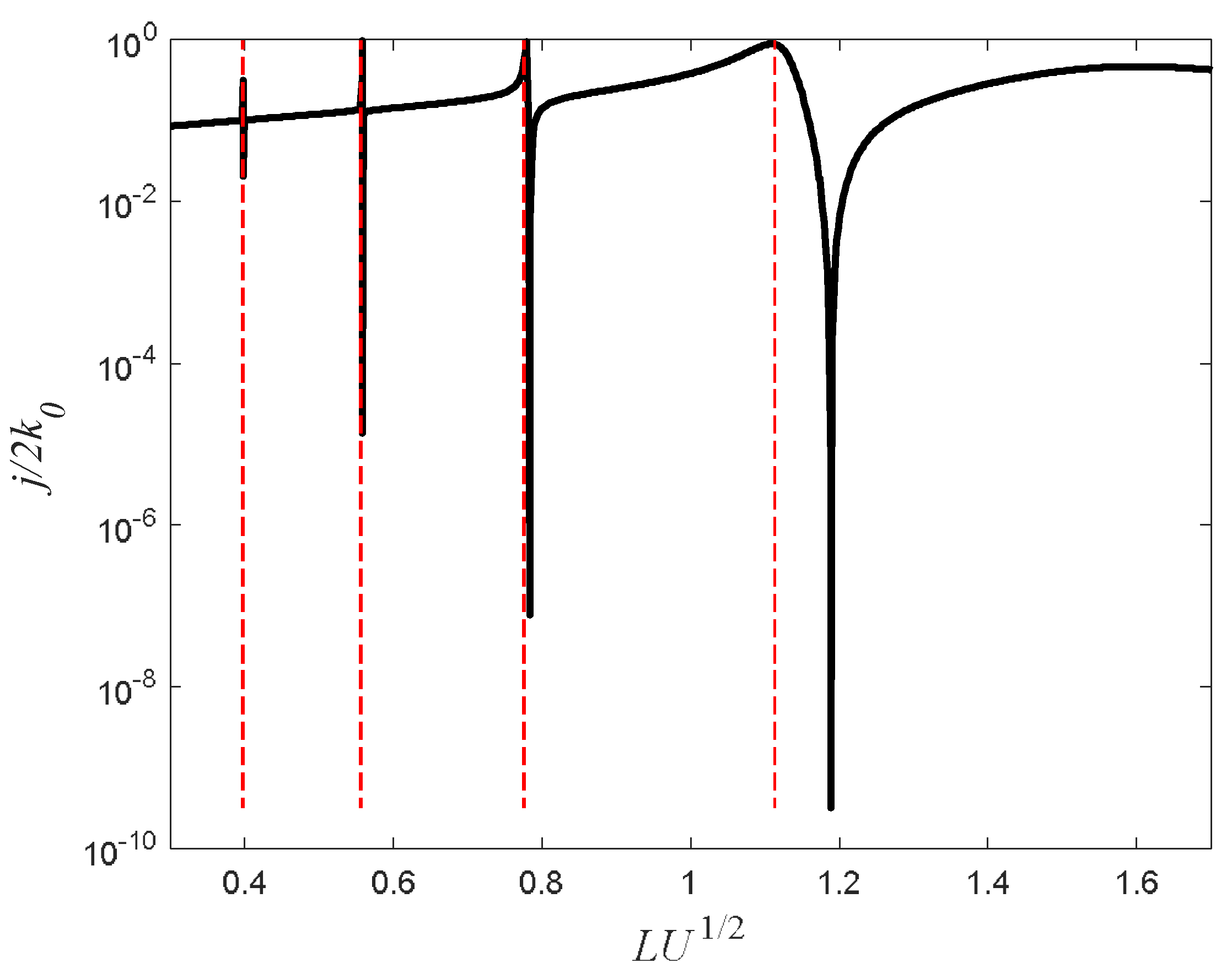
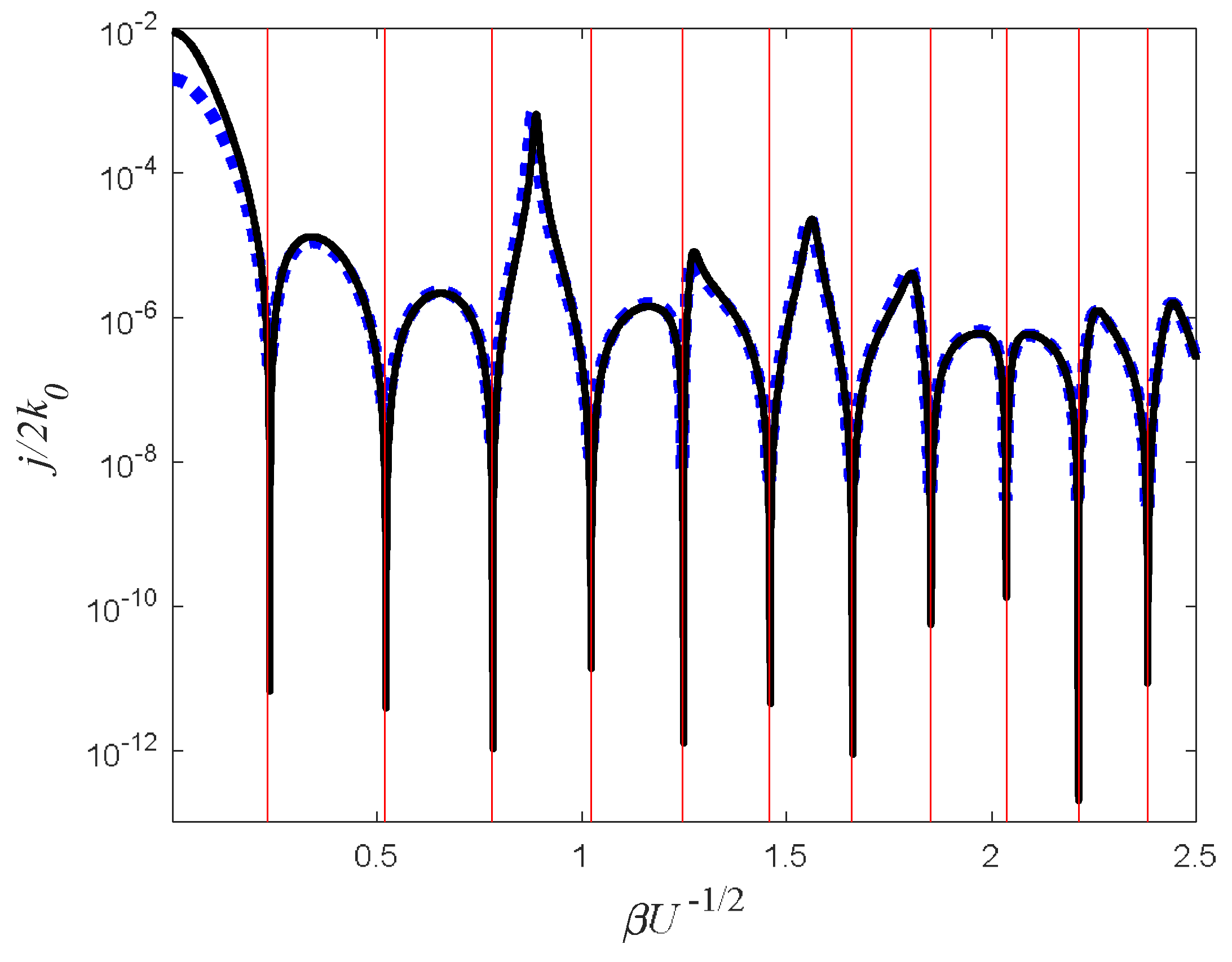
Figure 14 illustrates the difference between the two regimes. The current is plotted as a function of the oscillation amplitudes for two adjacent incoming energies. One of the energies is slightly lower than the oscillation frequency $\mathsf{\omega }$ and the other is slightly higher than the oscillation frequency. Although the two plots look alike, they are fundamentally different. When $\Omega /\mathsf{\omega }=0.99$, the minima are exactly zero, while, when $\Omega /\mathsf{\omega }=1.01$, the suppression is indeed substantial, but does not go to zero. Moreover, as can be seen with the vertical red lines, the analytical expression of the suppression amplitude ${\mathsf{\beta }}_m$ (Equation (34)) agrees with the numerical results.

8. High Precision Interferometry

When an object is measured with a wave beam, then usually, the shorter the wavelength, the better the resolution. In the case of a simple rectangular barrier, the interference between the reflections from its boundaries determines the dynamic range of the measurement. Therefore, if a small object with dimensions $~\Delta L$ is measured, then, unless the particle’s frequency is of the order $~\Delta L^{-2}$, the dynamic range would be minuscule and of the order of ${\left(\Delta L/\lambda \right)}^2\ll 1$, where $\lambda$ is the particle’s de-Broglie wavelength.

Ref. [18] suggested fabricating a quantum device like the one presented in Equation (7) and Figure 3 as a frequency-controlled quantum transistor. The oscillations can be confined in space using well-known technology (see, for example, ref. [35]). The present work teaches that the dynamic range of these devices can be increased substantially.

The Fano nature of these resonances shows that the dynamic range is almost 100%, regardless of the barrier’s width and oscillating frequency.

In the case where the oscillating part (width $\mathsf{\epsilon }$ and height $V$) and measured object (width $L$ and height $U$) are very narrow in comparison to the incoming particle’s wavelength, Equation (30) can be simplified to (since now ${\mathsf{\alpha }}_0\cong V\mathsf{\epsilon }$):

$$\Omega \cong m\mathsf{\omega }-\frac{{\left(V\mathsf{\epsilon }+U{L}_m\right)}^2}{4}-\frac{{\mathsf{\beta }}^2}{8}$$

(35)

This equation can be rewritten as:

$$\Omega \cong \left[-\frac{{\left(V\mathsf{\epsilon }+U{L}_m\right)}^2}{4}-\frac{{\mathsf{\beta }}^2}{8}\right]\mathrm{mod}\mathsf{\omega }$$

(36)

where $\mathrm{mod}$ represents the modulo operation.

In the case where ${\mathsf{\alpha }}_0>>U{L}_m$, then the widths $L_m$, for which zero transmission is reached, must maintain:

$$\Omega \cong m\mathsf{\omega }-\frac{{\mathsf{\alpha }}_0^2+2{\mathsf{\alpha }}_{0}U{L}_m}{4}-\frac{{\mathsf{\beta }}^2}{8}$$

(37)

Therefore, the difference between the adjacent widths is $L_m-L_{m+1}=\Delta L\cong \frac{2\mathsf{\omega }}{{\mathsf{\alpha }}_{0}U}$. Or, equivalently, a change $\mathsf{\delta }L$ in the barrier’s width will change the zero-transmission energy by:

$$\Delta \Omega \cong \frac{V\mathsf{\epsilon }U}{2}\mathsf{\delta }L$$

(38)

In real physical units, Equation (38) can be written as $\Delta \Omega \cong \frac{m}{{\hslash }^3}VU\mathsf{\epsilon }\mathsf{\delta }L$, where m represents the effective mass in the material, which, for GaAs (where the effective mass is 0.067 times the mass of the free electron [35]), Equation (38) can therefore be written as:

$$\Delta \Omega \left[\mathrm{Hz}\right]\cong 1.5\times {10}^{15}VU\mathsf{\epsilon }\mathsf{\delta }L$$

(39)

In Equation (39), the potential heights $V$ and $U$ are measured in eV and their widths $\mathsf{\epsilon }$ and $\mathsf{\delta }L$ are measured in nanometers. The change in the frequency is measured in Hz.

Therefore, if the oscillating part and measured object have a potential of ~0.01 eV and a width of ~1 nm, then every change of 0.01 nm ($0.1 \mathrm{A} \text{˙}$) varies the zero-transmission frequency by more than 1.5 GHz. Clearly, this result is valid, provided that the oscillating frequency is higher than this value. These values are easily achievable using contemporary electronics. Since the frequency can be measured with great accuracy, this device can exhibit an extremely high precision. Furthermore, unlike ordinary measurements, as was described at the beginning of this section, where high energy is required to achieve a high precision, such a requirement is not necessary and does not limit the performance of this device, which can operate in low energies.

Furthermore, since the measurement is taken where the current is zero, this device is highly resilient against different kinds of noises, especially shot noise, which should vanish at these points, thus having a negligible effect on the measurement. The presence of thermal noise (which can be reduced by lowering the temperature) would require more extended measurement periods (for averaging), in which case, a minimum current should be sought instead of a zero current, but Equation (39) should still be valid.

Such a device can be applied in several configurations. It can be used as a highly sensitive frequency-controlled transistor, where minuscule variations in the frequency can change the current drastically, or alternatively, it can be used as a high-precision measurement device for measuring nanostructures’ dimensions with sub-nanometer precision.

9. Conclusions and Summary

The tunneling current through a barrier via an oscillating well was investigated both numerically and analytically. While previous works have focused on the difference between high transmission (activation) and low transmission (current suppression), this work focused on the difference between current suppression and zero transmission. Since zero transmission is equivalent to a Fano resonance, it requires interference with a bound state. The following are the main conclusions:

(A)

A bound state can exist even when the well’s bound state is smaller (in absolute terms) than the height of the barrier (${\mathsf{\alpha }}^2/4<U$), and an analytical expression was derived to relate the resonance state to the barrier’s width $L\left({\Omega }_R\right)$. It was shown that the resonance state decreases when the barrier’s width shrinks. Therefore, if the barrier is narrow enough, the resonance state would eventually turn into a bound state.

(B)

When an oscillating term is introduced, it was shown that zero transmission (and therefore zero current) requires the incoming particle’s energy to be lower than the oscillating energy, i.e., $\Omega <\mathsf{\omega }$.

(C)

Since the particle can gain/lose oscillating quanta, for any given incoming energy, multiple solutions of the barrier’s width exist, and from (A) and (B), it follows that the solution curve is folded. Therefore, the solutions can be retrieved qualitatively: $L_n(\Omega )=L_0\left(\Omega -n\mathsf{\omega }\right)$.

(D)

It was found that there are two different scenarios:

(1)

When the Resonance Energy of the Opaque Barrier (REOB) is negative. In this scenario, the Fano resonance (zero transmission) occurs even for an infinitely wide barrier.

(2)

When the REOB is positive, the barrier must be narrower than a certain value for a Fano resonance to appear.

(E)

An analytical expression was derived for the barrier’s width, which supports Fano resonances $L_m(\Omega )$ up to the second order in the oscillation amplitude ${\mathsf{\beta }}^2$, and it was found to be in high agreement with exact numerical results.

(F)

In the case where the oscillation amplitude is large, one can use the method that was applied to the Sisyphus effect and the QBSS method [14,17], along with the additional requirement of $\Omega <\mathsf{\omega }$, calculating the Fano criteria with a high agreement with numerical simulations.

(G)

Finally, it was shown that, in the case of a very narrow barrier, a simple analytical expression relates the zero-transmission energy to the multiple barrier widths $L_n(\Omega )$, which support the Fano resonance. This expression shows that the energy, which can easily be measured, is extremely sensitive to the barrier’s width, and can therefore be used for high-precision measurements.