


A Novel Convolutional Neural Network Algorithm for Histopathological Lung Cancer Detection


Abstract
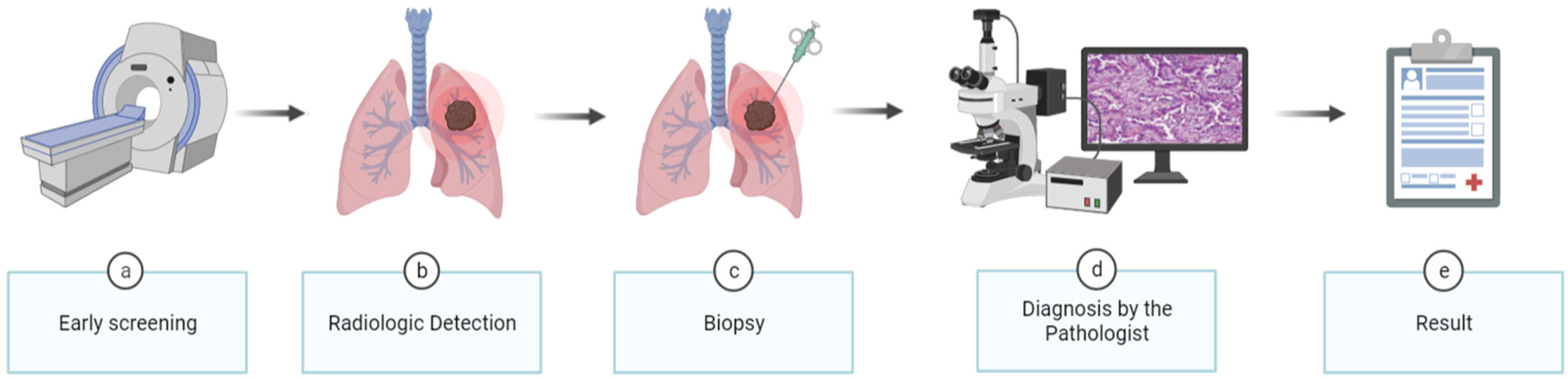
1. Introduction
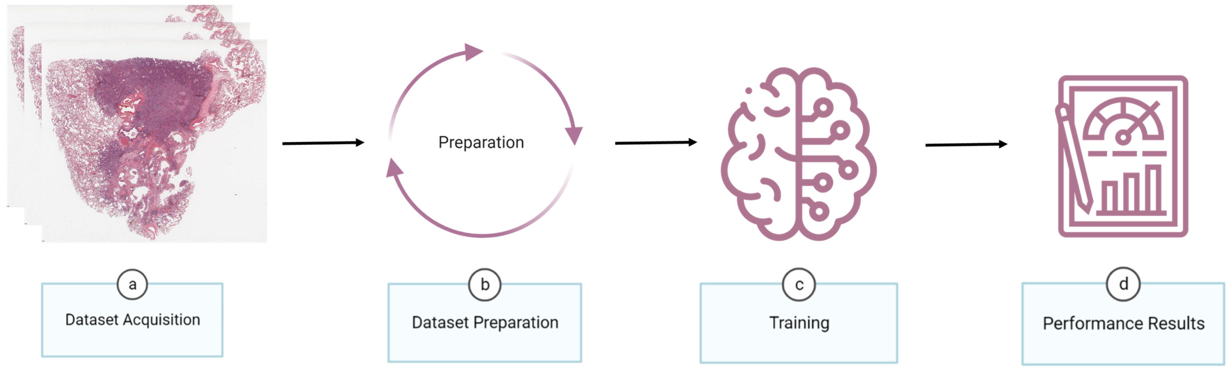
2. Materials and Methods
2.1. Dataset Acquisition
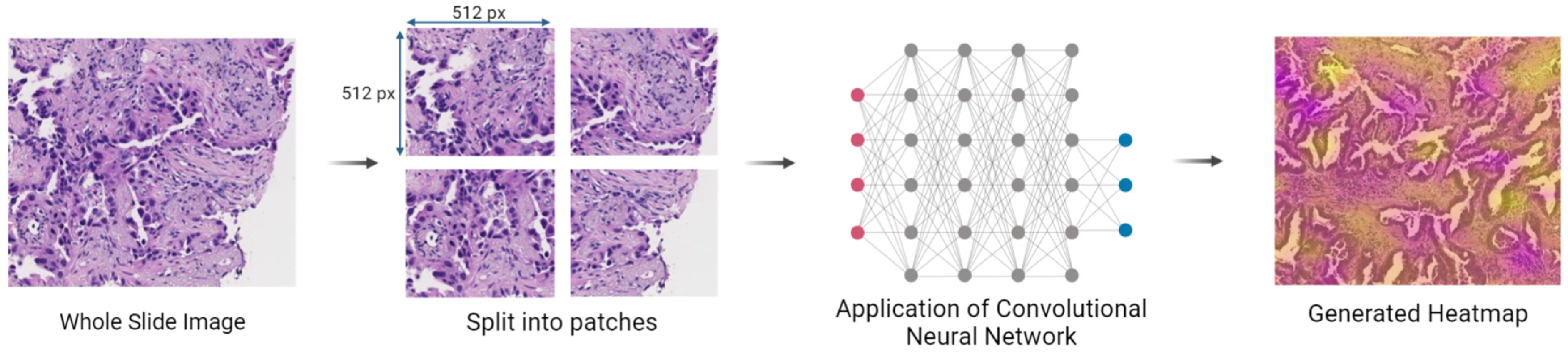
2.2. Dataset Preparation
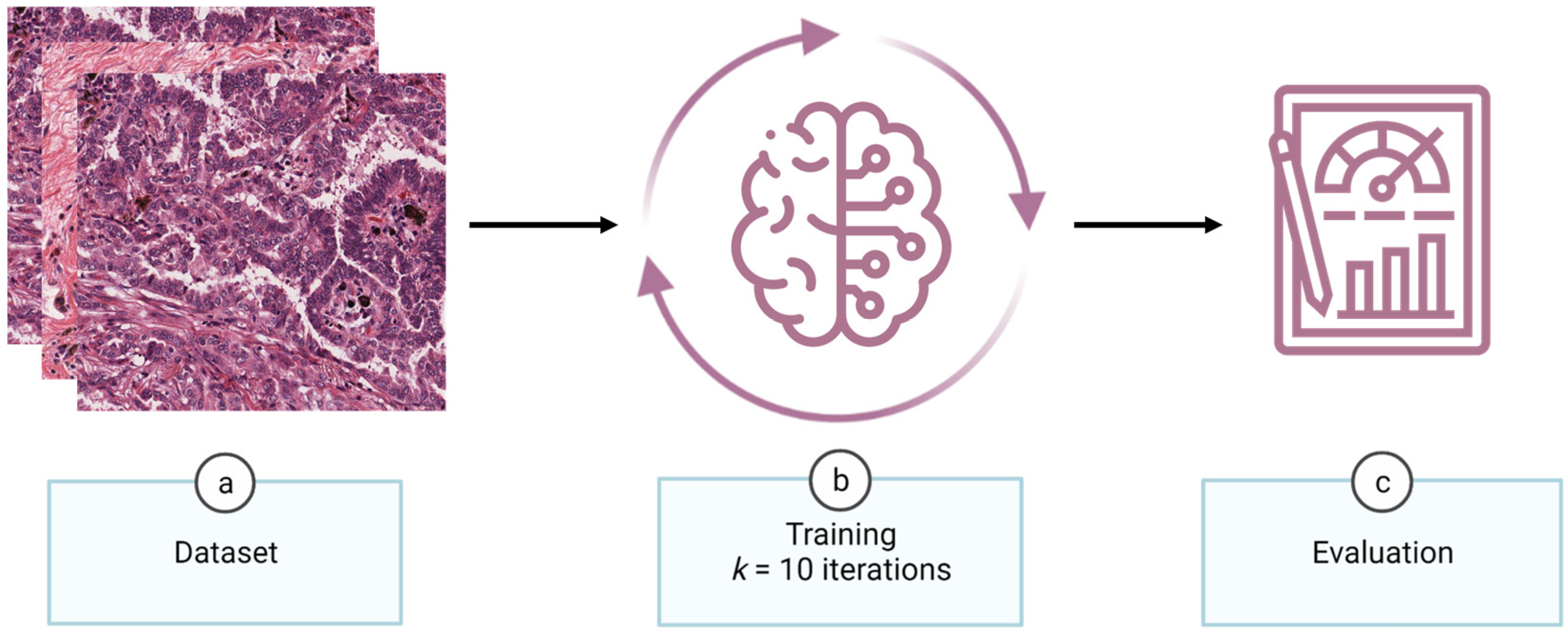
2.3. Training
2.3.1. Neural Networks
- Version 0: Composed of 3 layers, the model has the input dimensions set as 512 × 512 × 3 pixels. It starts with a convolution layer with a 3 × 3 pixels kernel size, 32 filters, 2 × 2 pixels strides, and the activation function is the rectified linear unit (ReLU). Then, there is a global average pooling layer followed by a fully connected layer of 1 unit employing the sigmoid activation function;
- Version 1: Introduced a fully connected layer with 512 units and ReLU as an activation function between global average pooling and fully connected layers of Version 0, in order to increase the model’s capacity to capture more complex patterns;
- Version 2: To reduce the dimensionality of the feature maps and enable the learning of more features, a max pooling layer with a pooling size of 2 × 2 pixels was added after the initial convolutional layer. Upon the addition of the new max pooling layer, a new set of convolution and max pooling layers were added, duplicating the identical dimensions and activation functions but with 64 filters rather than 32 in the convolution layer, which allows for learning more complicated features;
- Version 3: After the appended layers in Version 2, a new pair of convolution and max pooling layers were added, with the convolution layer having 128 filters. The increase in the number of filters makes the model more capable of acquiring more information about features and patterns;
- Version 4: Replicated the addition of Version 3;
- Version 5: The max pooling layer positioned before the global average pooling layer was removed to allow keeping more spatial information before the final classification;
- Version 6: The number of filters for the final convolution layer was increased to 256 to enhance the model’s ability to capture more complex features and patterns;
- Version 7: Contrary to the change made in Version 5, the max pooling layer placed before the global average pooling layer was reinserted with a size of 2 × 2 pixels, in order to downsample the spatial dimensions of the feature maps;
- Version 8: Placed a new set of convolution and max pooling layers before the global average pooling layer, one of which included 128 filters, and modified the first fully connected layer units from 512 to 128. While the reduction of units in the fully connected layer reduces the number of parameters and prevents overfitting, the addition of the convolutional layers increases the model’s capacity to learn more features, as described above;
- Version 9: Demonstrated a “U-architecture,” which means it has pairs of convolution layers and max pooling with only the filters changing in the following order: 32–64–128–256–128–64–32. This version also reduced the number of the first fully connected layer units from 128 to 32. The reasons for the changes remain the same as in the above versions;
- Version 10: Reverted the number of units in the first fully connected layer to 512 with the aim of capturing complex patterns;
- Version 11: Removed the previously added sets in Version 9 and changed the convolution layer from 256 to 128 filters. As a result, convolutional layers of 32, 64, and 128 filters were retained, culminating in a CNN with one convolution layer of 32 filters, another of 64 filters, and three of 128 filters. These changes simplified the CNN by reducing its parameters;
- Version 12: Deleted the last set of convolutional layers with 128 filters and max pooling layers, as well as the fully connected layer with 512 units, which reduces the number of parameters, helps prevent overfitting, and makes the model more computationally efficient.
2.3.2. Performance Metrics
- Accuracy, which measures the proportion of correct classifications over the total number of classifications [36]:
- Precision (or Specificity), which measures the proportion of true positive predictions over the total number of positive predictions [36]:
- Recall (or Sensitivity), which measures the proportion of true positive predictions over the total number of actual positive samples [36]:
- F1-score, which measures a weighted mean of Precision and Recall [36]:
- AUC, which measures the performance of a binary classifier by calculating the area under the receiver operating characteristic (ROC) curve and plotting the true positive rate against the false positive rate at various classification thresholds [36]:
2.3.3. k-Fold Cross-Validation
3. Results and Discussion
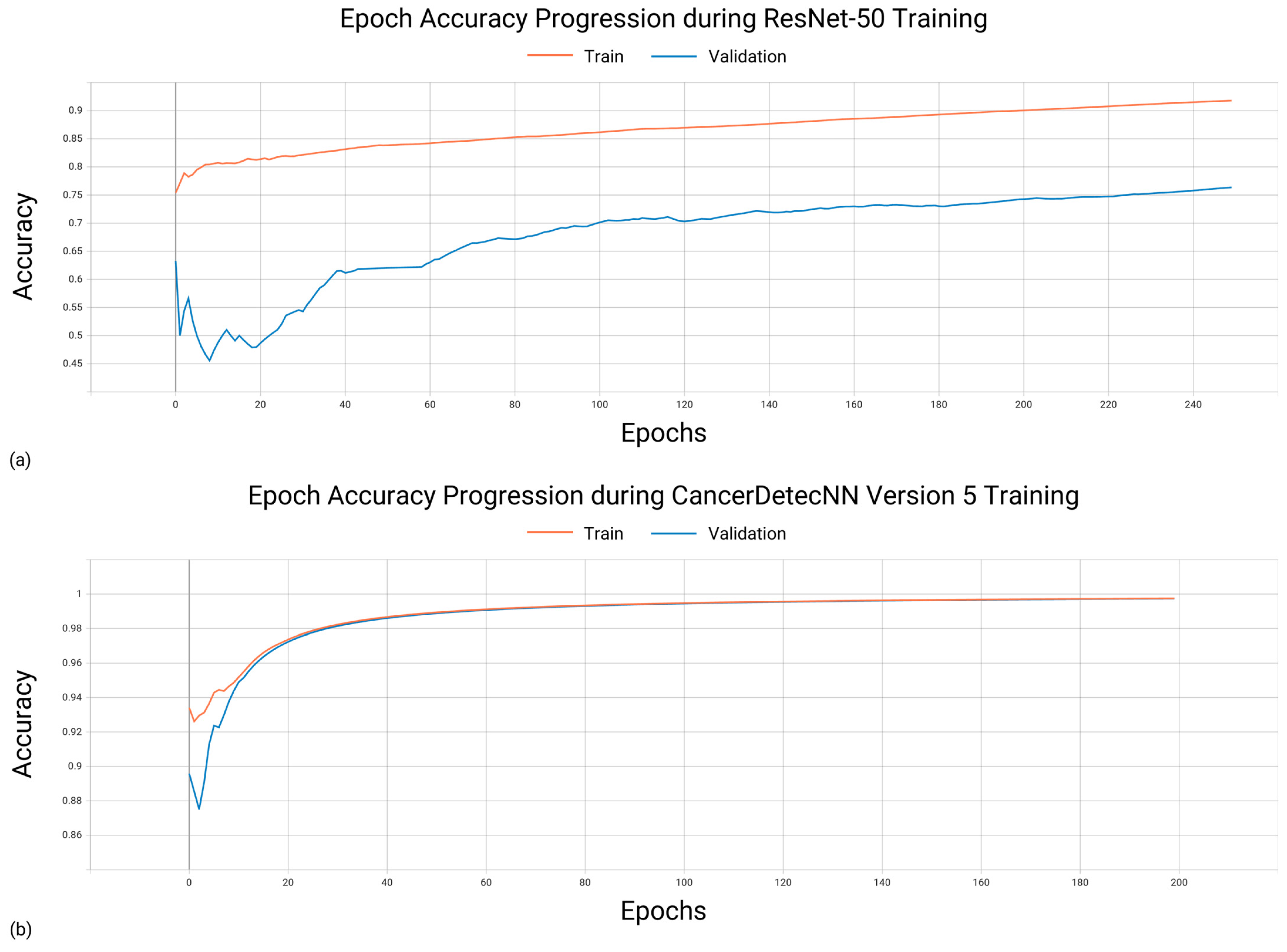
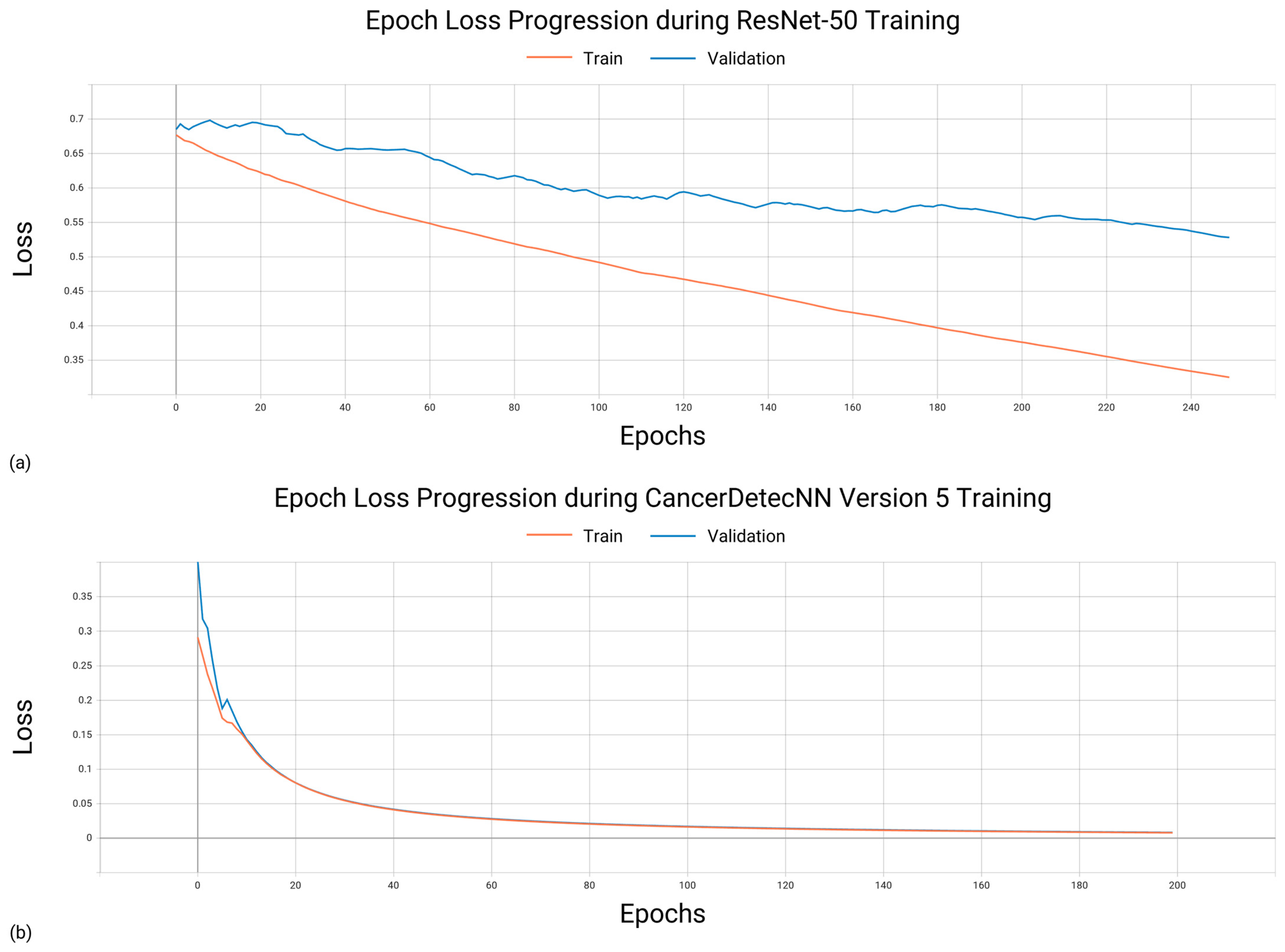
3.1. Training Characteristics
3.2. Hardware and Software Configuration
- Central Process Unit(s): 2 × CPU AMD EPYC ROME 7452 32C/64T 2.35 GHZ 128 MB SP3 155 W;
- Random Access Memory: 16 × DIMM HYNIX 32 GB DDR4 3200 MHZ NR ECCR;
- Graphical Process Unit(s): 4 × NVIDIA TESLA A100 40 GB;
- Physical Memory: 2 × SSD WESTERN DIGITAL DC SN640 3.84 TB NVME PCI-E 2.5″ 0.8 DWPD.
3.3. Evaluating the Performance of Existing Convolutional Neural Networks
Comparing Training Time of Existing CNNs for Optimal Performance
3.4. Evaluating the Performance of CancerDetecNN
Comparing Training Time of CancerDetecNNs for Optimal Performance
3.5. Comparative Analysis of the Convolutional Neural Networks
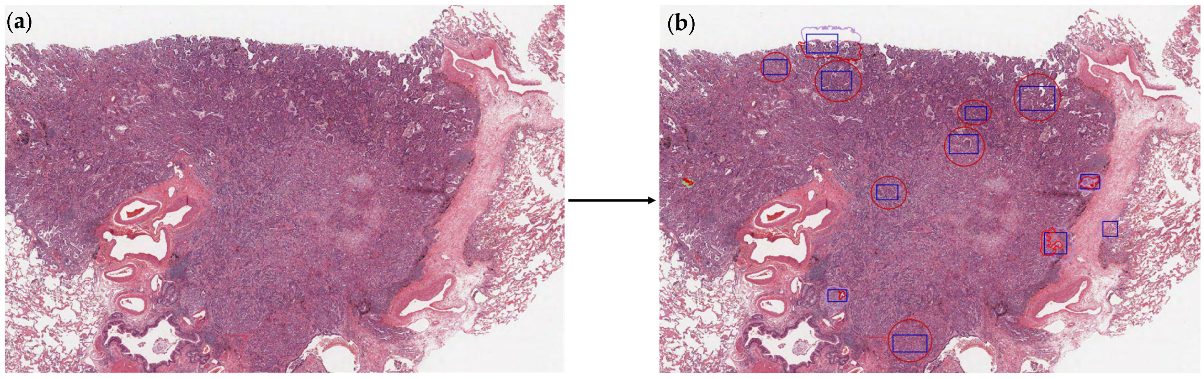
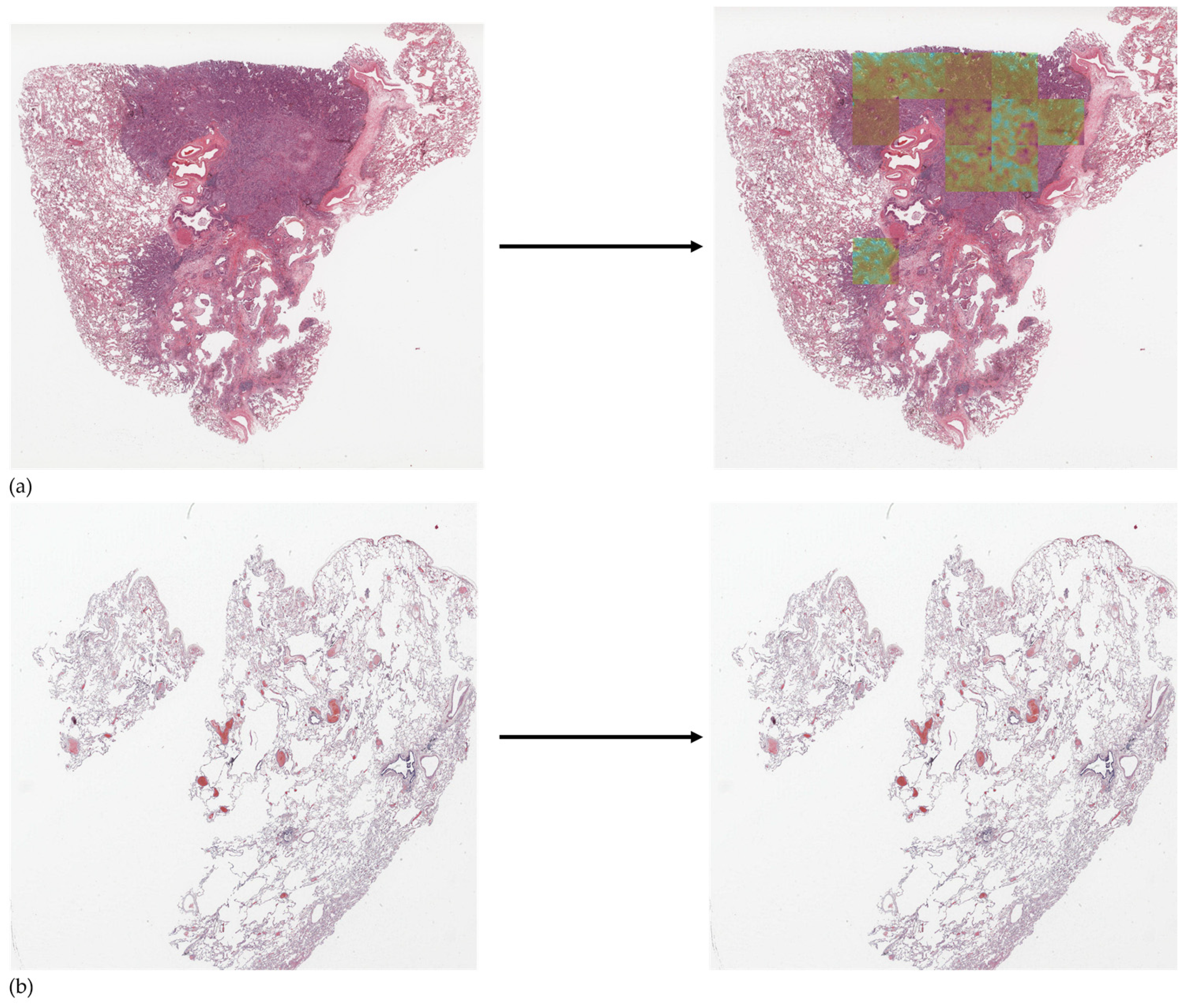
3.6. Detection Using CancerDetecNN Version 5
4. Conclusions and Future Work
Author Contributions
Funding
Institutional Review Board Statement
Informed Consent Statement
Data Availability Statement
Acknowledgments
Conflicts of Interest
Appendix A


References
- World Health Organization Cancer. Available online: https://www.who.int/news-room/fact-sheets/detail/cancer (accessed on 24 February 2023).
- Nasim, F.; Sabath, B.F.; Eapen, G.A. Lung Cancer. Med. Clin. N. Am. 2019, 103, 463–473. [Google Scholar] [CrossRef] [PubMed]
- Faria, N.; Campelos, S.; Carvalho, V. Cancer Detec—Lung Cancer Diagnosis Support System: First Insights. In Proceedings of the 15th International Joint Conference on Biomedical Engineering Systems and Technologies—Volume 3: BIOINFORMATICS, Online, 9–11 February 2022; pp. 83–90, ISBN 978-989-758-552-4. [Google Scholar]
- Bade, B.C.; dela Cruz, C.S. Lung Cancer 2020: Epidemiology, Etiology, and Prevention. Clin. Chest Med. 2020, 41, 1–24. [Google Scholar] [CrossRef] [PubMed]
- Duma, N.; Santana-Davila, R.; Molina, J.R. Non–Small Cell Lung Cancer: Epidemiology, Screening, Diagnosis, and Treatment. Mayo Clin. Proc. 2019, 94, 1623–1640. [Google Scholar] [CrossRef] [PubMed]
- Polanski, J.; Jankowska-Polanska, B.; Rosinczuk, J.; Chabowski, M.; Szymanska-Chabowska, A. Quality of Life of Patients with Lung Cancer. Onco Targets Ther. 2016, 9, 1023–1028. [Google Scholar] [CrossRef] [PubMed]
- Travis, W.D.; Brambilla, E.; Nicholson, A.G.; Yatabe, Y.; Austin, J.H.M.; Beasley, M.B.; Chirieac, L.R.; Dacic, S.; Duhig, E.; Flieder, D.B.; et al. The 2015 World Health Organization Classification of Lung Tumors: Impact of Genetic, Clinical and Radiologic Advances Since the 2004 Classification. J. Thorac. Oncol. 2015, 10, 1243–1260. [Google Scholar] [CrossRef]
- Bera, K.; Schalper, K.A.; Rimm, D.L.; Velcheti, V.; Madabhushi, A. Artificial Intelligence in Digital Pathology — New Tools for Diagnosis and Precision Oncology. Nat. Rev. Clin. Oncol. 2019, 16, 703. [Google Scholar] [CrossRef]
- Faria, N.; Campelos, S.; Carvalho, V. Development of a Lung Cancer Diagnosis Support System; IARIA: Porto, Portugal, 2022; pp. 30–32. [Google Scholar]
- De Koning, H.J.; van der Aalst, C.M.; de Jong, P.A.; Scholten, E.T.; Nackaerts, K.; Heuvelmans, M.A.; Lammers, J.-W.J.; Weenink, C.; Yousaf-Khan, U.; Horeweg, N.; et al. Reduced Lung-Cancer Mortality with Volume CT Screening in a Randomized Trial. New. Engl. J. Med. 2020, 382, 503–513. [Google Scholar] [CrossRef]
- Howlader, N.; Forjaz, G.; Mooradian, M.J.; Meza, R.; Kong, C.Y.; Cronin, K.A.; Mariotto, A.B.; Lowy, D.R.; Feuer, E.J. The Effect of Advances in Lung-Cancer Treatment on Population Mortality. N. Engl. J. Med. 2020, 383, 640. [Google Scholar] [CrossRef]
- Knight, S.B.; Crosbie, P.A.; Balata, H.; Chudziak, J.; Hussell, T.; Dive, C. Progress and Prospects of Early Detection in Lung Cancer. Open. Biol. 2017, 7, 170070. [Google Scholar] [CrossRef]
- Bi, W.L.; Hosny, A.; Schabath, M.B.; Giger, M.L.; Birkbak, N.J.; Mehrtash, A.; Allison, T.; Arnaout, O.; Abbosh, C.; Dunn, I.F.; et al. Artificial Intelligence in Cancer Imaging: Clinical Challenges and Applications. CA Cancer J. Clin. 2019, 69, 127–157. [Google Scholar] [CrossRef]
- Gour, M.; Jain, S.; Sunil Kumar, T. Residual Learning Based CNN for Breast Cancer Histopathological Image Classification. Int. J. Imaging Syst. Technol. 2020, 30, 621–635. [Google Scholar] [CrossRef]
- Garg, R.; Maheshwari, S.; Shukla, A. Decision Support System for Detection and Classification of Skin Cancer Using CNN. Adv. Intell. Syst. Comput. 2021, 1189, 578–586. [Google Scholar] [CrossRef]
- Ezhilarasi, R.; Varalakshmi, P. Tumor Detection in the Brain Using Faster R-CNN. In Proceedings of the 2018 2nd International Conference on I-SMAC (IoT in Social, Mobile, Analytics and Cloud) (I-SMAC)I-SMAC (IoT in Social, Mobile, Analytics and Cloud) (I-SMAC), Palladam, India, 30–31 August 2018; pp. 388–392. [Google Scholar] [CrossRef]
- Litjens, G.; Kooi, T.; Bejnordi, B.E.; Setio, A.A.A.; Ciompi, F.; Ghafoorian, M.; van der Laak, J.A.W.M.; van Ginneken, B.; Sánchez, C.I. A Survey on Deep Learning in Medical Image Analysis. Med. Image Anal. 2017, 42, 60–88. [Google Scholar] [CrossRef] [PubMed]
- Yamashita, R.; Nishio, M.; Do, R.K.G.; Togashi, K. Convolutional Neural Networks: An Overview and Application in Radiology. Insights Imaging 2018, 9, 611–629. [Google Scholar] [CrossRef] [PubMed]
- Ardila, D.; Kiraly, A.P.; Bharadwaj, S.; Choi, B.; Reicher, J.J.; Peng, L.; Tse, D.; Etemadi, M.; Ye, W.; Corrado, G.; et al. End-to-End Lung Cancer Screening with Three-Dimensional Deep Learning on Low-Dose Chest Computed Tomography. Nat. Med. 2019, 25, 954–961. [Google Scholar] [CrossRef] [PubMed]
- Wang, S.; Chen, A.; Yang, L.; Cai, L.; Xie, Y.; Fujimoto, J.; Gazdar, A.; Xiao, G. Comprehensive Analysis of Lung Cancer Pathology Images to Discover Tumor Shape and Boundary Features That Predict Survival Outcome. Sci. Rep. 2018, 8, 10393. [Google Scholar] [CrossRef]
- Coudray, N.; Ocampo, P.S.; Sakellaropoulos, T.; Narula, N.; Snuderl, M.; Fenyö, D.; Moreira, A.L.; Razavian, N.; Tsirigos, A. Classification and Mutation Prediction from Non–Small Cell Lung Cancer Histopathology Images Using Deep Learning. Nat. Med. 2018, 24, 1559–1567. [Google Scholar] [CrossRef]
- Burlutskiy, N.; Gu, F.; Wilen, L.K.; Backman, M.; Micke, P. A Deep Learning Framework for Automatic Diagnosis in Lung Cancer. arXiv 2018, arXiv:1807.10466. [Google Scholar]
- Li, Z.; Hu, Z.; Xu, J.; Tan, T.; Chen, H.; Duan, Z.; Liu, P.; Tang, J.; Cai, G.; Ouyang, Q.; et al. Computer-Aided Diagnosis of Lung Carcinoma Using Deep Learning—A Pilot Study. arXiv 2018, arXiv:1803.05471. [Google Scholar]
- Yu, K.H.; Wang, F.; Berry, G.J.; Ré, C.; Altman, R.B.; Snyder, M.; Kohane, I.S. Classifying Non-Small Cell Lung Cancer Types and Transcriptomic Subtypes Using Convolutional Neural Networks. J. Am. Med. Inform. Assoc. 2020, 27, 757–769. [Google Scholar] [CrossRef]
- Saric, M.; Russo, M.; Stella, M.; Sikora, M. CNN-Based Method for Lung Cancer Detection in Whole Slide Histopathology Images. In Proceedings of the 2019 4th International Conference on Smart and Sustainable Technologies (SpliTech), Split, Croatia, 18–21 June 2019. [Google Scholar] [CrossRef]
- Hatuwal, B.K.; Chand Thapa, H. Lung Cancer Detection Using Convolutional Neural Network on Histopathological Images. Artic. Int. J. Comput. Trends Technol. 2020, 68, 21–24. [Google Scholar] [CrossRef]
- Chen, C.L.; Chen, C.C.; Yu, W.H.; Chen, S.H.; Chang, Y.C.; Hsu, T.I.; Hsiao, M.; Yeh, C.Y.; Chen, C.Y. An Annotation-Free Whole-Slide Training Approach to Pathological Classification of Lung Cancer Types Using Deep Learning. Nat. Commun. 2021, 12, 1193. [Google Scholar] [CrossRef] [PubMed]
- Jehangir, B.; Nayak, S.R.; Shandilya, S. Lung Cancer Detection Using Ensemble of Machine Learning Models. In Proceedings of the Confluence 2022—12th International Conference on Cloud Computing, Data Science and Engineering, Noida, India, 27–28 January 2022; pp. 411–415. [Google Scholar] [CrossRef]
- Wahid, R.R.; Nisa, C.; Amaliyah, R.P.; Puspaningrum, E.Y. Lung and Colon Cancer Detection with Convolutional Neural Networks on Histopathological Images. AIP Conf. Proc. 2023, 2654, 020020. [Google Scholar] [CrossRef]
- National Cancer Institute. NLST—The Cancer Data Access System. Available online: https://cdas.cancer.gov/nlst/ (accessed on 24 February 2023).
- National Cancer Institute. The Cancer Genome Atlas Program (TCGA). Available online: https://www.cancer.gov/ccg/research/genome-sequencing/tcga (accessed on 24 February 2023).
- Krizhevsky, A.; Sutskever, I.; Hinton, G.E. ImageNet Classification with Deep Convolutional Neural Networks. Adv. Neural Inf. Process. Syst. 2012, 25. [Google Scholar] [CrossRef]
- Szegedy, C.; Liu, W.; Jia, Y.; Sermanet, P.; Reed, S.; Anguelov, D.; Erhan, D.; Vanhoucke, V.; Rabinovich, A. Going Deeper with Convolutions. In Proceedings of the IEEE Computer Society Conference on Computer Vision and Pattern Recognition, Boston, MA, USA, 1–12 June 2015; pp. 1–9. [Google Scholar]
- He, K.; Zhang, X.; Ren, S.; Sun, J. Deep Residual Learning for Image Recognition. In Proceedings of the IEEE Computer Society Conference on Computer Vision and Pattern Recognition, Las Vegas, NV, USA, 27–30 June 2016; pp. 770–778. [Google Scholar]
- Pan, S.J.; Yang, Q. A Survey on Transfer Learning. IEEE Trans. Knowl. Data Eng. 2010, 22, 1345–1359. [Google Scholar] [CrossRef]
- Müller, D.; Soto-Rey, I.; Kramer, F. Towards a Guideline for Evaluation Metrics in Medical Image Segmentation. BMC Res. Notes 2022, 15, 210. [Google Scholar] [CrossRef]
- Roberto, G.F.; Lumini, A.; Neves, L.A.; do Nascimento, M.Z. Fractal Neural Network: A New Ensemble of Fractal Geometry and Convolutional Neural Networks for the Classification of Histology Images. Expert. Syst. Appl. 2021, 166, 114103. [Google Scholar] [CrossRef]


| Authors | Methods | Datasets | Results |
|---|---|---|---|
| Wang et al. (2018) [20] | CNN based on inception V3 algorithm using sliding grid mechanism | 267 training and 457 validation ADC WSIs | Accuracy of 0.898 |
| Coudray et al. (2018) [21] | CNN based on inception V3 algorithm using tiles sizes of 512 × 512 pixels | 1635 slides (ADC, non-malignant, SCC) | Average AUC of 0.97. |
| Nikolay et al. (2018) [22] | Seven different architectures including UNet | 712 annotated WSIs | Precision of 0.80, F1-score of 0.80, recall of 0.86. |
| Li et al. (2018) [23] | AlexNet, VGG, ResNet, and SqueezeNet CNNs | 33 lung patients | AUC results for training from scratch: 0.912 (AlexNet), 0.911 (SqueezeNet), 0.891 (ResNet), 0.881 (VGGNet). AUC results for fine tuning: 0.859 (AlexNet), 0.875 (SqueezeNet), 0.869 (ResNet), 0.830 (VGGNet). |
| Yu et al. (2019) [24] | Pre-trained CNNs (AlexNet, VGG-16, GoogLeNet, and ResNet-50) using tiles of 1000 × 1000 pixels | 1314 ADC and SCC WSIs | AUC values detecting ADC: 0.890 for AlexNet, 0.912 for VGG-16, 0.901 for GoogLeNet, and 0.935 for ResNet-50. AUC values detecting SCC: 0.995 for AlexNet, 0.991 for VGG-16, 0.993 for GoogLeNet, and 0.979 for ResNet-50. |
| Sarić et al. (2019) [25] | CNNs VGG-16 and ResNet-50 using patches of 256 × 256 pixels | 25 lung WSIs | ROC values of 0.833 (VGG-16) and 0.796 (ResNet-50). |
| Hatuwal and Thapa (2020) [26] | Custom CNN with tiles resized to 180 × 180 pixels | 5000 histopathology images per category (benign, ADC, SCC) | Precision of 0.95, recall of 0.97, F1-score of 0.96 (ADC); precision of 1.00, recall of 1.00, F1-score of 1.00 (benign); precision of 0.97, recall of 0.95, F1-score of 0.96 (SCC). |
| Chen et al. (2021) [27] | ResNet-50 using original WSI as input | 9662 lung cancer WSIs | AUC of 0.9594 (ADC) and 0.9414 (SCC). |
| Jehangir et al. (2022) [28] | Custom CNN | 5000 histopathology images per category (benign, ADC, SCC) | Precision of 0.933, recall of 0.717, F1-score of 0.811 (ADC); precision of 1.00, recall of 0.943, F1-score of 0.971 (benign); precision of 0.774, recall of 0.998, F1-score of 0.872 (SCC); |
| Wahid et al. (2023) [29] | Pre-trained CNNs (GoogLeNet, ResNet-18, and SuffleNet V2) and custom CNN | 5000 histopathology images per category (benign, ADC, SCC) | GoogLeNet F1-scores: 0.96 for ADC, 1.00 for benign, 0.97 for SCC. ResNet-18 F1-scores: 0.98 for ADC, 1.00 for benign, 0.98 for SCC. ShuffleNet V2 F1-scores: 0.96 for ADC, 1.00 for benign, 0.96 for SCC. Custom CNN F1-scores: 0.89 for ADC, 0.98 for benign, 0.91 for SCC. |
| Repository | Number of Cases | Number of WSIs |
|---|---|---|
| NLST [30] | 449 | 1221 |
| TCGA [31] | 582 | 821 |
| Transformation | Parameters |
|---|---|
| Rescaling | 1/255 |
| Shearing | Intensity = 0.2 |
| Rotation | Angle up to 0.2 radians |
| Zoom | Range of 0.5 |
| Flip | Horizontal |
| CNN | Number of Parameters |
|---|---|
| AlexNet | 46,756,609 |
| GoogLeNet | 8,471,347 |
| ResNet-50 | 25,637,713 |
| CancerDetecNN V0 | 929 |
| CancerDetecNN V1 | 18,305 |
| CancerDetecNN V3 | 53,185 |
| CancerDetecNN V4 | 159,809 |
| CancerDetecNN V5 | 307,393 |
| CancerDetecNN V6 | 520,513 |
| CancerDetecNN V7 | 520,513 |
| CancerDetecNN V8 | 700,097 |
| CancerDetecNN V9 | 776,801 |
| CancerDetecNN V10 | 793,121 |
| CancerDetecNN V11 | 454,977 |
| CancerDetecNN V12 | 240,961 |
| Characteristic | Value |
|---|---|
| k-fold cross-validation | 10 |
| Dataset Ratio | 80:20 |
| Epochs | 50, 100, 150, 200, 250, 300 |
| Optimizer | Adam |
| Loss Function | Binary Cross-entropy |
| Epochs | CNN | Accuracy | Precision | Recall | AUC | F1-Score |
|---|---|---|---|---|---|---|
| 50 | AlexNet | 0.688 | 0.742 | 0.848 | 0.723 | 0.792 |
| GoogLeNet | 0.817 | 0.868 | 0.821 | 0.836 | 0.843 | |
| ResNet-50 | 0.739 | 0.848 | 0.745 | 0.755 | 0.793 | |
| ResNet-50 Pre-trained | 0.767 | 0.821 | 0.852 | 0.810 | 0.836 | |
| 100 | AlexNet | 0.707 | 0.866 | 0.670 | 0.738 | 0.755 |
| GoogLeNet | 0.826 | 0.867 | 0.840 | 0.845 | 0.853 | |
| ResNet-50 | 0.806 | 0.852 | 0.834 | 0.828 | 0.843 | |
| ResNet-50 Pre-trained | 0.811 | 0.865 | 0.818 | 0.843 | 0.841 | |
| 150 | AlexNet | 0.821 | 0.885 | 0.815 | 0.836 | 0.849 |
| GoogLeNet | 0.758 | 0.778 | 0.711 | 0.791 | 0.743 | |
| ResNet-50 | 0.785 | 0.887 | 0.753 | 0.835 | 0.815 | |
| ResNet-50 Pre-trained | 0.815 | 0.854 | 0.859 | 0.825 | 0.857 | |
| 200 | AlexNet | 0.749 | 0.853 | 0.736 | 0.778 | 0.790 |
| GoogLeNet | 0.823 | 0.861 | 0.841 | 0.841 | 0.851 | |
| ResNet-50 | 0.813 | 0.830 | 0.747 | 0.853 | 0.828 | |
| ResNet-50 Pre-trained | 0.807 | 0.910 | 0.767 | 0.843 | 0.833 | |
| 250 | AlexNet | 0.752 | 0.841 | 0.793 | 0.760 | 0.816 |
| GoogLeNet | 0.811 | 0.869 | 0.805 | 0.831 | 0.836 | |
| ResNet-50 | 0.839 | 0.894 | 0.836 | 0.856 | 0.864 | |
| ResNet-50 Pre-trained | 0.777 | 0.864 | 0.781 | 0.791 | 0.820 | |
| 300 | AlexNet | 0.814 | 0.873 | 0.818 | 0.826 | 0.845 |
| GoogLeNet | 0.802 | 0.855 | 0.818 | 0.837 | 0.836 | |
| ResNet-50 | 0.798 | 0.805 | 0.756 | 0.821 | 0.780 | |
| ResNet-50 Pre-trained | 0.816 | 0.929 | 0.753 | 0.860 | 0.832 |
| Epochs | CNN | Accuracy | Precision | Recall | AUC | F1-Score | Training Time |
|---|---|---|---|---|---|---|---|
| 150 | AlexNet | 0.821 | 0.885 | 0.815 | 0.836 | 0.849 | 2 h 22 min |
| ResNet-50 Pre-trained | 0.815 | 0.854 | 0.859 | 0.825 | 0.857 | 2 h 37 min | |
| 200 | GoogLeNet | 0.823 | 0.861 | 0.841 | 0.841 | 0.851 | 2 h 07 min |
| 250 | ResNet-50 | 0.839 | 0.894 | 0.836 | 0.856 | 0.864 | 3 h 23 min |
| Epochs | CancerDetecNN Version | Accuracy | Precision | Recall | AUC | F1-Score |
|---|---|---|---|---|---|---|
| 50 | 5 | 0.861 | 0.960 | 0.803 | 0.927 | 0.874 |
| 6 | 0.839 | 0.918 | 0.805 | 0.901 | 0.858 | |
| 7 | 0.849 | 0.983 | 0.762 | 0.920 | 0.858 | |
| 12 | 0.836 | 0.942 | 0.779 | 0.911 | 0.853 | |
| 100 | 5 | 0.834 | 0.884 | 0.837 | 0.893 | 0.860 |
| 6 | 0.872 | 0.957 | 0.823 | 0.926 | 0.885 | |
| 7 | 0.872 | 0.968 | 0.814 | 0.930 | 0.884 | |
| 12 | 0.761 | 0.962 | 0.626 | 0.860 | 0.758 | |
| 150 | 5 | 0.833 | 0.972 | 0.833 | 0.895 | 0.847 |
| 6 | 0.860 | 0.935 | 0.827 | 0.915 | 0.878 | |
| 7 | 0.866 | 0.946 | 0.827 | 0.905 | 0.883 | |
| 12 | 0.841 | 0.916 | 0.816 | 0.894 | 0.863 | |
| 200 | 5 | 0.885 | 0.972 | 0.833 | 0.923 | 0.897 |
| 6 | 0.836 | 0.921 | 0.800 | 0.895 | 0.856 | |
| 7 | 0.861 | 0.925 | 0.836 | 0.890 | 0.878 | |
| 12 | 0.820 | 0.946 | 0.752 | 0.882 | 0.838 | |
| 250 | 5 | 0.839 | 0.956 | 0.767 | 0.892 | 0.851 |
| 6 | 0.866 | 0.979 | 0.795 | 0.910 | 0.877 | |
| 7 | 0.841 | 0.871 | 0.863 | 0.878 | 0.867 | |
| 12 | 0.766 | 0.919 | 0.666 | 0.830 | 0.772 | |
| 300 | 5 | 0.841 | 0.935 | 0.789 | 0.880 | 0.856 |
| 6 | 0.881 | 0.936 | 0.860 | 0.909 | 0.897 | |
| 7 | 0.842 | 0.900 | 0.836 | 0.890 | 0.867 | |
| 12 | 0.871 | 0.955 | 0.825 | 0.909 | 0.885 |
| Epochs | CancerDetecNN Version | Accuracy | Precision | Recall | AUC | F1-Score | Training Time |
|---|---|---|---|---|---|---|---|
| 100 | 7 | 0.872 | 0.968 | 0.814 | 0.930 | 0.884 | 1 h 20 min |
| 200 | 5 | 0.885 | 0.972 | 0.833 | 0.923 | 0.897 | 1 h 32 min |
| 300 | 6 | 0.881 | 0.936 | 0.860 | 0.909 | 0.897 | 1 h 40 min |
| 12 | 0.871 | 0.955 | 0.825 | 0.909 | 0.885 | 1 h 41 min |
| Actual Positive | Actual Negative | |
|---|---|---|
| Predicted Positive | 60.8 | 1.8 |
| Predicted Negative | 12.2 | 47.2 |
Disclaimer/Publisher’s Note: The statements, opinions and data contained in all publications are solely those of the individual author(s) and contributor(s) and not of MDPI and/or the editor(s). MDPI and/or the editor(s) disclaim responsibility for any injury to people or property resulting from any ideas, methods, instructions or products referred to in the content. |
© 2023 by the authors. Licensee MDPI, Basel, Switzerland. This article is an open access article distributed under the terms and conditions of the Creative Commons Attribution (CC BY) license (https://creativecommons.org/licenses/by/4.0/).
Share and Cite
Faria, N.; Campelos, S.; Carvalho, V. A Novel Convolutional Neural Network Algorithm for Histopathological Lung Cancer Detection. Appl. Sci. 2023, 13, 6571. https://doi.org/10.3390/app13116571
Faria N, Campelos S, Carvalho V. A Novel Convolutional Neural Network Algorithm for Histopathological Lung Cancer Detection. Applied Sciences. 2023; 13(11):6571. https://doi.org/10.3390/app13116571
Chicago/Turabian StyleFaria, Nelson, Sofia Campelos, and Vítor Carvalho. 2023. "A Novel Convolutional Neural Network Algorithm for Histopathological Lung Cancer Detection" Applied Sciences 13, no. 11: 6571. https://doi.org/10.3390/app13116571
APA StyleFaria, N., Campelos, S., & Carvalho, V. (2023). A Novel Convolutional Neural Network Algorithm for Histopathological Lung Cancer Detection. Applied Sciences, 13(11), 6571. https://doi.org/10.3390/app13116571