A Labelling Method for the Travelling Salesman Problem

Abstract

The travelling salesman problem (TSP) is a problem whereby a finite number of nodes are supposed to be visited exactly once, one after the other, in such a way that the total weight of connecting arcs used to visit these nodes is minimized. We propose a labelling method to solve the TSP problem. The algorithm terminates after K−1 iterations, where K is the total number of nodes in the network. The algorithm’s design allows it to determine alternative tours if there are any in the TSP network. The computational complexity of the algorithm reduces as iterations increase, thereby making it a powerful and efficient algorithm. Numerical illustrations are used to prove the efficiency and validity of the proposed algorithm.

1. Introduction

The travelling salesman is defined as a network $G$, given by $G=\left(K,L\right)$, where $K$ denotes the set of nodes in the network and $L$ denotes the set of links in the network. For convenience, node 1 is considered as the home city. Starting from node 1, the salesman has to visit $K-1$ nodes exactly once and return to the home city while minimizing the travelled distance. The nodes in the network may represent locations, cites, game parks, mountains, airports and countries, among others. Network arcs represent roads, railway lines and rivers, among others. The TSP can be classified as a symmetric TSP or non-symmetric TSP. The TSP is a combinatorial optimization problem that is very complex to solve since it changes to form new variants as technology improves. The cost-constrained travelling salesman problem (CCTSP) in Sokkappa [1], price collecting travelling salesman problem (PCTSP) in Dogan and Alkaya [2], maximum scatter travelling salesman problem (MSTSP) in Venkatesh et al. [3], vehicle routing problem (VRP) in Vincent et al. [4], equality generalized travelling salesman problem E-GTSP in Tawanda et al. [5] and clustered travelling salesman problem (CTSP) in Kawasaki and Takazawa [6] are some of the variants of TSP. Many algorithms and heuristics such as the Greedy Algorithm (GA), Dynamic Programming (DP), Simulated annealing algorithm (SA), Neighborhood search algorithm (NSA), Genetic Algorithm (GA) and TABU Search algorithm (TA) are among the well-known developed algorithms used to solve the TSP.

Motivation

The travelling salesman problem is a combinatorial optimization problem that is very difficult to solve and has many applications in life. The TSP has been branching to form new variants as technology improves. The TSP and its variants have proved to be very difficult to solve; this is evidenced by many algorithms that have been proposed in the past decades. As a result, there is a need to keep on developing, modifying and combining existing algorithms to form hybrid algorithms. Many algorithms such as the GA depend on computer codes to solve the TSP and require many iterations to compute optimal or near optimal tours. There is a need to develop algorithms that are able to compute alternative optimal tours if the network has one. The need to develop algorithms which are not only computer-code-dependent for solving the TSP has motivated this research, as well as the need to develop simple and efficient algorithms that can be used for teaching purposes and solving the TSP and its variants.

2. Literature Review

The travelling salesman problem (TSP) through the K set of nodes was considered by Srivastava et al. [7] and Garg et al. [8]. Kumar et al. [9] developed a TSP heuristic that is based on the Minimum spanning tree (MST). Kumar et al. [10] established a relationship between the MST under the index restriction and the Minimum travelling salesman tour (MTST). The MST-based heuristic approach reduces TSP complexity; however, the worst case arises in the case of a completely connected network. Munapo [11] proposed a Branch and bound (BB) approach, where TSP is broken into sub-problems that are then solved as MST models. The research revealed that the MST-based approach is efficient in solving the TSP. Munapo [12] presented a network reconstruction approach for solving the TSP. In this approach, TSP sub-tours are detected by MST, and sub-tours are then eliminated through the TSP network reconstruction using dummy nodes as bridges. Saksena and Kumar [13] considered a K-specified nodes routing problem. The problem converges to the TSP problem when K = N−1, where N is the number of nodes in a given network. Munapo et al. [14] proposed a minimum weight label method for determining the longest and shortest paths in directed graphs; this approach was applied to project networks as an alternative to Critical path method (CPM). Kumar et al. [15] developed a minimum weight labelling method for finding the shortest path. For a K-node network, the algorithm computes the shortest path in K−1 iterations. Tawanda [16] developed a non-iterative algorithm for determining the shortest path, and the algorithm transforms a network to a tree through arc and node replications. Maposa et al. [17] proposed a non-iterative shortest path algorithm; the algorithm makes use of a $n\times n$ tableau to compute the shortest path. The algorithm computes the shortest path within a reasonable time as compared to other iterative techniques. Akhand et al. [18] proposed the Discrete Spider Monkey Optimization (SMO). The algorithm is based on the social behavior of monkeys. The efficiency of the SMO was demonstrated using large TSP instances as well as a comparison analysis with other TSP algorithms such as Ant Colony Optimization (ACO), among others. Panwar and Deep [19] presented the discrete Grey Wolf Optimizer D-(GWO) that is inspired by the behavior of grey wolves. A 2-Opt procedure was used in combination with D-(GWO) to improve the solution. Computational experiments proved that D-(GWO) outperforms Bat Algorithm and the Imperialist competitive algorithm. Gharehchopogh and Abdollahzadeh [20] solved the TSP using the Harris hawk optimization (HHO) algorithm. The Lin and Kerninghan heuristic (LKH), local search strategy and Metropolis acceptance strategy were also used to improve the performance of the algorithm. The algorithm was proved to be efficient based on 80 TSP instances from the TSP LIBRARY (TSPLIB). Taillard and Helsgaun [21] solved the TSP using The partial optimization metaheuristic under special intensification conditions (POPMUSIC). The POPMUSIC metaheuristic was tested on several TSP instances and it was proved to be efficient; however, there is a need to work on reducing the algorithm time complexity. Eremeev and Kovalenko [22] developed a memetic algorithm that uses 3-Opt local search to improve the solution. The algorithm yields competitive results when compared to other state-of-the-art algorithms. Arigliano et al. [23] developed a branch and bound algorithm that is capable of solving the time-dependent TSP with up to 50 vertices. The algorithm computes a better solution when compared to the Branch and Cut procedure. Hatamlou [24] solved the TSP using the Black hole (BH) algorithm. The BH algorithm is inspired by the black hole phenomenon and is population-based. Computational results have demonstrated that the BH algorithm outperforms ACO, Genetic algorithm (GA) and Particle swarm optimization (PSO). Gao [25] improved the ACO algorithm by combining searching ants. Based on eight TSP instances, they solved the new method and outperformed the traditional ACO algorithm in terms of the solution accuracy and computational effort required. Dahan et al. [26] presented a Dynamic flying ant colony optimization (DFACO). DFACO is a modification of ACO; the modifications include the use of a 3-Opt local search to help the algorithm escape local minima. Computational results demonstrate that the DFACO performs better than ACO. Boccia et al. [27] proposed a new method to solve the TSP by combining the Column and row method and the Branch and Cut algorithm. The algorithm managed to compute good solutions on TSP problems with 10–20 cities. Gunduz and Aslan [28] modified the JAYA algorithm to the Discrete JAYA algorithm (DJAYA). The DJAYA algorithm generates initial solutions using random permutations and the nearest neighborhood approach. A 2-Opt local search is used to improve the best solution found by the DJAYA algorithm. The DJAYA algorithm performs better than the ACO and Black hole (BH) algorithm. Zhan et al. [29] presented a List-based simulated annealing (LBSA) algorithm. The algorithm creates a list of temperatures; the maximum temperature in the list is used to accept or reject a solution candidate. Computational comparisons revealed that the LBSA algorithm is capable of computing good solutions. Akhand et al. [30] developed a Producer–Scrounger method (PSM) for TSP. The method is inspired by the behavior of a group of animals. Computational experiments proved that PSM outperformed the GA and ACO. Hussain et al. [31] introduced the genetic algorithm with a modified cycle crossover operator (CX2) to solve the TSP. Computational comparisons revealed that the CX2 computed better TSP solutions than operators such as the partially mapped crossover (PMX) and ordered crossover (OX). Al-Dallal [32] proposed two genetic algorithm operators, the two-point crossover with replacement (TPXwR) and Combinatorial crossover technique (CXT). TPXwR and CXT operators were compared with the OX operator; the results revealed that the CXT outperformed both OX and TPXwR.

3. Mathematical Model for TSP

Define the following variables:

$$x_{ij}=\{\begin{array}{l}1, if node i is connected to node j \\ 0, Otherwise \end{array}$$

$$\Vert c_{ij}\Vert -cost matrix$$

$$k-number of nodes$$

The general TSP model is given as follows:

$$Minimise Z={\displaystyle \sum }_{i=1}^k{\displaystyle \sum }_{j=1}^k{c}_{ij}{x}_{ij}, c_{ij}=\infty for all i=j$$

Subjected to

$${\displaystyle \sum }_{j=1}^k{x}_{ij}=1, for i=1, 2, \dots , k$$

$${\displaystyle \sum }_{i=1}^k{x}_{ij}=1, for j=1, 2, \dots , k$$

$$x_{ij}=\left(0,1\right)$$

When $c_{ij}=c_{ji} \forall i and j$, the TSP is said to be a symmetrical TSP; otherwise, it is said to be an asymmetrical TSP. There are several ways of formulating the mathematical model for the TSP. See Munapo [11] and Taha [33].

4. Method of Solution: Labelling Method

Munapo et al. [14] introduced a labelling method to compute a critical path in project networks. The same labelling method was modified by Kumar et al. [15] to develop a shortest path algorithm for non-directed networks. In this paper, we modify the labelling method and develop a new labelling method to solve the TSP.

4.1. Definition of Terms

The following definitions are associated with the development of the algorithm.

4.1.1. Definition 1: Sets of Nodes

$L_0$ = The set of intermediate nodes, and it is given by $L_0=\left\{2,3,\dots ,k\right\}$. This set is said to be empty, thus $L_0=\{\varnothing \}$ when all the elements are included in all partial tour(s). The elements of this set must be included exactly once in each and every tour. $L^{*}{}_0$ = the set that contains the source and destination node of the travelling salesman network, thus $L^{*}{}_0=\left\{1\right\}.$ The element of this set should be at the extremes of each and every valid tour.

4.1.2. Definition 2: Node Label

Given a network with node 1 as the home city and other intermediate nodes as {2, 3, 4, …, n}, a generalized node label is given by $w_{{\left(1,j\right)}^z}$, where $j$ is the currently added node to the partial tour $\left(1,j\right)$ with z intermediate nodes. W is the total weight or cost of travelling from node 1 to the currently added node $j$ through $z$ intermediate nodes. Another label $(\infty )$ is used to restrict adding node $k$ to the node label if node $k$ is already part of the node label.

4.1.3. Definition 3: Minimum Weight Label

For every node $=j$, $k\in L_0$, the minimum weight label, is given by $w^{*}{}_{{\left(1,k\right)}^z}=\mathrm{Min}\left\{w_{{\left(1,k\right)}^z}\right\}$. These minimum weight labels are used as seed for the next iteration; thus, they are selected as fit labels for modification.

4.1.4. Definition 4: Minimum Weight Label Modification

Node labels are modified as the algorithm iterates, and as the algorithms adds new possible partial tour neighbor nodes. A minimum weight label $w^{*}{}_{{\left(1,k\right)}^z}$ can be modified to $w_{{\left(1,j\right)}^{z+1}}$, as follows. $w_{{\left(1,j\right)}^{z+1}}=w^{*}{}_{{\left(1,k\right)}^z}+c_{\left\{k,j\right\}}$, where c is the weight of the edge {$k,j$}, where $k$ and $j$ are the previously and currently visited nodes, respectively, $k,j\in L_0$.

4.2. General Observations

The following observations are noted as the number of iterations increases.

4.2.1. Observation 1

As the number of iterations increases, set $L_0$ approaches any empty set, thus $L_0\to \varnothing$. Thus, the number of node labels of the type $w_{{\left(1,j\right)}^{z+1}}$ decreases as the node labels of the type $(\infty )$ increase. As a result, the computational effort reduces as well as the number of minimum weight label ties for every currently visited node $j\in L_0$.

4.2.2. Observation 2

At each iteration, an unvisited node is considered until all of the nodes are visited. Then, it follows that for any given TSP network with$K$ nodes, the algorithm terminates after ($\left|K\right|-1$) iterations. In other words, after K−1 iterations, the candidate set will be empty; thus, all nodes in the TSP have been visited exactly once. At this point, the optimal solution has been found and the algorithm terminates.

4.2.3. Observation 3

For a $K$—node network, algorithm initialization has a time complexity of $O\left(K\right)$, since we are determining the distance between the home city and all other nodes that are directly connected to it. Assuming the worst-case scenario at each and every iteration, it follows that there are $K$ unvisited nodes that are supposed to be considered by $K$ minimum weight labels from the previous iteration; as a result, the time complexity of each and every iteration can be written as $O\left(K^2\right)$. Since the algorithm terminates after ($\left|K\right|-1$) iterations, it can be demonstrated that the worst-case time complexity of the algorithm is given by $O\left(K\right)+O\left(K^2\right)=O\left(K^2\right)$.

4.3. Steps of the Proposed Method

The steps of the proposed labelling algorithm to determine the minimum weight tour in any given TSP network are as follows:

5. Numerical Illustrations

5.1. Numerical Illustration 1

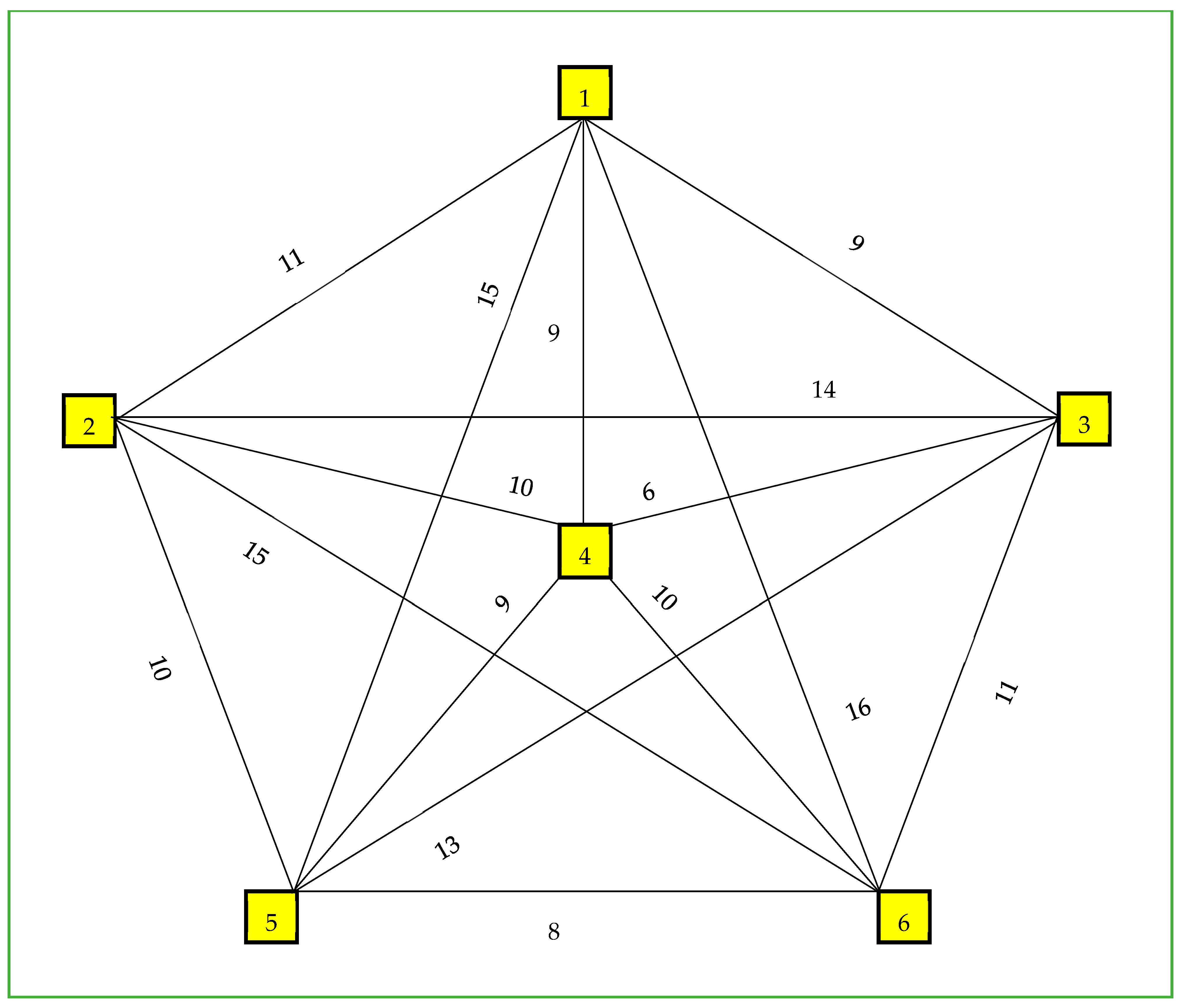
We consider a non-directed 6-node network, as shown in Figure 1. Node 1 is the home city and nodes {2, 3, 4, 5 and 6} are the intermediate nodes. This problem was introduced by Cowen [34] and also considered by Kumar et al. [9].

The corresponding distance matrix for the network in Figure 1 is given in

Table 1. Distance matrix.

	1	2	3	4	5	6
1	∞	11	9	9	15	16
2	11	∞	14	10	10	15
3	9	14	∞	6	13	11
4	9	10	6	∞	9	10
5	15	10	13	9	∞	8
6	16	15	11	10	8	∞

.

5.2. Solution

Initialization. To initialize Algorithm 1 parallel search, consider node 1 as the home city, then connect all nodes $j\in L_0=\left\{2,3,4,5,6\right\}$ to the home city to obtain the following node labels for every element of set $L_0,$ thus $w^{*}{}_{{\left(1,j\right)}^0}=\left\{{11}_{{\left(1,2\right)}^0}, 9_{{\left(1,3\right)}^0}, 9_{{\left(1,4\right)}^0}, {15}_{{\left(1,5\right)}^0}, {16}_{{\left(1,6\right)}^0}\right\}$. These node labels carry the information about partial tours, and respective weights are used as the seed in iteration 1 computations. Set $j\to k$and go to iteration 1.

Algorithm 1 A Labelling Method for the Travelling Salesman Problem

Initialization. For any given network, represent the home city node by 1. The set of all unvisited nodes is given by $L_0=\left\{2, 3,\dots ,n\right\}$. To initialize the algorithm label, all nodes with $w_{{\left(1,j\right)}^z}$ for all $j\in L_0$ are directly connected to the home city (node $1$). Where $w$ is the weight of the shortest path $\left(1,j\right)$ with intermediate nodes $z, \mathrm{initially} z=0$. At the initialization stage, $w^{*}{}_{{\left(1,j\right)}^0}=w_{{\left(1,j\right)}^0}$ Step 1. If $z<\left(n-2\right)$, assign $j\to k, \mathrm{where} k$ is the previous added node, thus changing the label $w^{*}{}_{{\left(1,j\right)}^z}$ to $w^{*}{}_{{\left(1,k\right)}^z}$. For all $j\in L_0$ that is part of the minimum weight label $w^{*}{}_{{\left(1,k\right)}^z}$, label $j$ with $(\infty )$. Otherwise, modify $w^{*}{}_{{\left(1,k\right)}^z}$ to $w_{{\left(1,j\right)}^{z+1}}$ and label $j$ with $w_{{\left(1,j\right)}^{z+1}}$, where $w_{{\left(1,j\right)}^{z+1}}=w^{*}{}_{{\left(1,k\right)}^z}+c_{\left\{k,j\right\}}$. Step 2. For all $j\in L_0$ determine the minimum weight label using the following formula: $w^{*}{}_{{(1,j)}^{z+1}}=Min\{w_{{(1,j)}^{z+1}}\}$, and if node $j$ has ties, consider all of them. Step 3. If $z=\left(n-2\right),$ then go to Step 4. Otherwise, go to Step 1. When $z=\left(n-2\right)$, it follows that all the labels have all elements of $j\in L_0$ as visited nodes; hence, $L_0=\{\varnothing \}$. Step 4. Since $L_1=\{\varnothing \}$, there no remaining nodes to visit; as a result, we are now forced to return back to the home city (node 1). Consider $j\in L^{*}{}_0=\left\{1\right\}$ and go to Steps 1 and 2. Then STOP. Step 5. The tour corresponding to the minimum weight label $w^{*}{}_{{\left(1,j\right)}^{n-2}}$ is the minimum weight tour, where $j\in L^{*}{}_0=\left\{1\right\}$.

Iteration 1. Modify the labels $w^{*}{}_{{\left(1,j\right)}^0}$ to obtain new labels $w_{{\left(1,j\right)}^1}$, as shown in

Table 2. Modified link distances after iteration 1.

${\mathit{w}}^{\mathbf{*}}{}_{{\left(1,\mathit{k}\right)}^0}$	$\mathit{j}=1$	$\mathit{j}=2$	$\mathit{j}=3$	$\mathit{j}=4$	$\mathit{j}=5$	$\mathit{j}=6$
${\mathbf{11}}_{{\left(\mathbf{1},\mathbf{2}\right)}^{\mathbf{0}}}$	∞	∞	${25}_{{\left(1,2,3\right)}^1}$	${21}_{{\left(1,2,4\right)}^1}$	${21}_{{\left(1,2,5\right)}^1}$	${26}_{{\left(1,2,6\right)}^1}$
${\mathbf{9}}_{{\left(\mathbf{1},\mathbf{3}\right)}^{\mathbf{0}}}$	∞	${23}_{{\left(1,3,2\right)}^1}$	∞	${15}_{{\left(1,3,4\right)}^1}$	${22}_{{\left(1,3,5\right)}^1}$	${20}_{{\left(1,3,6\right)}^1}$
${\mathbf{9}}_{{\left(\mathbf{1},\mathbf{4}\right)}^{\mathbf{0}}}$	∞	${19}_{{\left(1,4,2\right)}^1}$	${15}_{{\left(1,4,3\right)}^1}$	∞	${18}_{{\left(1,4,5\right)}^1}$	${19}_{{\left(1,4,6\right)}^1}$
${\mathbf{15}}_{{\left(\mathbf{1},\mathbf{5}\right)}^{\mathbf{0}}}$	∞	${25}_{{\left(1,5,2\right)}^1}$	${28}_{{\left(1,5,3\right)}^1}$	${24}_{{\left(1,5,4\right)}^1}$	∞	${23}_{{\left(1,5,6\right)}^1}$
${\mathbf{16}}_{{\left(\mathbf{1},\mathbf{6}\right)}^{\mathbf{0}}}$	∞	${31}_{{\left(1,6,2\right)}^1}$	${27}_{{\left(1,6,3\right)}^1}$	${26}_{{\left(1,6,4\right)}^1}$	${24}_{{\left(1,6,5\right)}^1}$	∞
${\mathit{w}}^{\mathbf{*}}{}_{{\left(\mathbf{1},\mathit{j}\right)}^{\mathbf{1}}}$	-	${19}_{{\left(1,4,2\right)}^1}$	${15}_{{\left(1,4,3\right)}^1}$	${15}_{{\left(1,3,4\right)}^1}$	${18}_{{\left(1,4,5\right)}^1}$	${19}_{{\left(1,4,6\right)}^1}$

For every column $j\in L_0=\left\{2, 3, 4, 5, 6\right\}$, the minimum weight partial tours are given, as follows: $w^{*}{}_{{\left(1,j\right)}^1}=\left\{{19}_{{\left(1,4,2\right)}^1}, {15}_{{\left(1,4,3\right)}^1}, {15}_{{\left(1,3,4\right)}^1}, {18}_{{\left(1,4,5\right)}^1}, {19}_{{\left(1,4,6\right)}^1}\right\}$. This set of minimum weight partial tours is then used as a seed for the next iteration. Set $j\to k$and go to iteration 2.

Iteration 2. Modify the labels $w^{*}{}_{{\left(1,j\right)}^1}$ to obtain new labels $w_{{\left(1,j\right)}^2}$, as shown in

Table 3. Modified link distances after iteration 2.

${\mathit{w}}^{\mathbf{*}}{}_{{\left(1,\mathit{k}\right)}^1}$	$\mathit{j}=1$	$\mathit{j}=2$	$\mathit{j}=3$	$\mathit{j}=4$	$\mathit{j}=5$	$\mathit{j}=6$
${19}_{{\left(1,4,2\right)}^1}$	∞	∞	${33}_{{\left(1,4,2,3\right)}^2}$	∞	${29}_{{\left(1,4,2,5\right)}^2}$	${34}_{{\left(1,4,2,6\right)}^2}$
${15}_{{\left(1,4,3\right)}^1}$	∞	${29}_{{\left(1,4,3,2\right)}^2}$	∞	∞	${28}_{{\left(1,4,3,5\right)}^2}$	${26}_{{\left(1,4,3,6\right)}^2}$
${15}_{{\left(1,3,4\right)}^1}$	∞	${25}_{{\left(1,3,4,2\right)}^2}$	∞	∞	${24}_{{\left(1,3,4,5\right)}^2}$	${25}_{{\left(1,3,4,6\right)}^2}$
${18}_{{\left(1,4,5\right)}^1}$	∞	${28}_{{\left(1,4,5,2\right)}^2}$	${31}_{{\left(1,4,5,3\right)}^2}$	∞	∞	${26}_{{\left(1,4,5,6\right)}^2}$
${19}_{{\left(1,4,6\right)}^1}$	∞	${34}_{{\left(1,4,6,2\right)}^2}$	${30}_{{\left(1,4,6,3\right)}^2}$	∞	${27}_{{\left(1,4,6,5\right)}^2}$	∞
${\mathit{w}}^{\mathbf{*}}{}_{{\left(\mathbf{1},\mathit{j}\right)}^{\mathbf{2}}}$	-	${25}_{{\left(1,3,4,2\right)}^2}$	${30}_{{\left(1,4,6,3\right)}^2}$	-	${24}_{{\left(1,3,4,5\right)}^2}$	${25}_{{\left(1,3,4,6\right)}^2}$

. For every column $j\in L_0=\left\{2, 3, 5, 6\right\}$, the minimum weight partial tours are given, as follows$: w^{*}{}_{{\left(1,j\right)}^2}=\left\{{25}_{{\left(1,3,4,2\right)}^2}, {10}_{{\left(1,4,6,3\right)}^2}, {24}_{{\left(1,3,4,5\right)}^2}, {25}_{{\left(1,3,4,6\right)}^2}\right\}$. This set of minimum weight partial tours is then used as a seed for the next iteration. Set $j\to k$and go to iteration 3.

Iteration 3. Modify the labels $w^{*}{}_{{\left(1,j\right)}^2}$ to obtain new labels $w_{{\left(1,j\right)}^3}$, as shown in

Table 4. Modified link distances after iteration 3.

${\mathit{w}}^{\mathbf{*}}{}_{{\left(1,\mathit{k}\right)}^2}$	$\mathit{j}=1$	$\mathit{j}=2$	$\mathit{j}=3$	$\mathit{j}=4$	$\mathit{j}=5$	$\mathit{j}=6$
${25}_{{\left(1,3,4,2\right)}^2}$	∞	∞	∞	∞	${35}_{{\left(1,3,4,2,5\right)}^3}$	${40}_{{\left(1,3,4,2,6\right)}^3}$
${30}_{{\left(1,4,6,3\right)}^2}$	∞	${44}_{{\left(1,4,6,3,2\right)}^3}$	∞	∞	${43}_{{\left(1,4,6,3,5\right)}^3}$	∞
${24}_{{\left(1,3,4,5\right)}^2}$	∞	${34}_{{\left(1,3,4,5,2\right)}^3}$	∞	∞	∞	${32}_{{\left(1,3,4,5,6\right)}^3}$
${25}_{{\left(1,3,4,6\right)}^2}$	∞	${40}_{{\left(1,3,4,6,2\right)}^3}$	∞	∞	${33}_{{\left(1,3,4,6,5\right)}^3}$	∞
${\mathit{w}}^{\mathbf{*}}{}_{{\left(\mathbf{1},\mathit{j}\right)}^{\mathbf{3}}}$	-	${34}_{{\left(1,3,4,5,2\right)}^3}$	-	-	${33}_{{\left(1,3,4,6,5\right)}^3}$	${32}_{{\left(1,3,4,5,6\right)}^3}$

. For every column $j\in L_0=\left\{2, 5, 6\right\},$ the minimum weight partial tours are given, as follows: $w^{*}{}_{{\left(1,j\right)}^3}=\left\{{34}_{{\left(1,3,4,5,2\right)}^3}, {33}_{{\left(1,3,4,6,5\right)}^3}, {32}_{{\left(1,3,4,6,5\right)}^3}\right\}$. This set of minimum weight partial tours is then used as a seed for the next iteration. Set $j\to k$and go to iteration 4.

Iteration 4. Modify the labels $w^{*}{}_{{\left(1,j\right)}^3}$ to obtain new labels $w_{{\left(1,j\right)}^4}$, as shown in

Table 5. Modified link distances after iteration 4.

${\mathit{w}}^{\mathbf{*}}{}_{{\left(1,\mathit{k}\right)}^3}$	$\mathit{j}=1$	$\mathit{j}=2$	$\mathit{j}=3$	$\mathit{j}=4$	$\mathit{j}=5$	$\mathit{j}=6$
${34}_{{\left(1,3,4,5,2\right)}^3}$	∞	∞	∞	∞	∞	${49}_{{\left(1,3,4,5,2,6\right)}^4}$
${33}_{{\left(1,3,4,6,5\right)}^3}$	∞	${43}_{{\left(1,3,4,6,5,2\right)}^4}$	∞	∞	∞	∞
${32}_{{\left(1,3,4,5,6\right)}^3}$	∞	${47}_{{\left(1,3,4,5,6,2\right)}^4}$	∞	∞	∞	∞
${\mathit{w}}^{\mathbf{*}}{}_{{\left(\mathbf{1},\mathit{j}\right)}^{\mathbf{4}}}$	-	${43}_{{\left(1,3,4,6,5,2\right)}^4}$	-	-	-	${49}_{{\left(1,3,4,5,2,6\right)}^4}$

. For every column $j\in L_0=\left\{2, 6\right\},$ the minimum weight partial tours are given, as follows: $w^{*}{}_{{\left(1,j\right)}^4}=\left\{{43}_{{\left(1,3,4,6,5,2\right)}^4}, {49}_{{\left(1,3,4,5,2,6\right)}^4}\right\}$. This set of minimum weight partial tours is then used as a seed for the next iteration. Set $j\to k$and go to iteration 5.

Iteration 5. Modify the labels $w^{*}{}_{{\left(1,j\right)}^4}$ to obtain new labels $w_{{\left(1,j\right)}^5}$, as shown in

Table 6. Modified link distances after iteration 5.

${\mathit{w}}^{\mathbf{*}}{}_{{\left(1,\mathit{k}\right)}^4}$	$\mathit{j}=1$	$\mathit{j}=2$	$\mathit{j}=3$	$\mathit{j}=4$	$\mathit{j}=5$	$\mathit{j}=6$
${43}_{{\left(1,3,4,6,5,2\right)}^4}$	${54}_{{\left(1,3,4,6,5,2,1\right)}^5}$	∞	∞	∞	∞	∞
${49}_{{\left(1,3,4,5,2,6\right)}^4}$	${65}_{{\left(1,3,4,5,2,6,1\right)}^5}$	∞	∞	∞	∞	∞
${\mathit{w}}^{\mathbf{*}}{}_{{\left(\mathbf{1},\mathit{j}\right)}^{\mathbf{5}}}$	${54}_{{\left(1,3,4,6,5,2,1\right)}^5}$	-	-	-	-	-

. Now, $j\in L_0=\{\varnothing \}$, and we consider returning back to the home city; thus, we consider $j\in L^{*}{}_0=\left\{1\right\}$, then, the minimum weight optimal tour is given by: $w^{*}{}_{{\left(1,j\right)}^4}=\left\{{54}_{{\left(1,3,4,6,5,2,1\right)}^5}\right\}$.

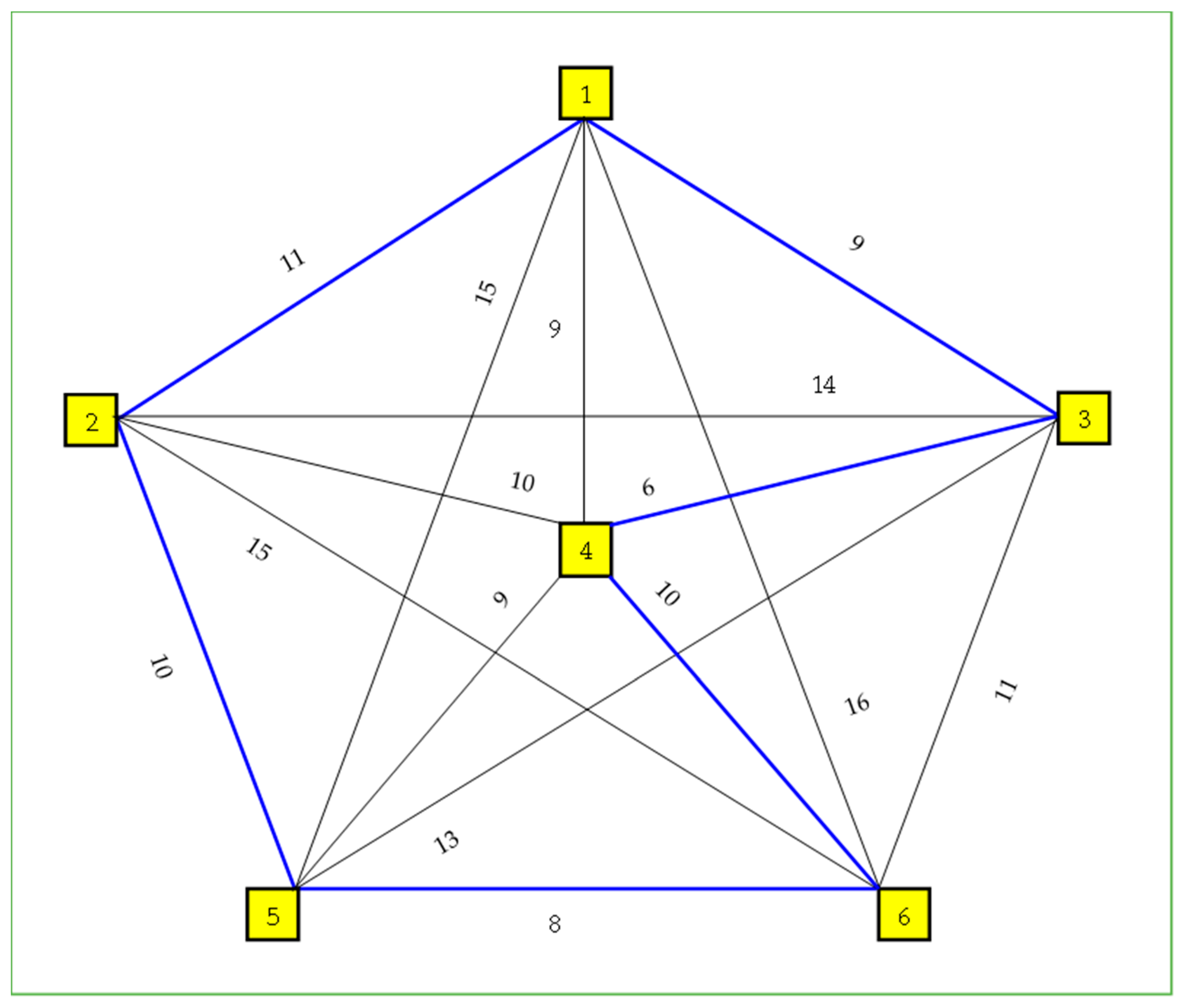
The optimal solution is 1$\to$3$\to$4$\to$6$\to$5$\to$2$\to$1, giving a total distance of 54 units; this solution is the same as the one of Kumar et al. [9]. The above length of 54 units is less than the one obtained by Cowen [34], which is given by 1$\to$2$\to$5$\to$6$\to$3$\to$4$\to$1, giving a total distance of 55 units. The optimal tour is shown in Figure 2.

5.3. Numerical Illustration 2: TSP Problem with Alternative Optimal Tours

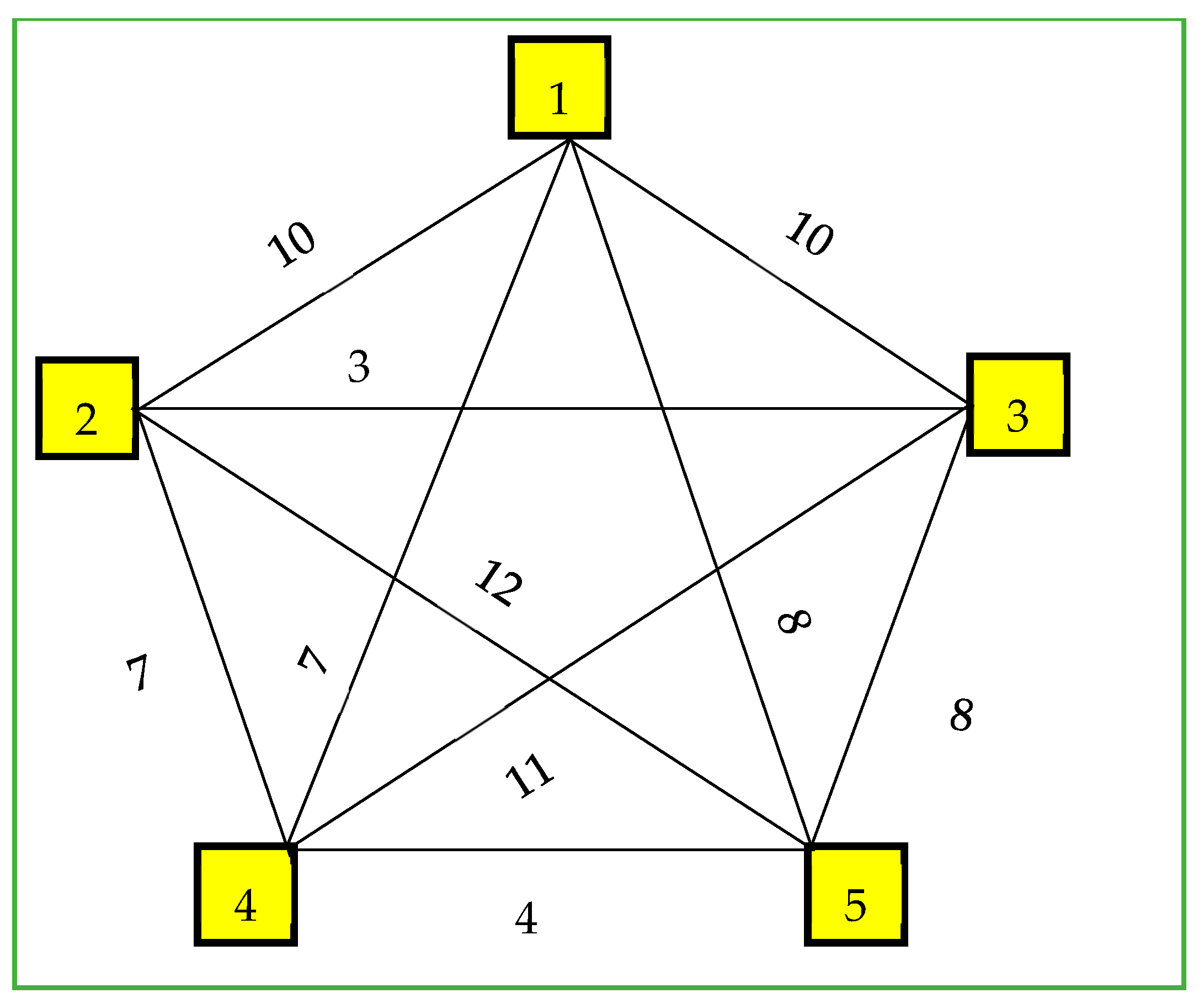
A five-node network is presented in Figure 3, this network is used to demonstrate the ability of the proposed method to determine the alternative optimal tour. The respective distance matrix is shown in

Table 7. Distance matrix.

	1	2	3	4	5
1	∞	10	10	7	8
2	10	∞	3	7	12
3	10	3	∞	11	8
4	7	7	11	∞	4
5	8	12	8	4	∞

. Node 1 is considered as the home city.

Initialization. To initialize the parallel search, consider node 1 as the home city, then connect all nodes $j\in L_0=\left\{2,3,4,5\right\}$ to the home city (node 1) to obtain the following node labels for every element of set $L_0$; thus, $w^{*}{}_{{\left(1,j\right)}^0}=\left\{{10}_{{\left(1,2\right)}^0}, {10}_{{\left(1,3\right)}^0}, 7_{{\left(1,4\right)}^0}, 8_{{\left(1,5\right)}^0}\right\}$. These node labels carry the information about partial tours, and respective weights are used as the seed in iteration 1 computations. Set $j\to k$and go to iteration 1.

Iteration 1. Modify the labels $w^{*}{}_{{\left(1,j\right)}^0}$ to obtain new labels $w_{{\left(1,j\right)}^1}$, as shown in

Table 8. Modified links after iteration 1.

${\mathit{w}}^{\mathbf{*}}{}_{{\left(1,\mathit{k}\right)}^0}$	$\mathit{j}=1$	$\mathit{j}=2$	$\mathit{j}=3$	$\mathit{j}=4$	$\mathit{j}=5$
${10}_{{\left(1,2\right)}^0}$	∞	∞	${13}_{{\left(1,2,3\right)}^1}$	${17}_{{\left(1,2,4\right)}^1}$	${22}_{{\left(1,2,5\right)}^1}$
${10}_{{\left(1,3\right)}^0}$	∞	${13}_{{\left(1,3,2\right)}^1}$	∞	${21}_{{\left(1,3,4\right)}^1}$	${18}_{{\left(1,3,5\right)}^1}$
$7_{{\left(1,4\right)}^0}$	∞	${14}_{{\left(1,4,2\right)}^1}$	${18}_{{\left(1,4,3\right)}^1}$	∞	${11}_{{\left(1,4,5\right)}^1}$
$8_{{\left(1,5\right)}^0}$	∞	${20}_{{\left(1,5,2\right)}^1}$	${16}_{{\left(1,5,3\right)}^1}$	${12}_{{\left(1,5,4\right)}^1}$	∞
${\mathit{w}}^{\mathbf{*}}{}_{{\left(\mathbf{1},\mathit{j}\right)}^{\mathbf{1}}}$	-	${13}_{{\left(1,3,2\right)}^1}$	${13}_{{\left(1,2,3\right)}^1}$	${12}_{{\left(1,5,4\right)}^1}$	${11}_{{\left(1,4,5\right)}^1}$

. For every column $j\in L_0=\left\{2, 3, 4, 5\right\},$ the minimum weight partial tours are given, as follows: $w^{*}{}_{{\left(1,j\right)}^1}=\left\{{13}_{{\left(1,3,2\right)}^1}, {13}_{{\left(1,2,3\right)}^1}, {12}_{{\left(1,5,4\right)}^1}, {11}_{{\left(1,4,5\right)}^1}\right\}$. This set of minimum weight partial tours is then used as a seed for the next iteration. Set $j\to k$and go to iteration 2.

Iteration 2. Modify the labels $w^{*}{}_{{\left(1,j\right)}^1}$ to obtain new labels $w_{{\left(1,j\right)}^2}$, as shown in

Table 9. Modified links after iteration 2.

${\mathit{w}}^{\mathbf{*}}{}_{{\left(1,\mathit{k}\right)}^1}$	$\mathit{j}=1$	$\mathit{j}=2$	$\mathit{j}=3$	$\mathit{j}=4$	$\mathit{j}=5$
${13}_{{\left(1,3,2\right)}^1}$	∞	∞	∞	${20}_{{\left(1,3,2,4\right)}^2}$	${25}_{{\left(1,3,2,5\right)}^2}$
${13}_{{\left(1,2,3\right)}^1}$	∞	∞	∞	${24}_{{\left(1,2,3,4\right)}^2}$	${21}_{{\left(1,2,3,5\right)}^2}$
${12}_{{\left(1,5,4\right)}^1}$	∞	${19}_{{\left(1,5,4,2\right)}^2}$	${23}_{{\left(1,5,4,3\right)}^2}$	∞	∞
${11}_{{\left(1,4,5\right)}^1}$	∞	${23}_{{\left(1,4,5,2\right)}^2}$	${19}_{{\left(1,4,5,3\right)}^2}$	∞	∞
${\mathit{w}}^{\mathbf{*}}{}_{{\left(\mathbf{1},\mathit{j}\right)}^{\mathbf{2}}}$	-	${19}_{{\left(1,5,4,2\right)}^2}$	${19}_{{\left(1,4,5,3\right)}^2}$	${20}_{{\left(1,3,2,4\right)}^2}$	${21}_{{\left(1,2,3,5\right)}^2}$

. For every column $j\in L_0=\left\{2, 3, 4, 5\right\},$ the minimum weight partial tours are given, as follows: $w^{*}{}_{{\left(1,j\right)}^2}=\left\{{19}_{{\left(1,5,4,2\right)}^2}, {19}_{{\left(1,4,5,3\right)}^2}, {20}_{{\left(1,3,2,4\right)}^2}{}_{{\left(1,5,4\right)}^1}, {21}_{{\left(1,2,3,5\right)}^2}\right\}$. This set of minimum weight partial tours is then used as a seed for the next iteration. Set $j\to k$and go to iteration 3.

Iteration 3. Modify the labels $w^{*}{}_{{\left(1,j\right)}^2}$ to obtain new labels $w_{{\left(1,j\right)}^3},$ as shown in

Table 10. Modified links after iteration 3.

${\mathit{w}}^{\mathbf{*}}{}_{{\left(1,\mathit{k}\right)}^2}$	$\mathit{j}=1$	$\mathit{j}=2$	$\mathit{j}=3$	$\mathit{j}=4$	$\mathit{j}=5$
${19}_{{\left(1,5,4,2\right)}^2}$	∞	∞	${22}_{{\left(1,5,4,2,3\right)}^3}$	∞	∞
${19}_{{\left(1,4,5,3\right)}^2}$	∞	${22}_{{\left(1,4,5,3,2\right)}^3}$	∞	∞	∞
${20}_{{\left(1,3,2,4\right)}^2}$	∞	∞	∞	∞	${24}_{{\left(1,3,2,4,5\right)}^3}$
${21}_{{\left(1,2,3,5\right)}^2}$	∞	∞	∞	${25}_{{\left(1,2,3,5,4\right)}^3}$	∞
${\mathit{w}}^{\mathbf{*}}{}_{{\left(\mathbf{1},\mathit{j}\right)}^{\mathbf{3}}}$	-	${22}_{{\left(1,4,5,3,2\right)}^3}$	${22}_{{\left(1,5,4,2,3\right)}^3}$	${25}_{{\left(1,2,3,5,4\right)}^3}$	${24}_{{\left(1,3,2,4,5\right)}^3}$

. For every column $j\in L_0=\left\{2, 3, 4, 5\right\},$ the minimum weight partial tours are given, as follows: $w^{*}{}_{{\left(1,j\right)}^3}=\left\{{22}_{{\left(1,4,5,3,2\right)}^3}, {22}_{{\left(1,5,4,2,3\right)}^3}, {25}_{{\left(1,2,3,5,4\right)}^3}, {24}_{{\left(1,3,2,4,5\right)}^3}\right\}$. This set of minimum weight partial tours is then used as a seed for the next iteration. Set $j\to k$and go to iteration 4.

Iteration 4. Modify the labels $w^{*}{}_{{\left(1,j\right)}^3}$ to obtain new labels $w_{{\left(1,j\right)}^4},$ as shown in

Table 11. Modified links after iteration 4.

${\mathit{w}}^{\mathbf{*}}{}_{{\left(1,\mathit{k}\right)}^3}$	$\mathit{j}=1$	$\mathit{j}=2$	$\mathit{j}=3$	$\mathit{j}=4$	$\mathit{j}=5$
${22}_{{\left(1,4,5,3,2\right)}^3}$	${32}_{{\left(1,4,5,3,2,1\right)}^4}$	∞	∞	∞	∞
${22}_{{\left(1,5,4,2,3\right)}^3}$	${32}_{{\left(1,5,4,2,3,1\right)}^4}$	∞	∞	∞	∞
${25}_{{\left(1,2,3,5,4\right)}^3}$	${32}_{{\left(1,2,3,5,4,1\right)}^4}$	∞	∞	∞	∞
${24}_{{\left(1,3,2,4,5\right)}^3}$	${32}_{{\left(1,3,2,4,5,1\right)}^4}$	∞	∞	∞	∞
${\mathit{w}}^{\mathbf{*}}{}_{{\left(\mathbf{1},\mathit{j}\right)}^{\mathbf{4}}}$	All tours	-	-	-	-

. Now, $j\in L_0=\{\varnothing \}$; consider returning back to the home city (node 1), thus considering $j\in L^{*}{}_0=\left\{1\right\}$. Then, the minimum weight optimal tours are given by: $w^{*}{}_{{\left(1,j\right)}^4}=\left\{{32}_{{\left(1,4,5,3,2,1\right)}^4}, {32}_{{\left(1,5,4,2,3,1\right)}^4}\right\}$.

Optimal tours are given by 1$\to$4$\to$5$\to$3$\to$2$\to$1 or 1$\to$5$\to$4$\to$2$\to$3$\to$1, which give a total distance of 32 units. Figure 4 shows the optimal tours on the network.

6. Conclusions and Future Research

In this paper, we have developed a labelling method that can be used to compute the optimal TSP tour. For any given network with $K$ nodes, the method finds the optimal solution in $K-1$ iterations. Given a network with $M$ optimal solutions, the method is capable of computing all $M$ optimal solutions after K−1 iterations. The method is flexible in that it can be applied to solve both symmetric and asymmetric TSP problems. The computational complexity decreases as the iteration increases, which makes it a very powerful and simple algorithm; thus, the number of operations required per each iteration reduces as the number of iterations approaches K−1. We presented two numerical examples to demonstrate the efficiency of the method, and one numerical illustration from Cowen [34]. The method obtained better solutions compared to the one presented by Cowen [34]. The solution obtained is the same as the one presented by Kumar et al. [9]. The method is designed in such a way that it can be used for teaching purposes. Further studies will include the development of a software for the proposed method so that computational experiments can be conducted using large problem instances, as well as a comparative analysis with other existing methods.

References

1. Sokkappa, P.R. The Cost-Constrained Traveling Salesman Problem. Ph.D. Thesis, Stanford University, Stanford, CA, USA, 1991. [Google Scholar]
2. Dogan, O.; Alkaya, A.F. A novel method for prize collecting traveling salesman problem with time windows. In Intelligent and Fuzzy Techniques for Emerging Conditions and Digital Transformation. In Proceedings of the INFUS 2021 Conference, Istanbul, Turkey, 24–26 August 2021; Springer International Publishing: Cham, Switzerland, 2022; Volume 1, pp. 469–476. [Google Scholar]
3. Venkatesh, P.; Singh, A.; Mallipeddi, R. A multi-start iterated local search algorithm for the maximum scatter traveling salesman problem. In Proceedings of the 2019 IEEE Congress on Evolutionary Computation (CEC), Wellington, New Zealand, 10–13 June 2019; IEEE: New York, NY, USA, 2019; pp. 1390–1397. [Google Scholar]
4. Vincent, F.Y.; Susanto, H.; Jodiawan, P.; Ho, T.W.; Lin, S.W.; Huang, Y.T. A simulated annealing algorithm for the vehicle routing problem with parcel lockers. IEEE Access 2022, 10, 20764–20782. [Google Scholar]
5. Tawanda, T.; Nyamugure, P.; Kumar, S.; Munapo, E. Modified TANYAKUMU Labelling Method to Solve Equality Generalized Travelling Salesman Problem. In Intelligent Computing & Optimization: Proceedings of the 5th International Conference on Intelligent Computing and Optimization 2022 (ICO2022), Hua Hin, Thailand, 27–28 October2022; Springer International Publishing: Cham, Switzerland, 2022; pp. 936–947. [Google Scholar]
6. Kawasaki, M.; Takazawa, K. Improving approximation ratios for the clustered traveling salesman problem. J. Oper. Res. Soc. Jpn. 2020, 63, 60–70. [Google Scholar] [CrossRef]
7. Srivastava, S.S.; Kumar, S.; Garg, R.C.; Sen, P. Generalized travelling salesman problem through n sets of nodes. CORS J. 1969, 7, 97–101. [Google Scholar]
8. Garg, R.C.; Kumar, S.; Dass, P.; Sen, P. Generalized travelling salesman problem through N sets of nodes in a competitive market. AKOR Ahlanf Plan. 1970, 2, 116–120. [Google Scholar]
9. Kumar, S.; Munapo, E.; Lesaoana, M.; Nyamugure, P. A minimum spanning tree based heuristic for the travelling salesman tour. Opsearch 2018, 55, 150–164. [Google Scholar] [CrossRef]
10. Kumar, S.; Munapo, E.; Sigauke, C.; Al-Rabeeah, M. The minimum spanning tree with node index ≤2 Is equivalent to the minimum travelling salesman tour. In Mathematics in Engineering Sciences: Novel Theories, Technologies and Applications; CRC Press: Boca Raton, FL, USA, 2019; Chapter 8; pp. 227–244. [Google Scholar]
11. Munapo, E. A network branch and bound approach for the travelling salesman model. S. Afr. J. Econ. Manag. Sci. 2013, 16, 52–63. [Google Scholar] [CrossRef]
12. Munapo, E. Network Reconstruction—A New Approach to the Traveling Salesman Problem and Complexity. In Intelligent Computing and Optimization. ICO 2019: Advances in Intelligent Systems and Computing, Koh Samui, Thailand, 3–4 October 2019; Vasant, P., Zelinka, I., Weber, G.W., Eds.; Springer: Cham, Switzerland, 2019; Volume 1072. [Google Scholar] [CrossRef]
13. Saksena, J.P.; Kumar, S. The routing problem with ‘K’ specified nodes. Oper. Res. 1966, 14, 909–913. [Google Scholar] [CrossRef]
14. Munapo, E.; Jones, B.C.; Kumar, S. Minimum incoming weight label method and its application in CPM networks. ORiON 2008, 24, 37–48. [Google Scholar] [CrossRef]
15. Kumar, S.; Munapo, E.; Ncube, O.; Sigauke, C.; Nyamugure, P. A minimum weight labelling method for determination of a shortest route in a non-directed network. Int. J. Syst. Assur. Eng. Manag. 2013, 4, 13–18. [Google Scholar] [CrossRef]
16. Tawanda, T. Tawanda’s non- iterative optimal tree algorithm for shortest route problems. Sci. J. Pure Appl. Sci. 2013, 2, 87–94. [Google Scholar]
17. Maposa, D.; Mupondo, N.C.; Tawanda, T. Non-iterative algorithm for finding shortest route. Int. J. Logist. Econ. Glob. 2014, 6, 56–77. [Google Scholar] [CrossRef]
18. Akhand, M.A.H.; Ayon, S.I.; Shahriyar, S.A.; Siddique, N.; Adeli, H. Discrete spider monkey optimization for travelling salesman problem. Appl. Soft Comput. 2019, 86, 105887. [Google Scholar] [CrossRef]
19. Panwar, K.; Deep, K. Discrete grey wolf optimizer for symmetric travelling salesman problem. Appl. Soft Comput. 2021, 105, 1–12. [Google Scholar] [CrossRef]
20. Gharehchopogh, F.S.; Abdollahzadeh, B. An efficient harris hawk optimization algorithm for solving the travelling salesman problem. Clust. Comput. 2022, 25, 1981–2005. [Google Scholar] [CrossRef]
21. Taillard, E.D.; Helsgaun, K. POPMUSIC for travelling salesman problem. Eur. J. Oper. Res. 2018, 272, 420–429. [Google Scholar] [CrossRef]
22. Eremeev, A.V.; Kovalenko, Y.V. A memetic algorithm with optimal recombination for the asymmetric travelling salesman problem. Memetic Comput. 2020, 12, 23–36. [Google Scholar] [CrossRef]
23. Arigliano, A.; Calogiuri, T.; Ghiani, G.; Guerriero, E. A branch and bound algorithm for the time dependent travelling salesman problem. Netw. Int. J. 2018, 72, 382–392. [Google Scholar] [CrossRef]
24. Hatamlou, A. Solving travelling salesman problem using black hole algorithm. Soft Comput. 2018, 22, 8167–8175. [Google Scholar] [CrossRef]
25. Gao, W. New ant colony optimization algorithm for travelling salesman problem. Int. J. Comput. Intell. Syst. 2020, 13, 44–55. [Google Scholar] [CrossRef]
26. Dahan, F.; El Hindi, K.; Mathkour, H.; Alsalman, H. Dynamic flying ant colony optimization for solving the travelling salesman problem. Sensors 2019, 19, 1837. [Google Scholar] [CrossRef]
27. Boccia, M.; Masone, A.; Sforza, A.; Sterle, C. A column and row generation approach for the flying sidekick travelling salesman problem. Transp. Res. Part C 2021, 124, 102913. [Google Scholar] [CrossRef]
28. Gunduz, M.; Aslan, M. DJAYA: A discrete JAYA algorithm for solving the travelling salesman problem. Appl. Soft Comput. 2021, 105, 107275. [Google Scholar] [CrossRef]
29. Zhan, S.; Lin, J.; Zhang, Z.; Zhong, Y. List-Based Simulated Annealing Algorithm for Traveling Salesman Problem. Comput. Intell. Neurosci. 2016, 2016, 1712630. [Google Scholar] [CrossRef] [PubMed]
30. Akhand, M.A.H.; Shill, P.C.; Hossain, M.F.; Junaed, A.B.M.; Murase, K. Producer—Scrounger method to solve travelling salesman problem. Int. J. Intell. Syst. Appl. 2015, 3, 29–36. [Google Scholar]
31. Hussain, A.; Muhammad, Y.S.; Sajid, M.N.; Hussain, I.; Shoukry, A.M.; Gani, S. Genetic algorithm for travelling salesman problem with modified cycle crossover operator. Comput. Intell. Neurosci. 2017, 2017, 7430125. [Google Scholar] [CrossRef]
32. Al-Dallal, A. Using genetic algorithm with combinatorial crossover to solve travelling salesman problem. In Proceedings of the ECTA 2015 7th International Conference on Evolutionary Computation Theory and Applications, Lisbon, Portuga, 12–14 November 2015; Volume 1, pp. 149–156. [Google Scholar]
33. Taha, A.H. Operations Research: An Introduction; Pearson Prentice Hall: Upper Saddle River, NJ, USA, 2017. [Google Scholar]
34. Cowen, L. The Travelling Salesman Problem, Lecture 4, Comp. 260. Advanced Algorithms; Tufts University: Medford, MA, USA, 2011; Available online: http://www.cs.tufts.edu/comp/260/Old/lecture4.pdf (accessed on 5 July 2022).
Figure 1. Six-node network for the travelling salesman problem.
Applsci 13 06417 g001
Figure 2. Optimal solution.
Applsci 13 06417 g002
Figure 3. TSP network with alternative optimal tours.
Applsci 13 06417 g003
Figure 4. Alternative TSP optimal tours.
Applsci 13 06417 g004