Mutual-Inductance Computation between Coaxial Thin Conical Sheet Inductor and the Circular Loop in Air

Featured Application

For the first time the semi-analytical formula for calculating the mutual inductance between the thin conical sheet inductor and the circular loop is given. The coils are coaxial. The potential applications of the presented work are in wireless power systems, and in ultra-broadband applications since the conical shapes limit the effects of the stray capacitance creating the high impedance over a wide bandwidth.

Abstract

The paper describes a new formula for calculating the mutual inductance between a thin conical sheet inductor and a filamentary circular loop, which are coaxial in air. The presented formula is derived semi-analytically using the complete elliptic integrals of the first, second, and third kind, along with the integral term which will be solved numerically. The results are validated using double and single integration methods, as well as the semi-analytical formula. The mutual inductance between a thin cylindrical solenoid and a filamentary circular loop can be obtained using the new formula for the conical coil and circular loop. Presented formulas can be useful in various applications, such as the excitation coil used in electromagnetic-levitation melting, the production of magnetic field homogeneity and broadband RF and wireless power transfer systems that utilize conical inductors. Overall, the paper presents a valuable contribution to the field of inductor design and can be useful in various applications involving conical inductors.

1. Introduction

The paper discusses the challenge of computing the mutual inductance of conventional coils, which has been a topic of research since the time of Maxwell [1]. While analytical solutions in the form of elementary functions exist for linear coils, more complex configurations, such as circular and elliptical coils require solutions in terms of elliptic integrals, Bessel and Struve functions, and hypergeometric convergent series [2,3,4,5,6,7,8]. Numerical methods and commercial software packages are also available, but there is interest in developing analytical and semi-analytical methods for more efficient computations. Reviewing the corresponding literature in physics and electromagnetics, as well as in scientific papers in engineering, one cannot find the calculations of self-inductance and mutual-inductance of the coils of the conical form very often. Recently, in [9], the calculation of the self-inductance of a thin sheet inductor is obtained in the semi-analytical form. Using the same reasoning, in this paper, a semi-analytical formula for calculating the mutual inductance between a thin conical sheet and a filamentary circular loop is given. Coils are coaxial and placed in the air. The thin conical sheet inductor is made of a thin wire with a cross-section that is practically negligible. This assumption also applies to the circular loop.

The new presented method is based on complete elliptical integrals of the first, second, and third kind, along with a term to be solved by numerical integration. As the special case of this new developed formula is the formula for calculating the mutual inductance between the cylindrical solenoid and the filamentary circular loop, the practical applications of the previous mentioned configuration could be interesting in many domains of electromagnetics such as the excitation coil used in electromagnetic-levitation melting, the production of magnetic field homogeneity and the high magnetic field under the cone, which can be used to magnetize a magnetic sheet [10,11,12,13]. The calculation of the previously mentioned coils is useful for conical inductors which are of ideal form for ultra-broadband applications up to 40 GHz since the conical shapes limit the effects of stray capacitances and effectively substitute a series of narrow-band inductors, creating the high impedance over a very wide bandwidth and in wireless power transfer systems that utilize conical inductors [14,15,16,17,18,19,20,21,22,23,24]. In all cases, either the regular or the singular are explained with precise explications. The validation of the presented method is performed using the single and double integration as well as the semi-analytical formula. The Mathematica files with implemented formulas are available upon request.

2. Basic Formulas

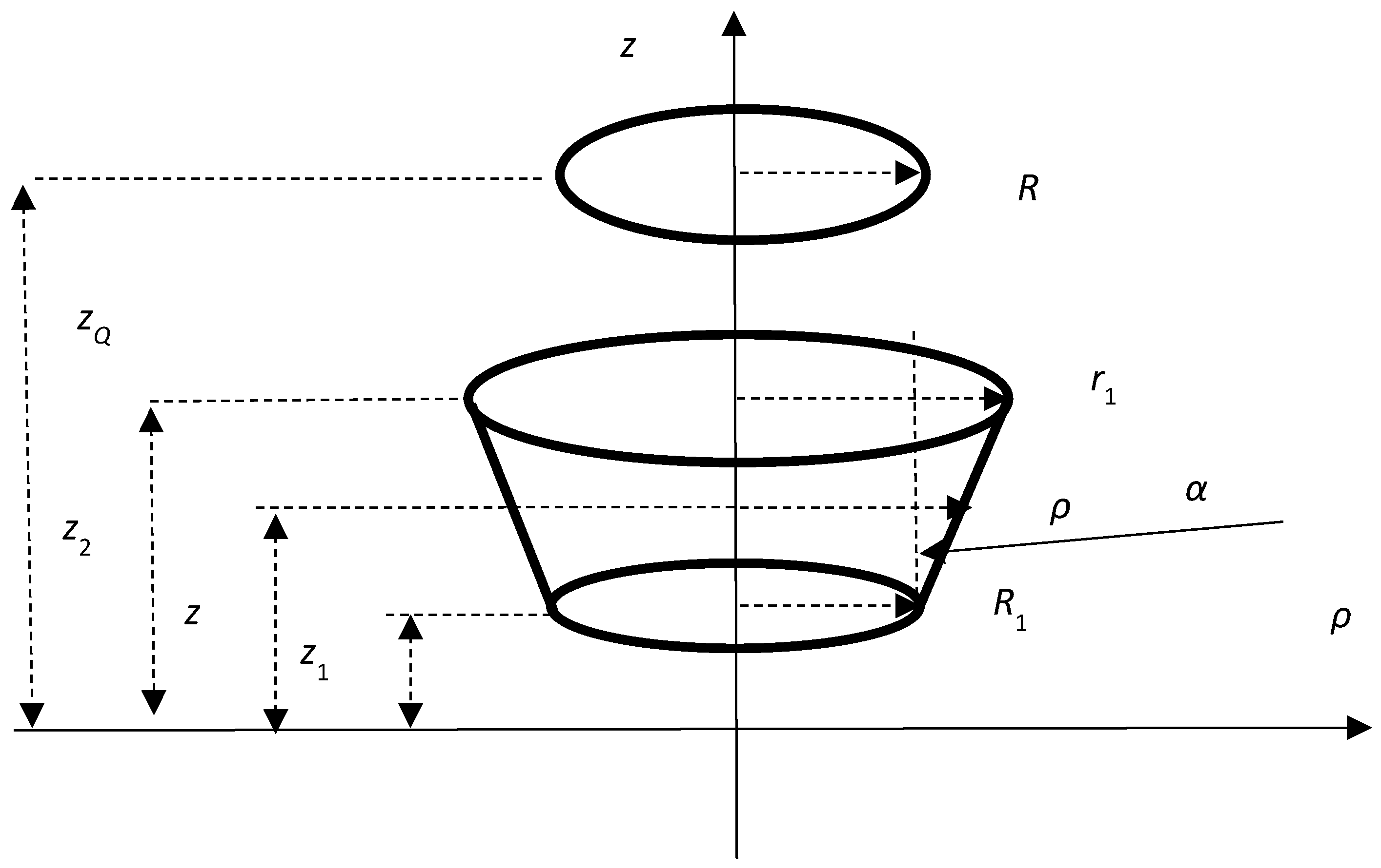
Let us consider a thin conical sheet and a circular loop as shown in Figure 1. The thin conical sheet has the radii of basis $R_1 \mathrm{and} r_1 (R_1>r_1)$. and the axial positions $z_1 \mathrm{and} z_2$, with the number of sheets turns N. The circular loop has the radius R and axial position $z_Q$.

Let us begin the complete analysis for the first case $(R_1>r_1)$, Figure 1.

From Figure 1. one has the following.

$$\frac{R_1-r_1}{z_2-z_1}=\tan \left(\alpha \right)=\eta , R_1=r_1+\eta \left(z_2-z_1\right) \mathrm{or} r_1=R_1-\eta \left(z_2-z_1\right)$$

(1)

$$\frac{z_2-z}{\rho -r_1}=\frac{z_2-z_1}{R_1-r_1}=\frac{1}{\eta } , \rho =r_1-\eta \left(z-z_2\right)=R_1-\eta \left(z-z_1\right)$$

(2)

The mutual inductance between the thin conical sheet inductor and the circular loop can be calculated by the following.

$$M=\frac{{\mu }_{0}N}{z_2-z_1}\underset{0}{\overset{\pi }{{\displaystyle \int }}}\underset{z_1}{\overset{z_2}{{\displaystyle \int }}}\frac{R\rho \cos \left(\theta \right)}{r_0}dzd\theta$$

(3)

with

$$r_0=\sqrt{{\left(R_1-\eta z+\eta z_1\right)}^2-2\left(R_1-\eta z+\eta z_1\right)R\cos \left(\theta \right)+R^2+{\left(z-z_Q\right)}^2}$$

(4)

Equation (3) is obtained from the Neumann formula for the mutual inductance, derived from the magnetic vector potential [7] which is applicable for two coils. By inspection for $R_1=r_1$, Equation (3) becomes [8].

Even though $R_1>r_1 (\eta >0)$ one must use $\rho =R_1-\eta \left(z-z_1\right)$. By the simple verification for $R_1=r_1$ $\left(\eta =0\right)$ the thin conical sheet degenerates to the thin cylindrical solenoid. For this case, the Formula (3) is the formula for calculating the mutual inductance between the thin cylindrical solenoid and the circular loop [8].

Introducing the substitution, $\theta =\pi -2\beta$ in (3) one has the following.

$$M=-\frac{2{\mu }_{0}NR}{z_2-z_1}\underset{0}{\overset{\pi /2}{{\displaystyle \int }}}\underset{z_1}{\overset{z_2}{{\displaystyle \int }}}\frac{\left(R_1-\eta z+\eta z_1\right)\cos \left(2\beta \right)}{r_0}dzd\beta$$

(5)

where

$$r_0=\sqrt{{\left(R_1-\eta z+\eta z_1\right)}^2+2\left(R_1-\eta z+\eta z_1\right)R\cos \left(2\beta \right)+R^2+{\left(z-z_Q\right)}^2}$$

Let us calculate the first integral with respect to z in (5).

$$I_1=\underset{z_1}{\overset{z_2}{{\displaystyle \int }}}\frac{\left(R_1-\eta z+\eta z_1\right)dz}{r_0}$$

(6)

with

$$r_0=\frac{1}{\eta }\sqrt{c_1{t}^2+b_{1}t+a_1}$$

$$c_1={\eta }^2+1$$

$$b_1=2\left[{\eta }^{2}R\cos \left(2\beta \right)-R_1+\eta \left(z_Q-z_1\right)\right]$$

$$a_1={\left[R_1-\eta \left(z_Q-z_1\right)\right]}^2+{\eta }^2{R}^2$$

$${\mathsf{\Delta }}_1=4a_1{c}_1-b_1^2=4{\eta }^2{D}_{10}$$

$$D_{10}=\left\{{\eta }^2{R}^2{\sin }^2\left(2\beta \right)+2R\left[R_1-\eta \left(z_Q-z_1\right)\right]\cos \left(2\beta \right)+{\left[R_1-\eta \left(z_Q-z_1\right)\right]}^2+R^2\right\}$$

$$I_1=\underset{r_1}{\overset{R_1}{{\displaystyle \int }}}\frac{tdt}{\sqrt{c_1{t}^2+b_{1}t+a_1}}$$

(7)

Using [25],

$$\begin{array}{c}{I}_1=\left\{\frac{\sqrt{c_1{R}_1^2+b_1{R}_1+a_1}}{{\eta }^2+1}\right.-\frac{\sqrt{c_1{r}_1^2+b_1{r}_1+a_1}}{{\eta }^2+1}-\frac{{\eta }^{2}R\cos \left(2\beta \right)-R_1+\eta \left(z_1-z_Q\right)}{{\left({\eta }^2+1\right)}^{3/2}}\times \\ \left[arsinh\frac{\eta R\cos \left(2\beta \right)+\eta R_1+z_Q-z_1}{\sqrt{D_{10}}}\right.-\left.arsinh\left.\frac{\eta R\cos \left(2\beta \right)+\eta r_1+z_Q-z_2}{\sqrt{D_{10}}}\right]\right\} \end{array}$$

(8)

Thus, the solution of this integral is obtained in the close form.

Now, the Formula (5) can be given as follows.

$$M=-\frac{2{\mu }_{0}NR}{(z_2-z_1){\left({\eta }^2+1\right)}^{3/2}}\underset{0}{\overset{\pi /2}{{\displaystyle \int }}}V\cos \left(2\beta \right)d\beta$$

(9)

where

$$\begin{array}{c}V=\sqrt{{\eta }^2+1} \left[\sqrt{c_1{R}_1^2+b_1{R}_1+a_1}-\sqrt{c_1{r}_1^2+b_1{r}_1+a_1}\right]-\\ \left[{\eta }^{2}R\cos \left(2\beta \right)-R_1+\eta \left(z_Q-z_1\right)\right]\times \\ \left[arsinh\frac{\eta R\cos \left(2\beta \right)+\eta R_1+z_Q-z_1}{\sqrt{D_{10}}}\right.-\left.arsinh\left.\frac{\eta R\cos \left(2\beta \right)+\eta r_1+z_Q-z_2}{\sqrt{D_{10}}}\right]\right\} \end{array}$$

(10)

Let us solve the following integrals in (9) and (10).

$$I_2=\underset{0}{\overset{\pi /2}{{\displaystyle \int }}}Vcos\left(2\beta \right)d\beta =I_2^{\left(1\right)}+I_2^{\left(2\right)}+I_2^{\left(3\right)}+I_2^{\left(4\right)}$$

(11)

$$I_2^{\left(1\right)}=\sqrt{{\eta }^2+1}\underset{0}{\overset{\pi /2}{{\displaystyle \int }}}\sqrt{c{R}_1^2+b{R}_1+a}cos\left(2\beta \right)d\beta =\sqrt{{\eta }^2+1}\underset{0}{\overset{\pi /2}{{\displaystyle \int }}}\sqrt{T_1}\cos \left(2\beta \right)d\beta$$

(12)

$$T_1=c_1{R}_1^2+b_1{R}_1+a_1={\eta }^2\left[{\left(R+R_1\right)}^2+{\left(z_Q-z_1\right)}^2-4R{R}_1 {\sin }^2\left(\beta \right)\right]$$

$$I_2^{\left(1\right)}=\sqrt{{\eta }^2+1}\sqrt{{\eta }^2\left[{\left(R+R_1\right)}^2+{\left(z_Q-z_1\right)}^2\right]}\underset{0}{\overset{\pi /2}{{\displaystyle \int }}}{\mathsf{\Delta }}_1(1-2{\sin }^2\left(\beta \right))d\beta$$

$${\mathsf{\Delta }}_1=\sqrt{1-k_1^2{\sin }^2\left(\beta \right)} , k_1^2=\frac{4R{R}_1}{{\left(R+R_1\right)}^2+{\left(z_Q-z_1\right)}^2}$$

(13)

Using [25] one obtains the following.

$$\begin{array}{c}{I}_2^{\left(1\right)}=2\eta \sqrt{{\eta }^2+1}\frac{\sqrt{R{R}_1}}{k_1}\underset{0}{\overset{\frac{\pi }{2}}{{\displaystyle \int }}}{\mathsf{\Delta }}_1(1-2{\sin }^2\left(\beta \right))d\beta =\\ 2\eta \sqrt{{\eta }^2+1}\frac{\sqrt{R{R}_1}}{3k_1^3}\left\{\left(2k_1^2-2\right)K\left(k_1\right)+\right.\left.\left(2-k_1^2\right)E\left(k_1\right)\right\}\end{array}$$

or

$$I_2^{\left(1\right)}=2\eta \sqrt{{\eta }^2+1}\frac{\sqrt{R{R}_1}}{3k_1^3}\left\{\left(2k_1^2-2\right)K\left(k_1\right)+\left.\left(2-k_1^2\right)E\left(k_1\right)\right\} \right.$$

(14)

This solution is obtained in the close form where $K\left(k_1\right) \mathrm{and} E\left(k_1\right)$ are the complete elliptic integrals of the first and second kind [25,26].

Similarly, the solution of the next integral,

$$I_2^{\left(2\right)}=-\sqrt{{\eta }^2+1}\underset{0}{\overset{\frac{\pi }{2}}{{\displaystyle \int }}}\sqrt{c{r}_1^2+b{r}_1+a}\cos \left(2\beta \right)d\beta$$

(15)

is also obtained in the close form as follows,

$$I_2^{\left(2\right)}=-2\eta \sqrt{{\eta }^2+1}\frac{\sqrt{R{r}_1}}{3k_2^3}\left\{\left(2k_2^2-2\right)K\left(k_2\right)+\left.\left(2-k_2^2\right)E\left(k_2\right)\right\} \right.$$

(16)

with

$$k_2^2=\frac{4R{r}_1}{{\left(R+r_1\right)}^2+{\left(z_2-z_Q\right)}^2}$$

The next integral is

$$\begin{array}{c}{I}_2^{\left(3\right)}=-\underset{0}{\overset{\frac{\pi }{2}}{{\displaystyle \int }}}\left[{\eta }^{2}R\cos \left(2\beta \right)-R_1+\eta \left(z_Q-z_1\right)\right]\times \\ \cos \left(2\beta \right)\mathrm{arsinh}\frac{\eta R\cos \left(2\beta \right)+\eta R_1+z_Q-z_1}{\sqrt{D_{10}}}d\beta \end{array}$$

(17)

or

$$\begin{array}{c}{I}_2^{\left(3\right)}=-\frac{{\eta }^{2}R}{2}\underset{0}{\overset{\frac{\pi }{2}}{{\displaystyle \int }}}\mathrm{arsinh}\frac{\eta R\cos \left(2\beta \right)+\eta R_1+z_Q-z_1}{\sqrt{D_{10}}}d\beta -\\ \frac{1}{2}\underset{0}{\overset{\frac{\pi }{2}}{{\displaystyle \int }}}\left\{{\eta }^{2}R\cos \left(4\beta \right)-2\left[R_1-\eta \left(z_Q-z_1\right)\right]\cos \left(2\beta \right)\right\}\mathrm{arsinh}\frac{\eta R\cos \left(2\beta \right)+\eta R_1+z_Q-z_1}{\sqrt{D_{10}}}d\beta =\\ -\frac{1}{2}\underset{0}{\overset{\frac{\pi }{2}}{{\displaystyle \int }}}\left\{{\eta }^{2}R\cos \left(4\beta \right)-2\left[R_1-\eta \left(z_Q-z_1\right)\right]\cos \left(2\beta \right)\right\}\mathrm{arsinh}\frac{\eta R\cos \left(2\beta \right)+\eta R_1+z_Q-z_1}{\sqrt{D_{10}}}d\beta =\\ -\frac{{\eta }^{2}R}{2}{J}_{10} \end{array}$$

(18)

where

$$J_{10}=\underset{0}{\overset{\frac{\pi }{2}}{{\displaystyle \int }}}arsinh\frac{\eta R\cos \left(2\beta \right)+\eta R_1+z_Q-z_1}{\sqrt{D_{10}}}d\beta$$

This integral $J_{10}$ does not have the analytical solution, so it must be solved numerically. The kernel function of this integral is the continuous function of the interval of integration.

Let us solve this integral by partial integration (Appendix A).

Thus, the solution is

$$\begin{array}{c}{I}_2^{\left(3\right)}=-\frac{{\eta }^{2}R}{2}{J}_{10}+\frac{\eta \sqrt{{\eta }^2+1}\sqrt{R{R}_1}}{12k_1^3}\left\{\left[3\left(a_{22}+a_{33}\right)k_1^4-\left(6a_{22}+8\right)k_1^2+8\right]\right.K\left(k_1\right)+\\ \left[\left(6a_{22}+4\right)k_2^2-8\right]\left.E\left(k_1\right)\right\}+\frac{k_1\eta \sqrt{{\eta }^2+1}\sqrt{R{R}_1}}{4}\left[\frac{V_1}{1-p_1}\Pi \left(h_1,k_1\right)+\frac{V_2}{1-p_2}\Pi \left(h_2,k_1\right)\right] \end{array}$$

(19)

Similarly,

$$I_2^{\left(4\right)}=\underset{0}{\overset{\frac{\pi }{2}}{{\displaystyle \int }}}\left[{\eta }^{2}R\cos \left(2\beta \right)-R_1+\eta \left(z_Q-z_1\right)\right]\cos \left(2\beta \right)\mathrm{arsinh}\frac{\eta R\cos \left(2\beta \right)+\eta R_1+z_Q-z_2}{\sqrt{D_{10}}}d\beta$$

(20)

can be obtained as follows (Appendix A),

$$\begin{array}{c}{I}_2^{\left(4\right)}=\frac{{\eta }^{2}R}{2}{J}_{20}+\frac{\eta \sqrt{{\eta }^2+1}\sqrt{R{r}_1}}{12k_2^3}\left\{\left[3\left(a_{222}+a_{333}\right)k_2^4-\left(6a_{222}+8\right)k_2^2+8\right]\right.K\left(k_2\right)+\\ \left[\left(6a_{222}+4\right)k_2^2-8\right]\left.E\left(k_2\right)\right\}+\frac{k_2\eta \sqrt{{\eta }^2+1}\sqrt{R{r}_1}}{4}\left[\frac{V_3}{1-p_3}\Pi \left(h_3,k_2\right)+\frac{V_4}{1-p_4}\Pi \left(h_4,k_2\right)\right]\end{array}$$

(21)

where

$$J_{20}=\underset{0}{\overset{\frac{\pi }{2}}{{\displaystyle \int }}}\mathrm{arsinh}\frac{\eta R\cos \left(2\beta \right)+\eta R_1+z_Q-z_2}{\sqrt{D_{10}}}d\beta$$

Finally, from (9), (14), (16), (19) and (21) the mutual inductance between the thin conical sheet and the circular loop can be calculated in the semi-analytical form as follows,

$$M=-\frac{2{\mu }_{0}NR}{(z_2-z_1){\left({\eta }^2+1\right)}^{\frac{3}{2}}}{V}_0$$

(22)

where

$$\begin{array}{c}{V}_0=-\frac{{\eta }^{2}R}{2}{J}_0-\frac{\eta \sqrt{{\eta }^2+1}\sqrt{R{R}_1}}{12k_1^3}\left\{\left[3\left(a_{22}+a_{33}\right)k_1^4-\left(6a_{22}+8\right)k_1^2+8\right]\right.K\left(k_1\right)+\\ \left[\left(6a_{22}+4\right)k_1^2-8\right]\left.E\left(k_1\right)\right\}-\eta \sqrt{{\eta }^2+1}\frac{\sqrt{R{R}_1}}{12k_1^3}\left\{\left(16k_1^2-16\right)K\left(k_1\right)+\right.\\ \left.\left(16-8k_1^2\right)E\left(k_1\right)\right\}+\frac{\eta \sqrt{{\eta }^2+1}\sqrt{R{r}_1}}{12k_2^3}\left\{\left[3\left(a_{222}+a_{333}\right)k_2^4-\left(6a_{222}+8\right)k_2^2+8\right]\right.K\left(k_2\right)+\\ \left[\left(6a_{222}+4\right)k_2^2-8\right]\left.E\left(k_2\right)\right\}+\eta \sqrt{{\eta }^2+1}\frac{\sqrt{R{r}_1}}{12k_2^3}\times \\ \left\{\left(16k_2^2-16\right)K\left(k_2\right)+\left.\left(16-8k_2^2\right)E\left(k_2\right)\right\}-\right.\frac{k_1\eta \sqrt{{\eta }^2+1}\sqrt{R{R}_1}}{4}\times \\ \left[\frac{V_1}{1-p_1}\Pi \left(h_1,k_1\right)+\frac{V_2}{1-p_2}\Pi \left(h_2,k_1\right)\right]+\frac{k_2\eta \sqrt{{\eta }^2+1}\sqrt{R{r}_1}}{4}+\\ \left[\frac{V_3}{1-p_3}\Pi \left(h_3,k_2\right)+\frac{V_4}{1-p_4}\Pi \left(h_4,k_2\right)\right] \end{array}$$

(23)

$$J_0=J_{10}-J_{20}$$

All parameters in (23) can be found in Appendix A.

Thus, the general solution of Equation (22) with (23) is expressed by the complete elliptic integrals K(k), E(k) and Π(h, k) as well as one term J₀ which must be solved numerically.

2.1. Singular Cases

The Equation (22) with (23) can be directly applied for the general cases. It is possible to have in (23) four singular cases so that one must do some corrections to overcome these problems. The singular cases appear when coils are in contact or overlap. In these cases, some parameters obtain the values for which the elliptical integrals begin infinite, so they must be considered particularly.

2.1.1. $p_1=p_3=-1$

From (23), one can see that for $p_1=-1$ the singular case appears and $A=B$ so that so that the following is true.

$$\begin{array}{c}\frac{\left[A\cos \left(2\beta \right)+B\right]}{\left[\cos \left(2\beta \right)-p_1\right]\left[\cos \left(2\beta \right)-p_2\right]}=\frac{A\left[cos\left(2\beta \right)+1\right]}{\left[\cos \left(2\beta \right)+1\right]\left[\cos \left(2\beta \right)-p_2\right]}=\frac{A}{\cos \left(2\beta \right)-p_2}=\\ \frac{A}{1-p_2}\frac{1}{1-h_2{\sin }^2\left(\beta \right)} \end{array}$$

(24)

In (23), the singularity appears for $p_3=-1$ and $C=D$ so that so that the following is true.

$$\begin{array}{c}\frac{\left[C\cos \left(2\beta \right)+D\right]}{\left[\cos \left(2\beta \right)-p_3\right]\left[\cos \left(2\beta \right)-p_4\right]}=\frac{C\left[cos\left(2\beta \right)+1\right]}{\left[\cos \left(2\beta \right)+1\right]\left[\cos \left(2\beta \right)-p_4\right]}=\frac{C}{\cos \left(2\beta \right)-p_4}=\\ \frac{C}{1-p_4}\frac{1}{1-h_4{\sin }^2\left(\beta \right)} \end{array}$$

(25)

From (24) and (25), it is obvious that the complete elliptic integrals of the third kind $\Pi \left(h_1,k_1\right)$ and $\Pi \left(h_3,k_3\right)$ will vanish.

Thus, (23) begins as the following.

$$\begin{array}{c}{V}_0=-\frac{{\eta }^{2}R}{2}{J}_0-\frac{\eta \sqrt{{\eta }^2+1}\sqrt{R{R}_1}}{12k_1^3}\left\{\left[3\left(a_{22}+a_{33}\right)k_1^4-\left(6a_{22}+8\right)k_1^2+8\right]\right.K\left(k_1\right)+\\ \left[\left(6a_{22}+4\right)k_1^2-8\right]\left.E\left(k_1\right)\right\}-\eta \sqrt{{\eta }^2+1}\frac{\sqrt{R{R}_1}}{12k_1^3}\left\{\left(16k_1^2-16\right)K\left(k_1\right)+\right.\\ \left.\left(16-8k_1^2\right)E\left(k_1\right)\right\}+\frac{\eta \sqrt{{\eta }^2+1}\sqrt{R{r}_1}}{12k_2^3}\left\{\left[3\left(a_{222}+a_{333}\right)k_2^4-\left(6a_{222}+8\right)k_2^2+8\right]\right.K\left(k_2\right)+\\ \left[\left(6a_{222}+4\right)k_2^2-8\right]\left.E\left(k_2\right)\right\}+\eta \sqrt{{\eta }^2+1}\frac{\sqrt{R{r}_1}}{12k_2^3}\left\{\left(16k_2^2-16\right)\right.K\left(k_2\right)+\left.\left(16-8k_2^2\right)E\left(k_2\right)\right\}-\\ \frac{k_1\eta \sqrt{{\eta }^2+1}\sqrt{R{R}_1}}{4}\frac{A}{1-p_2}\Pi \left(h_2,k_1\right)+\frac{k_2\eta \sqrt{{\eta }^2+1}\sqrt{R{r}_1}}{4}\frac{C}{1-p_4}\Pi \left(h_4,k_2\right) \end{array}$$

(26)

2.1.2. $p_1=p_3=1$

From (23), one can see that for $p_1=1$ the singular case appears and $A=-B$ so that so that the following is true.

$$\begin{array}{c}\frac{\left[A\cos \left(2\beta \right)+B\right]}{\left[\cos \left(2\beta \right)-p_1\right]\left[\cos \left(2\beta \right)-p_2\right]}=\frac{A\left[cos\left(2\beta \right)-1\right]}{\left[\cos \left(2\beta \right)-1\right]\left[\cos \left(2\beta \right)-p_2\right]}=\frac{A}{\cos \left(2\beta \right)-p_2}=\\ \frac{A}{1-p_2}\frac{1}{1-h_2{\sin }^2\left(\beta \right)} \end{array}$$

(27)

In (23) the singularity appears for $p_3=1$ and $C=-D$ so that so that the following is true.

$$\begin{array}{c}\frac{\left[C\cos \left(2\beta \right)+D\right]}{\left[\cos \left(2\beta \right)-p_3\right]\left[\cos \left(2\beta \right)-p_4\right]}=\frac{C\left[cos\left(2\beta \right)-1\right]}{\left[\cos \left(2\beta \right)-1\right]\left[\cos \left(2\beta \right)-p_4\right]}=\frac{C}{\cos \left(2\beta \right)-p_4}=\\ \frac{C}{1-p_4}\frac{1}{1-h_4{\sin }^2\left(\beta \right)} \end{array}$$

(28)

From (27) and (28), it is obvious that the complete elliptic integrals of the third kind $\Pi \left(h_1,k_1\right)$ and $\Pi \left(h_3,k_3\right)$ will vanish.

Thus, for this case we use (26).

2.1.3. $p_2=p_4=-1$

From (23) one can see that case that for $p_2=-1$ the singular case appears and $A=B$ so that so that the following is true.

$$\begin{array}{c}\frac{\left[A\cos \left(2\beta \right)+B\right]}{\left[\cos \left(2\beta \right)-p_1\right]\left[\cos \left(2\beta \right)-p_2\right]}=\frac{A\left[cos\left(2\beta \right)+1\right]}{\left[\cos \left(2\beta \right)+1\right]\left[\cos \left(2\beta \right)-p_1\right]}=\frac{A}{\cos \left(2\beta \right)-p_1}=\\ \frac{A}{1-p_1}\frac{1}{1-h_1{\sin }^2\left(\beta \right)} \end{array}$$

(29)

In (23) the singularity appears for $p_4=-1$ and $C=D$ so that so that the following is true.

$$\begin{array}{c}\frac{\left[C\cos \left(2\beta \right)+D\right]}{\left[\cos \left(2\beta \right)-p_3\right]\left[\cos \left(2\beta \right)-p_4\right]}=\frac{C\left[cos\left(2\beta \right)+1\right]}{\left[\cos \left(2\beta \right)+1\right]\left[\cos \left(2\beta \right)-p_3\right]}=\frac{C}{\cos \left(2\beta \right)-p_3}=\\ \frac{C}{1-p_3}\frac{1}{1-h_3{\sin }^2\left(\beta \right)} \end{array}$$

(30)

From (34) and (35), one can see that the complete elliptic integrals of the third kind $\Pi \left(h_2,k_1\right)$ and $\Pi \left(h_4,k_3\right)$ will vanish.

Thus, (23) begins as the following.

$$\begin{array}{c}{V}_0=-\frac{{\eta }^{2}R}{2}{J}_0-\frac{\eta \sqrt{{\eta }^2+1}\sqrt{R{R}_1}}{12k_1^3}\left\{\left[3\left(a_{22}+a_{33}\right)k_1^4-\left(6a_{22}+8\right)k_1^2+8\right]\right.K\left(k_1\right)+ \\ \left[\left(6a_{22}+4\right)k_1^2-8\right]\left.E\left(k_1\right)\right\}-\eta \sqrt{{\eta }^2+1}\frac{\sqrt{R{R}_1}}{12k_1^3}\left\{\left(16k_1^2-16\right)K\left(k_1\right)+\right.\\ \left.\left(16-8k_1^2\right)E\left(k_1\right)\right\}+\frac{\eta \sqrt{{\eta }^2+1}\sqrt{R{r}_1}}{12k_2^3}\left\{\left[3\left(a_{222}+a_{333}\right)k_2^4-\left(6a_{222}+8\right)k_2^2+8\right]\right.K\left(k_2\right)+\\ \left[\left(6a_{222}+4\right)k_2^2-8\right]\left.E\left(k_2\right)\right\}+\eta \sqrt{{\eta }^2+1}\frac{\sqrt{R{r}_1}}{12k_2^3}\left\{\left(16k_2^2-16\right)\right.K\left(k_2\right)+\left.\left(16-8k_2^2\right)E\left(k_2\right)\right\}-\\ \frac{k_1\eta \sqrt{{\eta }^2+1}\sqrt{R{R}_1}}{4}\frac{A}{1-p_1}\Pi \left(h_1,k_1\right)+\frac{k_2\eta \sqrt{{\eta }^2+1}\sqrt{R{r}_1}}{4}\frac{C}{1-p_3}\Pi \left(h_3,k_2\right) \end{array}$$

(31)

2.1.4. $p_2=p_4=1$

From (23) one can see that case that for $p_2=1$ the singular case appears and $A=-B$ so that so that the following is true.

$$\begin{array}{c}\frac{\left[A\cos \left(2\beta \right)+B\right]}{\left[\cos \left(2\beta \right)-p_1\right]\left[\cos \left(2\beta \right)-p_2\right]}=\frac{A\left[cos\left(2\beta \right)-1\right]}{\left[\cos \left(2\beta \right)-1\right]\left[\cos \left(2\beta \right)-p_1\right]}=\frac{A}{\cos \left(2\beta \right)-p_1}=\\ \frac{A}{1-p_1}\frac{1}{1-h_1{\sin }^2\left(\beta \right)} \end{array}$$

(32)

In (23) the singularity appears for $p_4=-1$ and $C=-D$ so that so that the following is true.

$$\begin{array}{c}\frac{\left[C\cos \left(2\beta \right)+D\right]}{\left[\cos \left(2\beta \right)-p_3\right]\left[\cos \left(2\beta \right)-p_4\right]}=\frac{C\left[\cos \left(2\beta \right)+1\right]}{\left[\cos \left(2\beta \right)+1\right]\left[\cos \left(2\beta \right)-p_3\right]}=\frac{C}{\cos \left(2\beta \right)-p_3}=\\ \frac{C}{1-p_3}\frac{1}{1-h_3{\sin }^2\left(\beta \right)} \end{array}$$

(33)

From (32) and (33), one can see that the complete elliptic integrals of the third kind $\Pi \left(h_2,k_1\right)$ and $\Pi \left(h_4,k_2\right)$ will vanish. Thus, for this case we use (31).

From this detailed analysis, all partial singular cases can be found in the previous discussed cases.

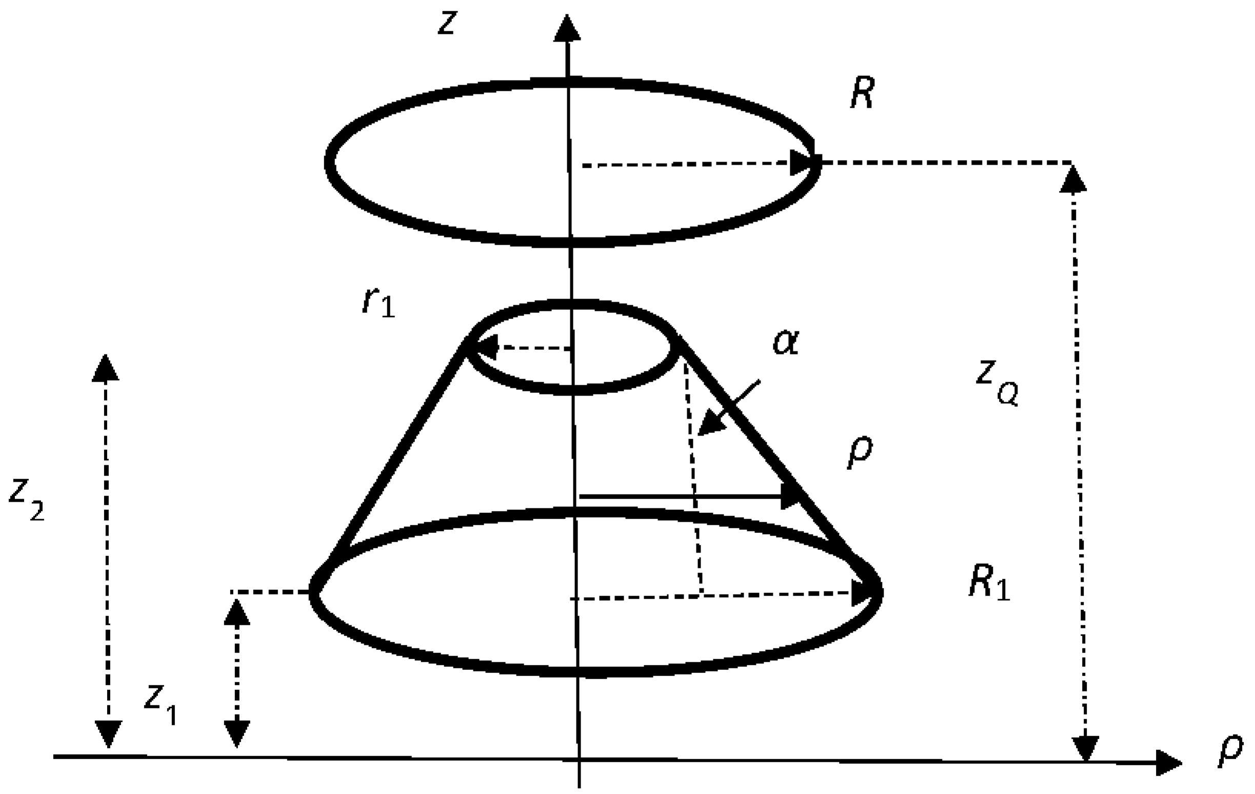
2.2. Case $r_1>R_1$

Now, let us consider a thin conical sheet and a circular loop as shown in Figure 2. The thin conical sheet has the radii of basis $R_1 \mathrm{and} r_1 (r_1>R_1)$ and the axial positions $z_1 \mathrm{and} z_2$, with the number of sheets turns N. The circular loop has the radius R and radial position $z_Q$.

In this case of $r_1>R_1$, one can use the same reasoning as in the previous case.

From Figure 2, we have the following.

$$\frac{r_1-R_1}{z_2-z_1}=\tan \left(\alpha \right)=\eta , r_1=R_1+\eta \left(z_2-z_1\right)$$

(34)

$$\frac{z-z_1}{\rho -R_1}=\frac{z_2-z_1}{r_1-R_1}=\frac{1}{\eta } , \rho =R_1+\eta \left(z-z_1\right)$$

(35)

The mutual inductance can be calculated as follows.

$$M=\frac{{\mu }_{0}N}{z_2-z_1}\underset{0}{\overset{\pi }{{\displaystyle \int }}}\underset{z_1}{\overset{z_2}{{\displaystyle \int }}}\frac{R\rho \cos \left(\theta \right)}{r_0}dzd\theta =\frac{{\mu }_{0}N}{z_2-z_1}\underset{0}{\overset{\pi }{{\displaystyle \int }}}\underset{z_1}{\overset{z_2}{{\displaystyle \int }}}\frac{R\left(R_1+\eta z-\eta z_1\right)\cos \left(\theta \right)}{r_0}dzd\theta$$

(36)

with

$$r_0=\sqrt{{\left(R_1+\eta z-\eta z_1\right)}^2-2\left(R_1+\eta z-\eta z_1\right)R\cos \left(\theta \right)+R^2+{\left(z-z_Q\right)}^2}$$

(37)

Introducing the substitution, $\theta =\pi -2\beta$ in (36) one has the following.

$$M=-\frac{2{\mu }_{0}NR}{z_2-z_1}\underset{0}{\overset{\pi /2}{{\displaystyle \int }}}\underset{z_1}{\overset{z_2}{{\displaystyle \int }}}\frac{\left(R_1+\eta z-\eta z_1\right)\cos \left(2\beta \right)}{r_0}dzd\beta$$

(38)

with

$$r_0=\sqrt{{\left(R_1+\eta z-\eta z_1\right)}^2+2\left(R_1+\eta z-\eta z_1\right)R\cos \left(2\beta \right)+R^2+{\left(z-z_Q\right)}^2}$$

The mutual inductance can be calculated by the double integration (38). Following the procedures as in Section 2.1, after the first integration over the variable z, one has the following.

$$M=\frac{2{\mu }_{0}NR}{(z_2-z_1){\left({\eta }^2+1\right)}^{3/2}}\underset{0}{\overset{\pi /2}{{\displaystyle \int }}}V\cos \left(2\beta \right)d\beta$$

(39)

where

$$\begin{array}{c}V=\sqrt{{\eta }^2+1} \left[\sqrt{c_0{R}_1^2+b_0{R}_1+a_0}-\sqrt{c_0{r}_1^2+b_0{r}_1+a_0}\right]-\left[{\eta }^{2}R\cos \left(2\beta \right)-R_1-\eta \left(z_Q-z_1\right)\right]\\ \times \left[\mathrm{arsinh}\frac{\eta R\cos \left(2\beta \right)+\eta R_1-z_Q+z_1}{\sqrt{D_{20}}}\right.-\left.\mathrm{arsinh}\frac{\eta R\cos \left(2\beta \right)+\eta r_1-z_Q+z_2}{\sqrt{D_{20}}}\right] \end{array}$$

(40)

$$c_0={\eta }^2+1$$

$$b_0=2\left[{\eta }^{2}R\cos \left(2\beta \right)-R_1-\eta \left(z_Q-z_1\right)\right]$$

$$a_0={\left[R_1+\eta \left(z_Q-z_1\right)\right]}^2+{\eta }^2{R}^2$$

$${\mathsf{\Delta }}_0=4{\eta }^2{D}_{00}$$

$$D_{20}=\left\{{\eta }^2{R}^2{\sin }^2\left(2\beta \right)+2R\left[R_1+\eta \left(z_Q-z_1\right)\right]\cos \left(2\beta \right)+{\left[R_1+\eta \left(z_Q-z_1\right)\right]}^2+R^2\right\}$$

Finally, using the same procedures as in Section 2.1 after the second integration the mutual inductance in the semi-analytical form is given as follows.

$$M=\frac{2{\mu }_{0}NR}{(z_2-z_1){\left({\eta }^2+1\right)}^{3/2}}{V}_{00}$$

(41)

with

$$\begin{array}{c}{V}_{00}=-\frac{{\eta }^{2}R}{2}{J}_{00}-\frac{\eta \sqrt{{\eta }^2+1}\sqrt{R{R}_1}}{12k_1^3}\left\{\left[3\left(d_2+d_3\right)k_1^4-\left(6d_2+8\right)k_1^2+8\right]\right.K\left(k_1\right)+\\ \left[\left(6d_2+4\right)k_1^2-8\right]\left.E\left(k_1\right)\right\}+\left|\eta \right|\sqrt{{\eta }^2+1}\frac{\sqrt{R{R}_1}}{12k_1^3}\left\{\left(16k_1^2-16\right)K\left(k_1\right)+\right.\\ \left.\left(16-8k_1^2\right)E\left(k_1\right)\right\}+\frac{\eta \sqrt{{\eta }^2+1}\sqrt{R{r}_1}}{12k_2^3}\left\{\left[3\left(d_{22}+d_{33}\right)k_2^4-\left(6d_{22}+8\right)k_2^2+8\right]\right.K\left(k_2\right)+\\ \left[\left(6d_{22}+4\right)k_2^2-8\right]\left.E\left(k_2\right)\right\}-\left|\eta \right|\sqrt{{\eta }^2+1}\frac{\sqrt{R{r}_1}}{12k_2^3}\times \\ \left\{\left(16k_2^2-16\right)K\left(k_2\right)+\left.\left(16-8k_2^2\right)E\left(k_2\right)\right\}-\right.\frac{k_1\eta \sqrt{{\eta }^2+1}\sqrt{R{R}_1}}{4}\times \\ \left[\frac{V_{11}}{1-p_{11}}\Pi \left(h_{11},k_1\right)+\frac{V_{22}}{1-p_{22}}\Pi \left(h_{22},k_1\right)\right]+\frac{k_2\eta \sqrt{{\eta }^2+1}\sqrt{R{r}_1}}{4}\\ \left[\frac{V_{33}}{1-p_{33}}\Pi \left(h_{33},k_2\right)+\frac{V_{44}}{1-p_{44}}\Pi \left(h_{44},k_2\right)\right] \end{array}$$

(42)

All parameters in (42) can be found in Appendix B.

Thus, the general solution of Equation (41) with (42) is expressed by the complete elliptic integrals K(k), E(k) and Π(h, k) as well as one term J₀₀ which must be solved numerically.

2.3. Singular Cases

It is possible to have in (42) four singular cases. One must do some corrections to overcome these problems.

2.3.1. $p_{11}=p_{33}=-1$

From (42), one can see that for $p_{11}=-1$ the singular case appears and $A_1=B_1$ so that so that the following is true.

$$\begin{array}{c}\frac{\left[A_1\cos \left(2\beta \right)+B_1\right]}{\left[\cos \left(2\beta \right)-p_{11}\right]\left[\cos \left(2\beta \right)-p_{22}\right]}=\frac{A_1\left[\cos \left(2\beta \right)+1\right]}{\left[\cos \left(2\beta \right)+1\right]\left[\cos \left(2\beta \right)-p_{22}\right]}=\frac{A_1}{\cos \left(2\beta \right)-p_{22}}=\\ \frac{A_1}{1-p_{22}}\frac{1}{1-h_{22}{\sin }^2\left(\beta \right)} \end{array}$$

(43)

For $p_{33}=-1$ in (42), $C_1=D_1$ so that so that the following is true.

$$\begin{array}{c}\frac{\left[C_1\cos \left(2\beta \right)+D_1\right]}{\left[\cos \left(2\beta \right)-p_{33}\right]\left[\cos \left(2\beta \right)-p_{44}\right]}=\frac{C_1\left[\cos \left(2\beta \right)+1\right]}{\left[\cos \left(2\beta \right)+1\right]\left[\cos \left(2\beta \right)-p_{44}\right]}=\frac{C_1}{\cos \left(2\beta \right)-p_{44}}=\\ \frac{C_1}{1-p_{44}}\frac{1}{1-h_{44}{\sin }^2\left(\beta \right)} \end{array}$$

(44)

From (43) and (44), it is obvious that the complete elliptic integrals of the third kind $\Pi \left(h_{22},k_1\right)$ and $\Pi \left(h_{44},k_3\right)$ will vanish.

Thus, (42) begins as follows.

$$\begin{array}{c}{V}_{00}=\frac{{\eta }^{2}R}{2}{J}_{00}-\frac{\eta \sqrt{{\eta }^2+1}\sqrt{R{R}_1}}{12k_1^3}\left\{\left[3\left(d_2+d_3\right)k_1^4-\left(6d_2+8\right)k_1^2+8\right]\right.K\left(k_1\right)+\\ \left[\left(6d_2+4\right)k_1^2-8\right]-\eta \sqrt{{\eta }^2+1}\frac{\sqrt{R{R}_1}}{12k_1^3}\left\{\left(16k_1^2-16\right)K\left(k_1\right)+\left.\left(16-8k_1^2\right)E\left(k_1\right)\right\}+\right.\\ \frac{\eta \sqrt{{\eta }^2+1}\sqrt{R{r}_1}}{12k_2^3}\left\{\left[3\left(d_{22}+d_{33}\right)k_2^4-\left(6d_{22}+8\right)k_2^2+8\right]\right.K\left(k_2\right)+\left[\left(6d_{22}+4\right)k_2^2-8\right]\left.E\left(k_2\right)\right\}+\\ \eta \sqrt{{\eta }^2+1}\frac{\sqrt{R{r}_1}}{12k_2^3}\left\{\left(16k_2^2-16\right)K\left(k_2\right)+\left.\left(16-8k_2^2\right)E\left(k_2\right)\right\}-\right.\\ \frac{k_1\eta \sqrt{{\eta }^2+1}\sqrt{R{R}_1}}{4}\frac{A_1}{1-p_{22}}\Pi \left(h_{22},k_1\right)+\frac{k_2\eta \sqrt{{\eta }^2+1}\sqrt{R{r}_1}}{4}\frac{C_1}{1-p_{44}}\Pi \left(h_{44},k_2\right) \end{array}$$

(45)

2.3.2. $p_{11}=p_{33}=1$

From (42) one can see that case that for $p_{11}=1$ the singular case appears and $A_1=-B$ so that so that the following is true.

$$\begin{array}{c}\frac{\left[A_1\cos \left(2\beta \right)+B\right]}{\left[\cos \left(2\beta \right)-p_{11}\right]\left[\cos \left(2\beta \right)-p_{22}\right]}=\frac{A_1\left[\cos \left(2\beta \right)-1\right]}{\left[\cos \left(2\beta \right)-1\right]\left[\cos \left(2\beta \right)-p_{22}\right]}=\frac{A_1}{\cos \left(2\beta \right)-p_{22}}=\\ \frac{A_1}{1-p_{22}}\frac{1}{1-h_{22}{\sin }^2\left(\beta \right)} \end{array}$$

(46)

In (42) the singularity appears for $p_{33}=1$ and $C_1=-D_1$ so that so that the following is true.

$$\begin{array}{c}\frac{\left[C_1\cos \left(2\beta \right)+D_1\right]}{\left[\cos \left(2\beta \right)-p_{33}\right]\left[\cos \left(2\beta \right)-p_{44}\right]}=\frac{C_1\left[\cos \left(2\beta \right)-1\right]}{\left[\cos \left(2\beta \right)-1\right]\left[\cos \left(2\beta \right)-p_{44}\right]}=\frac{C_1}{\cos \left(2\beta \right)-p_{44}}=\\ \frac{C_1}{1-p_{44}}\frac{1}{1-h_{44}{\sin }^2\left(\beta \right)} \end{array}$$

(47)

Thus, for this case we use (45).

2.3.3. $p_{22}=p_{44}=-1$

From (42) one can see that for $p_{22}=-1$ the singular case appears and $A_1=B_1$ so that so that the following is true.

$$\begin{array}{c}\frac{\left[A_1\cos \left(2\beta \right)+B\right]}{\left[\cos \left(2\beta \right)-p_{11}\right]\left[\cos \left(2\beta \right)-p_{22}\right]}=\frac{A_1\left[\cos \left(2\beta \right)+1\right]}{\left[\cos \left(2\beta \right)+1\right]\left[\cos \left(2\beta \right)-p_{11}\right]}=\frac{A_1}{\cos \left(2\beta \right)-p_{11}}=\\ \frac{A_1}{1-p_{11}}\frac{1}{1-h_{11}{\sin }^2\left(\beta \right)} \end{array}$$

(48)

In (47) the singularity appears for $p_{44}=-1$ and $C_1=D_1$ so that so that the following is true.

$$\begin{array}{c}\frac{\left[C_1\cos \left(2\beta \right)+D_1\right]}{\left[\cos \left(2\beta \right)-p_{33}\right]\left[\cos \left(2\beta \right)-p_{44}\right]}=\frac{C_1\left[\cos \left(2\beta \right)+1\right]}{\left[\cos \left(2\beta \right)-1\right]\left[\cos \left(2\beta \right)-p_{33}\right]}=\frac{C_1}{\cos \left(2\beta \right)-p_{33}}=\\ \frac{C_1}{1-p_{33}}\frac{1}{1-h_{33}{\sin }^2\left(\beta \right)} \end{array}$$

(49)

From (48) and (49), it is obvious that the complete elliptic integrals of the third kind $\Pi \left(h_{22},k_1\right)$ and $\Pi \left(h_{44},k_3\right)$ will vanish.

Thus, (42) begins as follows.

$$\begin{array}{c}{V}_{00}=\frac{{\eta }^{2}R}{2}{J}_{00}-\frac{\eta \sqrt{{\eta }^2+1}\sqrt{R{R}_1}}{12k_1^3}\left\{\left[3\left(d_2+d_3\right)k_1^4-\left(6d_2+8\right)k_1^2+8\right]\right.K\left(k_1\right)+\\ +\left[\left(6d_2+4\right)k_1^2-8\right]\left.E\left(k_1\right)\right\}-\eta \sqrt{{\eta }^2+1}\frac{\sqrt{R{R}_1}}{12k_1^3}\left\{\left(16k_1^2-16\right)K\left(k_1\right)+\left.\left(16-8k_1^2\right)E\left(k_1\right)\right\}+\right.\\ +\frac{\eta \sqrt{{\eta }^2+1}\sqrt{R{r}_1}}{12k_2^3}\left\{\left[3\left(d_{22}+d_{33}\right)k_2^4+\left(6d_{22}+8\right)k_2^2+8\right]\right.K\left(k_2\right)+\left[\left(6d_{22}+4\right)k_2^2-8\right]\left.E\left(k_2\right)\right\}+\\ \eta \sqrt{{\eta }^2+1}\frac{\sqrt{R{r}_1}}{12k_2^3}\left\{\left(16k_2^2-16\right)K\left(k_2\right)+\left.\left(16-8k_2^2\right)E\left(k_2\right)\right\}-\right.\\ -\frac{k_1\eta \sqrt{{\eta }^2+1}\sqrt{R{R}_1}}{4}\frac{A_1}{1-p_{11}}\Pi \left(h_{11},k_1\right)+\frac{k_2\eta \sqrt{{\eta }^2+1}\sqrt{R{r}_1}}{4}\frac{C_1}{1-p_{33}}\Pi \left(h_{33},k_2\right)\end{array}$$

(50)

2.3.4. $p_{22}=p_{44}=1$

From (42) one can see that case that for $p_{22}=1$ the singular case appears and $A_1=-B_1$ so that so that the following is true.

$$\begin{array}{c}\frac{\left[A_1\cos \left(2\beta \right)+B\right]}{\left[\cos \left(2\beta \right)-p_{11}\right]\left[\cos \left(2\beta \right)-p_{22}\right]}=\frac{A_1\left[\cos \left(2\beta \right)-1\right]}{\left[\cos \left(2\beta \right)-1\right]\left[\cos \left(2\beta \right)-p_{11}\right]}=\frac{A_1}{\cos \left(2\beta \right)-p_{11}}=\\ \frac{A_1}{1-p_{11}}\frac{1}{1-h_{11}{\sin }^2\left(\beta \right)} \end{array}$$

(51)

In (42) the singularity appears for $p_{44}=1$ and $C_1=-D_1$ so that so that the following is true.

$$\begin{array}{c}\frac{\left[C_1\cos \left(2\beta \right)+D_1\right]}{\left[\cos \left(2\beta \right)-p_{33}\right]\left[\cos \left(2\beta \right)-p_{44}\right]}=\frac{C_1\left[\cos \left(2\beta \right)-1\right]}{\left[\cos \left(2\beta \right)-1\right]\left[\cos \left(2\beta \right)-p_{33}\right]}=\frac{C_1}{\cos \left(2\beta \right)-p_{33}}=\\ \frac{C_1}{1-p_{33}}\frac{1}{1-h_{33}{\sin }^2\left(\beta \right)} \end{array}$$

(52)

From (51) and (52), it is obvious that the complete elliptic integrals of the third kind $\Pi \left(h_{22},k_1\right)$ and $\Pi \left(h_{44},k_3\right)$ will vanish.

Thus, for this case we use (50).

Finally, all partial singular cases can be found in the previously discussed cases.

2.4. $\eta =0\left(r_1=R_1\right)$

This is the special case when the thin conical sheet degenerates to the thin cylindrical solenoid ($r_1=R_1$). The mutual inductance between the thin cylindrical solenoid and the circular loop is given in [8].

$$M=\frac{{\mu }_{0}N}{(z_2-z_1)}{\displaystyle \sum }_{n=1}^{n=2}{\left(-1\right)}^{n-1}{\Psi }_n$$

(53)

where

$${\Psi }_n=-\frac{t_n\sqrt{R_{1}R}}{k_n}\left[K\left(k_n\right)-E\left(k_n\right)\right]+\frac{\pi }{4}sgn\left(t_n\right)\left|R_1^2-R^2\right|\left[1-{\Lambda }_0\left({\epsilon }_n,k_n\right)\right]$$

(54)

$$k_n^2=\frac{4R{R}_1}{{\left(R+R_1\right)}^2+t_n^2}, t_n=z_n-z_Q, h=\frac{4R{R}_1}{{\left(R+R_1\right)}^2+t_n^2}, {\epsilon }_n=arcsin\sqrt{\frac{1-h}{1-k_n^2}}$$

• ${\Lambda }_0\left({\epsilon }_n,k_n\right)$ is the Heuman Lambda function [26],
• R₁ is the radius of the thin cylindrical solenoid,
• z₁ and z₂ are the axial positions of the thin cylindrical solenoid,
• R is the radius of the circular loop,
• z_Q is the axial position of the circular loop,
• N is the number of turns of the thin cylindrical solenoid.

3. Numerical Validation

To verify the validity of the new presented formula for calculating, the following set of examples is presented. In each calculation one begins with the exact basic formula in the form of the double integral. The verification of this integral is verified with the expressions after the first and second integration. Thus, these analytical and semi-analytical expressions validate the presented new formulas. The special case is when the given configuration, thin conical sheet coil and the circular loop degenerates to the combination, thin cylindrical solenoid, and the circular loop.

Example 1.

Calculate the mutual inductance between the thin conical sheet inductor and the circular loop for which R₁ = 10 m, r₁ = 2 m, z₁ =−1 m, z₂ = 2 m, N = 1000, R = 5 m, and z_Q = 0 m.

This is the case $R_1>r_1$ (Figure 1). Let us begin with the basic Formula (5) where the mutual inductance is given by the double integration.

The mutual inductance is the following.

$$M\left(Double\right)=7.401731104798464 \mathrm{mH}$$

Using Formula (9) with (10), the mutual inductance is obtained by the single integration.

$$M\left(Single\right)=7.401731104798464 \mathrm{mH}$$

Let us use the semi-analytical Formula (22) with (23).

$$M\left(Semi-analytical\right)=7.401731104798464 \mathrm{mH}$$

All results are in an excellent agreement.

Example 2.

Calculate the mutual inductance between the thin conical sheet inductor and the circular loop for which R₁ = 2 m, r₁ = 10 m, z₁ = −1 m, z₂ = 2 m, N = 1000, R = 5 m, and z_Q = 0 m.

This is the case $R_1<r_{1 }$ (Figure 2).

Using the basic Formula (38) for the double integration, the mutual inductance is the following.

$$M\left(Double\right)=8.607861541512988 \mathrm{mH}$$

Using Formula (39) with (40), the mutual inductance is obtained by the single integration.

$$M\left(Single\right)=8.607861541512988 \mathrm{mH}$$

Finally, let us use the semi-analytical Formula (41) with (42) the mutual inductance as follows.

$$M\left(Semi-analytical\right)=8.607861541512988 \mathrm{mH}$$

All results are in an excellent agreement.

Example 3.

Calculate the mutual inductance between the thin conical sheet inductor and the circular loop for which R₁ = 3 m, r₁ = 2 m, z₁ = 0 m, z₂ = 0.2 m, N = 1000, R = 1 m, and z_Q = 0.2 m.

This is the case $R_1>r_1$ (Figure 1). The basic formula for the mutual inductance is given by the double integration (5).

The mutual inductance is the following.

$$M\left(Double\right)=0.8559140919190895 \mathrm{mH}$$

Using Formula (9) with (10) the mutual inductance is obtained by the single integration.

$$M\left(Single\right)=0.8559140919190892 \mathrm{mH}$$

Finally, let us use the semi-analytical Formula (22) with (23) for the mutual inductance which gives the following.

$$M\left(Semi-analytical\right)=0.8559140919190874 \mathrm{mH}$$

All results are in an excellent agreement. The figures that agree are in bold.

Example 4.

Calculate the mutual inductance between the thin conical sheet inductor and the circular loop for which R₁ = 2 m, r₁ = 3 m, z₁ = 0 m, z₂ = 0.2 m, N = 1000, R = 1 m, and z_Q = 0.2 m.

This is the case $r_1>R_1 \left(\mathrm{Figure} 2\right).$ The basic formula for the mutual inductance is given by the double integration (38) which gives the following.

$$M\left(Double\right)=0.8529571443235432 \mathrm{mH}$$

Using Formula (39) with (40), the self-inductance is obtained by the single integration.

$$M\left(Single\right)=0.8529571443235433 \mathrm{mH}$$

Let us use the semi-analytical Formula (41) with (42).

$$M\left(Semi-analytical\right)=0.8529571443235445 \mathrm{mH}$$

All results are in an excellent agreement. The figures that agree are in bold.

Example 5.

In this example one calculates the mutual inductance between the thin cylindrical solenoid and the circular loop for which R₁ = r₁ = 2 m, z₁ = 0 m, z₂ = 0.2 m, N = 1000, R = 1 m, and z_Q = 0.2 m.

In this example, the thin conical sheet inductor degenerates to the thin cylindrical solenoid ($\eta =0$).

The exact formula for calculating the mutual inductance between the thin cylindrical solenoid and the circular loop is given by (53) with (54) as follows [8].

$$M\left(Analytical\right)=1.08887170213681 \mathrm{mH}$$

Using the formulas for the double and the single integration either for the case $R_1>r_1$ or $R_1<r_1$ the mutual inductance is, respectively, the following.

$$M\left(Double\right)=1.0888715096342527 \mathrm{mH}$$

$$M\left(Single\right)=1.0888717021367874 \mathrm{mH}$$

Equations (5) and (38) for the double integration and (9) with (10) as well as (39) with (40) for the single integration are not singular for $\eta =0$. It is not case for the semi-analytical solutions (22) with (23) or (41) with (42) when they are singular or indeterminate.

However, one can take, for example, R₁ = 2.0000001 m and r₁ = 2.0000001 m Equations (23) and (42), respectively, so that they give the following.

$$M\left(Semi-analytical\right)=1.0888716126957454 \mathrm{mH}$$

All figures that agree with the exact results are bolded. Even though the results are in the particularly good agreement it is recommended to use the formula (53) with (54) for calculating the mutual inductance between the thin cylindrical solenoid and the circular loop. This formula can be carefully obtained from (23) and (42) in the limit case when $R_1\to r_1$ and vice-versa.

Example 6.

Calculate the mutual inductance between the thin conical sheet inductor and the circular loop for which R₁ = 3 m, r₁ = 2 m, z₁ = 0 m, z₂ = 0.2 m, N = 1000, R = 1 m, and z_Q = 0.4 m.

In this example one finds that $p_1=p_3=-1,$ so that it is the singular case Section 2.1.

Applying (26), the mutual inductance is the following.

$$M\left(Semi-analytical\right)=0.8354647253409638 \mathrm{mH}$$

Using the basic Formula (5) for the double integration the mutual inductance is the following.

$$M\left(Double\right)=0.8354647253409652 \mathrm{mH}$$

Using the Formula (9) with (10), the mutual inductance is obtained by the single integration.

$$M\left(Single\right)=0.8354647253409652 \mathrm{mH}$$

All figures, that agree, are in bold. All results are in an excellent agreement.

Example 7.

Calculate the mutual inductance between the thin conical sheet and the circular loop for which R₁ = 3 m, r₁ = 2 m, z₁ = 0 m, z₂ = 0.2 m, N = 1000, R = 1 m, and z_Q = 0.8 m.

In this example one finds that $p_1=p_3=1,$ so that it is the singular case Section 2.2.

Applying (26), the mutual inductance is the following.

$$M\left(Semi-analytical\right)=0.7397457129358785 \mathrm{mH}$$

Using the basic Formula (5) for the double integration the mutual inductance is the following.

$$M\left(Double\right)=0.739745712935874 \mathrm{mH}$$

Using the Formula (9) with (10) the mutual inductance is obtained by the single integration.

$$M\left(Single\right)=0.7397457129358738 \mathrm{mH}$$

All results are in an excellent agreement. The figures that agree are in bold.

All presented results have been obtained by the Mathematica programing. One can see that they are in an excellent agreement so that the potential users can use the presented formulas by their preference.

4. Discussion

For the first time in the literature the new formula for calculating the mutual inductance between the thin conical sheet inductor and the filamentary loop is given. Coils are coaxial. Conical coils used in RF/Microwave and mm Wave systems have extremely ultra-wideband electrical responses and are commonly attached to transmission lines to bias microwave devices. These coils have traditionally been designed experimentally without the aid of modern 3D electromagnetic simulators. The calculation of the presented mutual induction is obtained in the semi-analytical form over the complete elliptical integrals of the first, second and third kind as well as one term that does not have the analytical solution and it must be solved numerically. The kernel function of this integral is the continuous function of the interval of integration. All procedures of the calculation are given promptly so that the potential users can easily use them choosing the appropriate formula. The representative numerical examples are given to validate the presented method. The presented method can serve as the base to calculate the mutual inductance between more complex configurations such as the coaxial thin sheet inductor, the thin cylindrical solenoid inductor, the thin sheet conical sheet and the thin disk coil (pancake) as well as the two coaxial thin conical inductors. It will be the future work which is the continuation of the new presented method. The expressions involved in these formulas are highly complex and are given in the form of complete elliptic integrals. These expressions could be utilized across a wide range of frequencies in electromagnetics depending on the applications respecting all electromagnetic effects. With Mathematica and MATLAB programming capabilities, they become powerful tool for professionals working in this domain.

References

1. Maxwell, J.C. A Treatise on Electricity and Magnetism, 3rd ed.; Dover Publications Inc.: New York, NY, USA, 1954; Volume 2. [Google Scholar]
2. Grover, F.W. Inductance Calculations; Dover: New York, NY, USA, 1964; Chapters 2 and 13. [Google Scholar]
3. Snow, C. Formulas for Computing Capacitance, and Inductance; National Bureau of Standards Circular 544: Washington, DC, USA, 1954. [Google Scholar]
4. Rosa, B.E.; Grover, F.W. Formulas and Tables for the Calculation of Mutual and Self-Inductance, 3rd ed.; NBS Scientific Paper No.169; US Government Printing Office: Washington, DC, USA, 1916.
5. Kalantarov, P.L.; Zeitlin, L.A. Raschet Induktivnostey (Calculation of Inductances), 3rd ed.; Energoatomizdat: Leningrad, Russia, 1986. [Google Scholar]
6. Wheeler, H.A. Simple Inductance Formulas for Radio Coils. Proc. Inst. Radio Eng. 1928, 16, 1398–1400. [Google Scholar] [CrossRef]
7. Babic, S.; Sirois, F.; Akyel, C.; Girardi, C. Mutual Inductance Calculation Between Circular Filaments Arbitrarily Positioned in Space: Alternative to Grover’s Formula. IEEE Trans. Magn. 2010, 46, 3591–3600. [Google Scholar] [CrossRef]
8. Babic, S.I.; Akyel, C.C. Improvement in calculation of the self-and mutual inductance of thin-cylindrical solenoids and disk coils. IEEE Trans. Magn. 2000, 36, 1970–1975. [Google Scholar] [CrossRef]
9. Akyel, S.C.; Babic, I.; Wu, K.; Mojica, J.F. Improvement in the mutual inductance calculation of thin coaxial circular coils with constant current density in air. WSEAS Trans. Commun. 2006, 5, 970–977. [Google Scholar]
10. Babic, S. Self-Inductance Computation of the Thin Conical Sheet Inductor. Prog. Electromagn. Res. B 2023, 99, 23–39. [Google Scholar] [CrossRef]
11. Bayazitoglu, Y.; Sathuvalli, U.B. Field gradient analysis of a conical helix. IEEE Trans. Magn. 1993, 29, 88–97. [Google Scholar] [CrossRef]
12. Bordianu, A.; Puscasu, S. Analysis of magnetic fields generated by conical coils. In Proceedings of the 2014 International Symposium on Fundametals of Electrical Enginering (ISFEE), Bucharest, Romania, 1 November 2014. [Google Scholar]
13. Salazar, F.; Nieves, F.; Bayon, A.; Gascon, F. Magnetic field homogeneity of conical coaxial coil pair. Rev. Sci. Instrum. 2017, 88, 095107. [Google Scholar] [CrossRef] [PubMed]
14. Smith, M.; Fokas, N.; Hart, K.; Babic, S.; Selvaggi, J.P. The Magnetic Field Produced from a Conical Current Sheet and from a Thin and Tightly-Wound Conical Coil. Prog. Electromagn. Res. B 2021, 90, 1–20. [Google Scholar] [CrossRef]
15. Roberts, T. Electromagnetic Modeling and Application of Conical Coils; Anritsu Technical Bulletin, No. 97; Anritsu: Atsugi, Japan, 2022. [Google Scholar]
16. Winslow, T.A. Conical inductors for broadband applications. IEEE Microw. Mag. 2005, 6, 68–72. [Google Scholar] [CrossRef]
17. Lopez-Villegas, J.; Salas, A.; Vidal, N.; Sieiro, J. 3D-Printed Low-Pass Filter with Conical Inductors for Broadband RF Applications. In Proceedings of the 2018 48th European Microwave Conference (EuMC), Madrid, Spain, 23–27 September 2018; pp. 292–295. [Google Scholar]
18. Hadadtehrani, P.; Kamalinejad, P.; Molavi, R.; Mirabbasi, S. On the use of conical helix inductors in wireless power transfer systems. In Proceedings of the 2016 IEEE Canadian Conference on Electrical and Computer Engineering (CCECE), Vancouver, BC, Canada, 15–18 May 2016; pp. 1–4. [Google Scholar]
19. Martinez, J.; Babic, S.; Akyel, C. On evaluation of inductance, dc resistance and capacitance of coaxial inductors at lof frequencies. IEEE Trans. Magn. 2014, 50, 1–12. [Google Scholar] [CrossRef]
20. Yang, H.Y.; Li, F.P.; Yue, J.H. Fu-Sheng Guo, Xu-Hua and Hua Zhang, Cone-shaped source characteristics and inductance effect of transient electromagnetic method. Appl. Geophys. 2017, 14, 165–174. [Google Scholar] [CrossRef]
21. Jeyaraman, S.; Vinukuru, V.N.R.; Nair, D.; Chakravorty, A. Modeling of High-Q Conical Inductors and MOM Capacitors for Millimeter–Wave Applications. IEEE Trans. Electron Devices 2020, 67, 5646–5652. [Google Scholar] [CrossRef]
22. Patel, H.; Morales, H.; Dunleavy, L.; Goodhue, B. Conical inductor modeling using equivalent circuit technique. In Proceedings of the 2015 IEEE 16th Annual Wireless and Microwave Technology Conference (WAMICON), Cocoa Beach, FL, USA, 13–15 April 2015; pp. 1–5. [Google Scholar]
23. Eshkoli, A.; Shapira, S.; Nemirovsky, Y. Lumped Circuit Model of Conical-Shaped Inductors for Broad-Bandwidth Applications. IEEE Trans. Ind. Electron. 2016, 63, 5087–5090. [Google Scholar] [CrossRef]
24. Ali Mohamed, N.F.; Al Tabouni, S.S.S.; Abdulsalam, M.H. Design of Innovative Conical Coil Transmitter for Efficient Delivery of Wireless Power in Inductive Communication Systems. In Proceedings of the 1st Conference of Industrial Technology (CIT2017), Helsinki, Finland, 21–23 August 2017. [Google Scholar]
25. Gradshteyn, I.S.; Ryzhik, I.M. Table of Integrals, Series and Products; Academic Press Inc.: New York, NY, USA; London, UK, 1965. [Google Scholar]
26. Abramowitz, M.; Stegun, I.A. Handbook of Mathematical Functions; National Bureau of Standards Applied Mathematics: Washington, DC, USA, 1972; Series 55; p. 595. [Google Scholar]
Figure 1. Thin conical sheet inductor and circular loop ( R 1 > r 1 ).
Applsci 13 06416 g001
Figure 2. Circular loop thin conical sheet inductor ( r 1 > R 1 ).
Applsci 13 06416 g002
Disclaimer/Publisher’s Note: The statements, opinions and data contained in all publications are solely those of the individual author(s) and contributor(s) and not of MDPI and/or the editor(s). MDPI and/or the editor(s) disclaim responsibility for any injury to people or property resulting from any ideas, methods, instructions or products referred to in the content.