Robust Additive Value-Based Efficiency Analysis with a Hierarchical Structure of Inputs and Outputs

Abstract

We introduce a novel methodological framework based on additive value-based efficiency analysis. It considers inputs and outputs organized in a hierarchical structure. Such an approach allows us to decompose the problem into manageable pieces and determine the analyzed units’ strengths and weaknesses. We provide robust outcomes by analyzing all feasible weight vectors at different hierarchy levels. The analysis concerns three complementary points of view: distances to the efficient unit, ranks, and pairwise preference relations. For each of them, we determine the exact extreme results and the distribution of probabilistic results. We apply the proposed method to a case study concerning the performance of healthcare systems in sixteen Polish voivodeships (provinces). We discuss the results based on the entire set of factors (the root of the hierarchy) and three subcategories. They concern health improvement of inhabitants, efficient financial management, and consumer satisfaction. Finally, we show the practical conclusions that can be derived from the hierarchical decomposition of the problem and robustness analysis.

1. Introduction

Data Envelopment Analysis (DEA) measures the relative efficiency of Decision Making Units (DMUs) that convert inputs to outputs. It was originally proposed by Charnes et al. [1] as a nonparametric approach, making no assumptions about the production frontier or the weights assigned to the various factors relevant to the analysis. To assess the efficiency of DMUs, they are compared to the best-practice frontier determined by the group of units with the most favorable input–output performance. The traditional methods divide the units into efficient ones, i.e., those on the efficient frontier, and inefficient ones, i.e., those below the frontier. Due to its versatility, DEA has been widely used in various areas such as management, economics, agriculture, education, healthcare, and logistics [2]. The recent example applications concerned the assessment of public administration [3] and the urban rail transit network [4].

Since its first formulation, DEA has been extended in multiple ways [5,6]. For example, various efficiency models have been introduced to admit static or dynamic analysis or handle constant or variable returns to scale. In particular, an additive model was formulated to guarantee that the units it indicates as efficient satisfy this property in Koopman’s sense [7]. However, this model has also been criticized for assuming equal weights of all factors, vulnerability to the factors’ scale differences, and nonintuitive interpretation of the efficiency scores. These drawbacks have motivated the development of an additive value-based efficiency analysis [8,9], inspired by Multi-Attribute Value Theory (MAVT) [10]. This model transforms the input and output values using the marginal functions. Such per-criterion components are aggregated into a comprehensive efficiency measure with an additive value model incorporating weights assigned to various factors. The units that attain the greatest comprehensive value for at least one feasible weight vector are deemed efficient. Such an analysis is insensitive to scale problems due to applying value functions with a common scale. Moreover, the efficiency scores have an intuitive interpretation built on the notion of “min–max regret”. Note that the hybrid methods combining ideas from DEA and Multiple Criteria Decision Analysis (MCDA) have become more and more popular in recent years (see, e.g., [11,12]).

This paper contributes to the literature concerning an additive value-based efficiency analysis in a three-fold way. This methodology handles only flat structures of inputs and outputs considered at the same level, without subcategories [8]. Hence, our first contribution consists of adjusting it to handle hierarchical structures of factors used to assess the performance of DMUs. This is useful in real-world decision analysis for a few reasons. First, it helps to structure inputs and outputs logically and systematically. The higher-level factors are more general, whereas those at lower hierarchy levels are more specific. Moreover, when new information becomes available, the hierarchy can be easily modified or updated, allowing it to handle evolving decision problems. Second, a hierarchical decomposition of factors allows for the breaking down of complex problems into manageable, coherent pieces representing different levels of abstraction. By analyzing the efficiency at various levels of the hierarchy, it is possible to understand the strengths and weaknesses of DMUs and explain the comprehensive results taking into account their evolution along the hierarchy. Third, a hierarchical structure of factors makes efficiency analysis more transparent, flexible, and adaptable. In particular, we support the trade-off analysis, where weights can be associated with lower and higher-level categories of factors, and hence, their relative and absolute impact can be controlled more easily. In this regard, we incorporate the preferences elicited at each hierarchy level into the analysis. These preferences form the linear weight restrictions between factor categories at the same level.

The benefits of using a hierarchical structure have been explored in MCDA. The example methods that handle such a decomposition include the Analytical Hierarchy Process (AHP) [13], the Multiple Criteria Hierarchy Process (MCHP) [14,15], and ELECTRE-III-H [16]. In the DEA context, the first attempt was made with a two-layer nonlinear model [17] and its linear counterpart [18]. Then, Ref. [19] proposed a multiple-layer DEA model (MLDEA) handling an arbitrary number of levels of inputs and outputs. Further, MLDEA was combined with AHP to consider relative priorities of various factors, mainly in the scenarios where DEA is used as a mathematical tool for constructing so-called composite indicators [20,21]. Finally, the latter approach was generalized to the setting of Network and Fuzzy DEA [22]. The above-mentioned DEA models require inputs and outputs to be considered in separate hierarchies. We fill this research gap by admitting a single multiple-layer hierarchical structure containing inputs and outputs. In this way, the properly defined efficiency can be analyzed in each hierarchy node.

Second, in the proposed framework, we go beyond classifying the DMUs only into efficient and inefficient, as in the original value-based efficiency analysis [8]. This is attained by verifying the robustness of efficiency results observable for the entire space of feasible input and output weights. We focus on three perspectives: distances to the efficient DMU, ranks, and pairwise preference relations. For each of them, we compute the exact (necessary, possible, and extreme) outcomes by solving dedicated mathematical programming models. Moreover, we estimate the distribution of results using Monte Carlo simulations. The proposed framework is inspired by [23], being adapted to the multiple-level hierarchy value-based efficiency analysis. The formulations of dedicated procedures and types of considered results are similar to those considered in [24]. However, we admit the stakeholders studying the stability of efficiency outcomes in each hierarchy node instead of forcing them to consider all inputs and outputs simultaneously. In this regard, the main challenge is adequately handling the indicator weights considered at different hierarchy levels. We also formulate the properties of the exact efficiency outcomes observed along the hierarchy tree. Typically, they relate the results observed in all children nodes of some more general category to the outcomes obtained in the parent node. Hence, they help understand the evolution of necessary, impossible, and extreme conclusions.

Third, we apply the proposed framework to a case study concerning healthcare. As noted in [25], the efficiency of using resources to ensure a decent level of healthcare has become one of the most critical public policy issues in recent decades. Its assessment can be conducted from the perspective of the entire system or individual organization (e.g., hospitals). A detailed review of the applications of efficiency analysis in healthcare can be found in [26], and a detailed description of the healthcare system in Poland is given in [25].

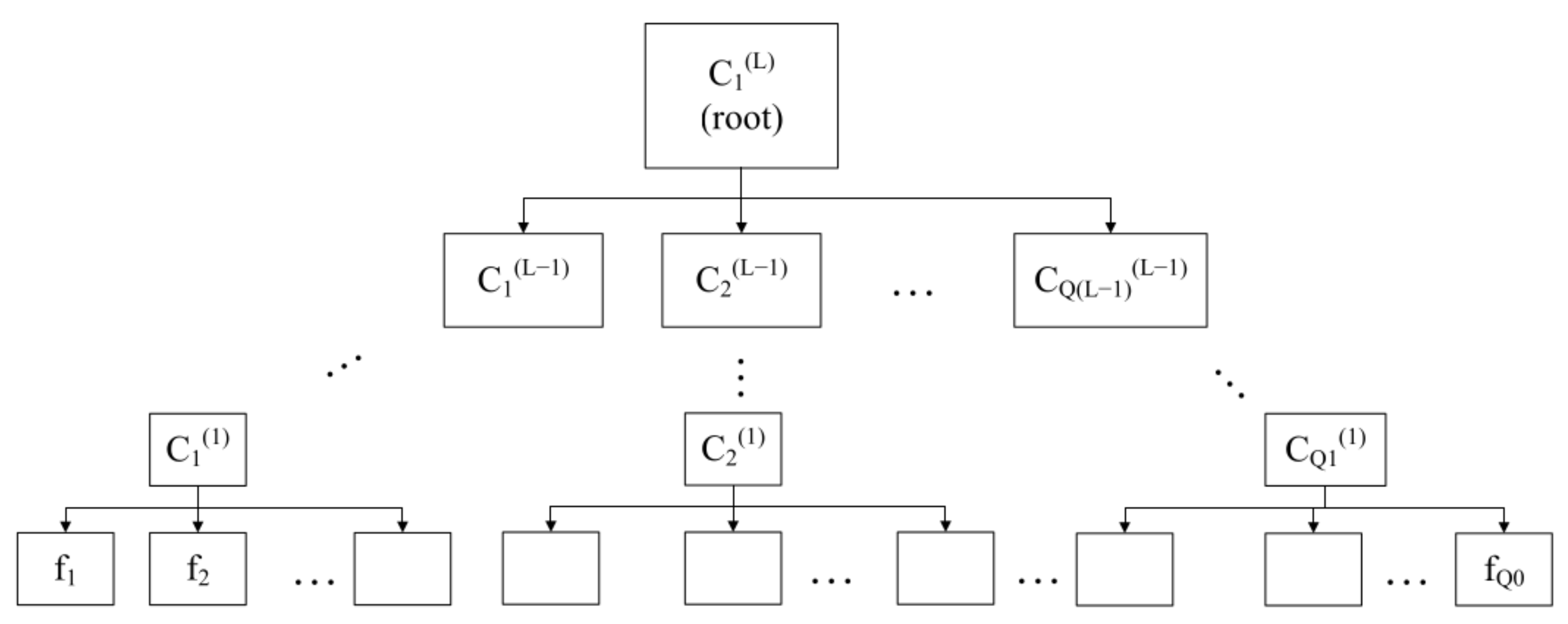
We analyzed nine indicators capturing the quality of healthcare systems in sixteen Polish voivodeships. The indicators were grouped under three main categories: inhabitants’ health improvement, financial management, and consumer satisfaction. We elicited the preferences in the form of marginal value functions for all inputs and outputs and weight constraints. We report the results given a comprehensive efficiency index encompassing all relevant viewpoints and the three subproblems that allow for an understanding of each voivodeship’s strong and weak points. The paper’s three significant contributions, along with their essential aspects, are summarized in Figure 1.

The paper’s remainder is organized as follows. Section 2 describes an additive value-based efficiency model. Section 3 defines a hierarchical structure of inputs and outputs, while Section 4 describes a respective framework for robustness analysis. In Section 5, we report the outcomes of a case study concerning the efficiency assessment of the healthcare system in Poland. The last section concludes the paper.

2. Additive Value-Based Efficiency Analysis

Let us consider a set of DMUs $\mathcal{D}=\{D_1,\dots ,D_K\}$. In value-based analysis, efficiency $E_o$ of $DM{U}_o\in \mathcal{D}$ is defined using an additive value model:

$$E_o=\sum _{q=1}^Q{w}_q·u_q(DM{U}_o),$$

(1)

where $w_q$ is the weight of factor q (i.e., input $x\in \mathit{x}=\{x_1,x_2,\dots ,x_m\}$ or output $y\in \mathit{y}=\{y_1,y_2,\dots ,y_n\}$), such that ${\sum }_{q=1}^Q{w}_q=1$, and $u_q$ is a monotonic marginal value function for q. It is nondecreasing for outputs and nonincreasing for inputs. To verify if $DM{U}_o$ is efficient, we solve the following Linear Programming (LP) model, minimizing the maximal distance of efficiency of $DM{U}_o$ to any other unit:

$$\mathrm{Minimize}{d}_o$$

s.t.

$$\begin{array}{c}\hfill \left.\begin{array}{c}\sum _{q=1}^Q{w}_q{u}_q(DM{U}_k)-\sum _{q=1}^Q{w}_q{u}_q(DM{U}_o)\le d_o, \mathrm{for} k=1,\dots ,K,\hfill \\ d_o\ge 0,\hfill \\ \sum _{q=1}^Q{w}_q=1,\hfill \\ w_q\ge 0,q=1,\dots ,Q,\hfill \\ \mathbf{w}\in S_w,\hfill \end{array}\right\}\end{array}$$

(2)

where $S_w$ is the feasible weight vector space delimited by the linear constraints. The optimal value of $d_o$, denoted by $d_o^{*}$, represents the minimal distance of $DM{U}_o$ from the efficient unit. If $d_o^{*}=0$, $DM{U}_o$ attains the greatest efficiency for at least one feasible weight vector, which implies that it is efficient. When $d_o^{*}>0$, for all feasible weights, there is at least one unit with an efficiency greater than $E_o$, denoting the lack of efficiency of $DM{U}_o$.

3. A Hierarchical Structure of Inputs and Outputs

The DMUs consume m inputs $\mathit{x}$ and produce n outputs $\mathit{y}$. To simplify the notation, we aggregate all inputs and outputs into a single set of factors $\mathit{f}=\mathit{x}\cup \mathit{y}=\{f_1,f_2,\dots ,f_{Q_0}\}$. Set $\mathit{f}$ forms level 0 of the hierarchy. These factors are grouped into $Q_1$ categories of the first level, named ${\mathit{C}}^{(\mathbf{1})}=\{c_1^{(1)},c_2^{(1)},\dots ,c_{Q_1}^{(1)}\}$. Analogously, the first-level categories can be grouped into second-level categories, forming a set ${\mathit{C}}^{(\mathbf{2})}=\{c_1^{(2)},c_2^{(2)},\dots ,c_{Q_2}^{(2)}\}$, etc. The entire structure contains L levels. In the last (L-th) level, there is only a single category ($c_1^{(L)}$), called a root.

From the mathematical viewpoint, the factors and categories form a tree (see Figure 2). The set of all nodes in the tree (factors and categories) is denoted by $\mathit{N}=f\cup C^{(1)}\cup C^{(2)}\cup \dots \cup C^{(L)}$. For each node $t\in \mathit{N}\backslash \left\{root\right\}$, we define its parent $p(t)$ as a category in which it is directly contained. The set of direct children of category $c_i^{(l)}$ is marked as $ch(c_i^{(l)})=\{t\in \mathit{N}$:$p(t)=c_i^{(l)}\}$. The set of indirect children of category $c_i^{(l)}$ contains all direct children of $c_i^{(l)}$ $(ch(c_i^{(l)}))$ and their direct and indirect children until reaching the tree’s leaves. For each category at hierarchy level $c_i^{(l)}$, we define set $A_{c_i^{(l)}}$ as a subset of $\mathit{f}$ (inputs and outputs), which are the indirect children of $c_i^{(l)}$. In particular, all factors are indirect children of the root category, i.e., $A_{c_1^{(L)}}=\mathit{f}$. On the contrary, for an elementary factor f, $A_f$ is a singleton, i.e., $A_f=\left\{f\right\},f\in \mathit{f}$. To maintain the spirit of DEA, for each category $c_i^{(l)}$, the respective set of factors ($A_{c_i^{(l)}}$) needs to contain at least one input and one output, i.e., $A_{c_i^{(l)}}\cap \mathit{x}\ne \varnothing$ and $A_{c_i^{(l)}}\cap \mathit{y}\ne \varnothing$, for $l=1,2,\dots ,L,i=1,2,\dots ,Q_l$.

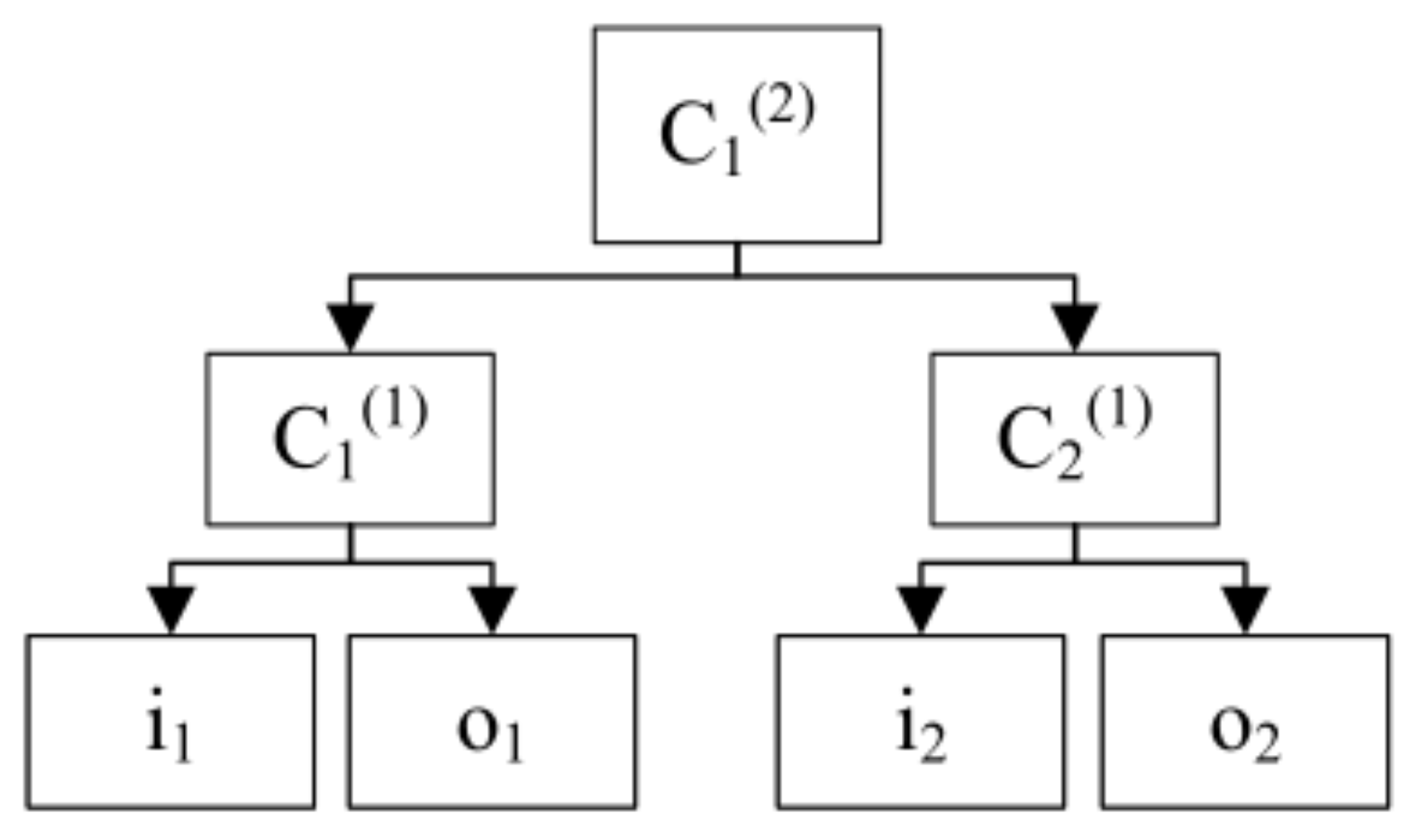
To illustrate the notation used in the paper, we will describe it using a simple hierarchy of factors in Figure 3. This example involves two inputs ($\mathit{x}=\{i_1,i_2\}$) and two outputs ($\mathit{y}=\{o_1,o_2\}$). The set of factors $\mathit{f}$ containing all elements from $\mathit{x}$ and $\mathit{y}$ is $\mathit{f}=\{i_1,o_1,i_2,o_2\}$. Overall, there are four factors ($Q_0=4$), two first-level categories (${\mathit{C}}_{\mathbf{1}}=\{C_1^{(1)},C_2^{(1)}\}$; $Q_1=2$), and one root corresponding to a second-level category (${\mathit{C}}_{\mathbf{2}}=\left\{C_1^{(2)}\right\}$; $Q_2=1$). The hierarchy contains two levels of categories ($L=2$). The parent category for input $i_1$ is $C_1^{(1)}$ ($p(i_1)=C_1^{(1)}$). For $C_1^{(1)}$ and $C_2^{(1)}$, the parent category is $C_1^{(2)}$, i.e., $p(C_1^{(1)})=p(C_2^{(1)})=C_1^{(2)}$. The considered sets of factors $A_{C_i^{(k)}}$ for example categories are the following: $A_{i_1}=\left\{i_1\right\}$, $A_{C_1^{(1)}}=\{i_1,o_1\}$, $A_{C_2^{(1)}}=\{i_2,o_2\}$, and $A_{C_1^{(2)}}=\mathit{f}=\{i_1,i_2,o_1,o_2\}$.

Given a hierarchy of relevant factors and categories, we assign weight $w_t$ to each node t except the root. Moreover, we admit specifying the linear constraints for these weights at each hierarchy level. Factors or categories involved in a single constraint must have a common parent. For example, for the considered hierarchy, the constraint can take the form $w_{i_1}\le 2·w_{o_1}$ or $w_{c_1^{(1)}}\ge w_{c_2^{(1)}}$, as $i_1$ and $o_1$ or $C_1^{(1)}$ and $C_2^{(1)}$ have the same parent. On the contrary, the example constraint $w_{i_1}\le w_{i_2}$ is not allowed, because $i_1$ and $i_2$ have different parents ($p(i_1)\ne p(i_2)$). The space of weight vectors that meet these restrictions is denoted by $S_w$.

To introduce weight restrictions, we consider additional variables (${\widehat{w}}_q$), representing the aggregated weights of elementary factors in the hierarchy. They are defined as the products of all weights on the path from the analyzed category ($c_i^{(l)}$) at the hierarchy level l to the analyzed factor f:

$${\widehat{w}}_q^{c_i^{(l)}}=w_q·\prod _{t=1,\dots ,l-1\wedge t\in c_i^{(l)}\wedge f\in A_t}{w}_t.$$

(3)

For factor $i_1$ in the considered example, when taking into account the root category ($C_1^{(2)}$), the above formula takes the following form ${\widehat{w}}_{i_1}^{C_1^{(2)}}=w_{i_1}·w_{C_1^{(1)}}$, and when considering category $C_1^{(1)}$, it is expressed as follows ${\widehat{w}}_{i_1}^{C_1^{(1)}}=w_{i_1}$.

We analyze the efficiency of $DM{U}_o$ in each node of the hierarchy. For category $c_i^{(l)}$, such efficiency is defined as follows:

$$E_o^{c_i^{(l)}}=\sum _{q\in A_{c_i^{(l)}}}{\widehat{w}}_q^{c_i^{(l)}}·u_q(DM{U}_o).$$

(4)

The true weights assigned to each hierarchy category $c_i^{(l)}$ from the set of the indirect children of the analyzed category $c_j^{(k)}$ are defined as the ratio of the sum of weights of indicators contained in this category and the sum of weights of indicators in the parent category:

$$w_{c_i^{(l)}}^{c_j^{(k)}}=\frac{{\sum }_{f\in A_{c_i^{(l)}}}{\widehat{w}}_f^{c_j^{(k)}}}{{\sum }_{f_p\in A_{p(c_i^{(l)})}}{\widehat{w}}_{f_p}^{c_j^{(k)}}}.$$

(5)

Note that the value of weight $w_{c_i^{(l)}}^{c_j^{(k)}}$ is always the same, regardless of the considered category ($c_j^{(k)}$), so we replace symbol $w_{c_i^{(l)}}^{c_j^{(k)}}$ with $w_{c_i^{(l)}}$. For example, when considering the root category ($C_1^{(2)}$), the weight $w_{i_1}$ of indicator $i_1$ in the considered example can be calculated as $w_{i_1}=\frac{{\widehat{w}}_{i_1}^{C_1^2}}{{\widehat{w}}_{i_1}^{C_1^2}+{\widehat{w}}_{o_1}^{C_1^2}}$, whereas the weight $w_{C_2^{(1)}}$ of category $C_2^{(1)}$ is $w_{C_2^{(1)}}=\frac{{\widehat{w}}_{i_2}^{C_1^{(2)}}+{\widehat{w}}_{o_2}^{C_1^{(2)}}}{{\widehat{w}}_{i_1}^{C_1^{(2)}}+{\widehat{w}}_{o_1}^{C_1^{(2)}}+{\widehat{w}}_{i_2}^{C_1^{(2)}}+{\widehat{w}}_{o_2}^{C_1^{(2)}}}$.

4. Robustness Analysis for Additive Value-Based Efficiency Analysis with a Hierarchical Structure of Factors

The standard value-based efficiency model verifies if each DMU is efficient. Such an analysis builds on the weight vector that is the most advantageous for a given DMU, allowing it to minimize the distance from some efficient DMU. In this section, we introduce a suite of methods that investigate the robustness of efficiency outcomes given all feasible weights. They can be divided into two groups. First, the exact approaches use mathematical programming to find the extreme outcomes for each DMU. In turn, the probabilistic methods estimate the stochastic acceptability indices based on Monte Carlo simulations, reflecting the distributions of possible results. Each group concerns three relevant viewpoints: distances to the efficient unit, ranks, and pairwise preference relations. In what follows, we present the approaches that are flexible enough to determine the relevant results in each hierarchy node.

4.1. Exact Methods

In this section, we present the mathematical programming models that determine the exact robust results. These include extreme (the most and the least advantageous), necessary (observable for all feasible weight vectors), and possible (holding for at least one feasible weight vector) conclusions. Let us first focus on verifying the stability of distances to the efficient unit. The best (minimal) distance $d_{*,o}^{c_i^{(l)}}$ for $DM{U}_o$ considering category $c_i^{(l)}$ can be computed by solving the following model:

$$\mathrm{Minimize}{d}_o^{c_i^{(l)}}$$

s.t.

$$\begin{array}{c}\hfill \left.\begin{array}{l}\sum _{q\in A_{c_i^{(l)}}}{\widehat{w}}_q^{c_i^{(l)}}{u}_q(DM{U}_k)-\sum _{q\in A_{c_i^{(l)}}}{\widehat{w}}_q^{c_i^{(l)}}{u}_q(DM{U}_o)\le d_o^{c_i^{(l)}}, \mathrm{for} k=1,\dots ,K,\hfill \\ d_o^{c_i^{(l)}}\ge 0,\hfill \\ \left.\begin{array}{c}\sum _{q\in A_{c_i^{(l)}}}{\widehat{w}}_q^{c_i^{(l)}}=1,\hfill \\ {\widehat{w}}_q\ge 0,q\in A_{c_i^{(l)}},\hfill \\ w_t=\frac{{\sum }_{f\in A_t}{\widehat{w}}_f^{c_i^{(l)}}}{{\sum }_{f\in A_{p(t)}}{\widehat{w}}_f^{c_i^{(l)}}}\in S_w,fort\in \mathit{N}\backslash \left\{root\right\}.\hfill \end{array}\right\}\mathcal{W}\hfill \end{array}\right\}\end{array}$$

(6)

Similarly to the standard efficiency analysis, $DM{U}_o$ with $d_{*,o}^{c_i^{(l)}}=0$ is deemed efficient, given category $c_i^{(l)}$, while $d_{*,o}^{c_i^{(l)}}>0$ implies inefficiency.

To compute the worst (maximal) distance $d_o^{*,c_i^{(l)}}$ for $DM{U}_o$, given category $c_i^{(l)}$, we solve the following Mixed-Integer Linear Programming (MILP) model:

$$\mathrm{Maximize}{d}_o^{c_i^{(l)}}$$

s.t.

$$\begin{array}{c}\hfill \left.\begin{array}{c}\sum _{q\in A_{c_i^{(l)}}}{\widehat{w}}_q^{c_i^{(l)}}{u}_q(DM{U}_k)-d_o^{c_i^{(l)}}\ge \sum _{q\in A_{c_i^{(l)}}}{\widehat{w}}_q^{c_i^{(l)}}{u}_q(DM{U}_o)-C(1-b_k), \mathrm{for} k=1,\dots ,K,\hfill \\ \sum _{k=1,...,K}{b}_k=1,\hfill \\ b_k\in \{0,1\}, \mathrm{for} k=1,2,\dots ,K,\hfill \\ d_o^{c_i^{(l)}}\ge 0,\hfill \\ \mathcal{W},\hfill \end{array}\right\}\end{array}$$

(7)

where C is a large positive constant. The above model uses binary variables $b_k$, $k=1,\dots ,K$, to ensure that $d_o^{c_i^{(l)}}$ is equal to the efficiency difference between $DM{U}_o$ and some $DM{U}_k$, $k=1,\dots ,K$, for which $b_k=1$. Maximizing $d_o^{c_i^{(l)}}$ guarantees that we obtain the greatest possible difference observable in the set of feasible weights $\mathcal{W}$. Note that when $b_k=0$, the respective constraint is satisfied for all possible variable values; hence, it is relaxed.

The second perspective concerns the bounds of efficiency ranks attained by $DM{U}_o$. To find the best (minimal) rank $R_{*,o}^{c_i^{(l)}}$ of $DM{U}_o$, given category $c_i^{(l)}$, we minimize the number of other DMUs with greater efficiencies than $E_o^{c_i^{(l)}}$:

$$\mathrm{Minimize}1+\sum _{k=1,...,K;k\ne o}{b}_k$$

s.t.

$$\begin{array}{c}\hfill \left.\begin{array}{c}\sum _{q\in A_{c_i^{(l)}}}{\widehat{w}}_q^{c_i^{(l)}}{u}_q(DM{U}_k)-\sum _{q\in A_{c_i^{(l)}}}{\widehat{w}}_q^{c_i^{(l)}}{u}_q(DM{U}_o)\le C{b}_k, \mathrm{for} k=1,\dots ,K;k\ne o,\hfill \\ b_k\in \{0,1\}, \mathrm{for} k=1,2,\dots ,K;k\ne o,\hfill \\ \mathcal{W}.\hfill \end{array}\right\}\end{array}$$

(8)

Note that when $b_k=0$, $k=1,\dots ,K$, the respective constraint ensures that $DM{U}_o$ is ranked not worse than $DM{U}_k$ since $E_k^{c_i^{(l)}}\le E_o^{c_i^{(l)}}$. When $b_k=1$, $DM{U}_k$ is ranked better than $DM{U}_o$, deteriorating its best rank by one.

To obtain the worst (maximal) rank $R_o^{*,c_i^{(l)}}$ for $DM{U}_o$, given category $c_i^{(l)}$, we maximize the number of DMUs with the efficiencies not worse than $E_o^{c_i^{(l)}}$:

$$\mathrm{Maximize}1+\sum _{k=1,...,K;k\ne o}{b}_k$$

s.t.

$$\begin{array}{c}\hfill \left.\begin{array}{c}\sum _{q\in A_{c_i^{(l)}}}{\widehat{w}}_q^{c_i^{(l)}}{u}_q(DM{U}_o)-\sum _{q\in A_{c_i^{(l)}}}{\widehat{w}}_q^{c_i^{(l)}}{u}_q(DM{U}_k)\le C(1-b_k), \mathrm{for} k=1,\dots ,K;k\ne o,\hfill \\ b_k\in \{0,1\}, \mathrm{for} k=1,2,\dots ,K;k\ne o,\hfill \\ \mathcal{W}.\hfill \end{array}\right\}\end{array}$$

(9)

Note that when $b_k=1$, $k=1,\dots ,K$, the respective constraint ensures that $DM{U}_k$ is ranked no worse than $DM{U}_o$ since $E_o^{c_i^{(l)}}\le E_k^{c_i^{(l)}}$. This deteriorates the worst rank of $DM{U}_o$ by one. When $b_k=0$, the respective constraint is satisfied for all variable values; hence, it relaxed.

The third perspective focuses on the pairwise comparisons between DMUs using two relations: necessary and possible. Given the uncertainty of selecting a specific weight vector, the necessary relation can be considered robust. Specifically, $DM{U}_o$ is necessarily preferred to $DM{U}_k$, given category $c_i^{(l)}$ ($DM{U}_o{\succsim }_E^{N,c_i^{(l)}}DM{U}_k$), when $DM{U}_o$ is not worse at level $c_i^{(l)}$ in terms of efficiency than $DM{U}_k$ for all feasible weight vectors. Its truth for pair $(DM{U}_o,DM{U}_k)$ and category $c_i^{(l)}$ can be verified using the following model:

$$\mathrm{Minimize}{d}_{o,k}^{c_i^{(l)}},s.t.\sum _{q\in A_{c_i^{(l)}}}{\widehat{w}}_q^{c_i^{(l)}}{u}_q(DM{U}_o)-\sum _{q\in A_{c_i^{(l)}}}{\widehat{w}}_q^{c_i^{(l)}}{u}_q(DM{U}_k)\le d_{o,k}^{c_i^{(l)}} \mathrm{and} \mathcal{W}.$$

(10)

Its optimal solution $d_{o,k,*}^{c_i^{(l)}}$ is equal to the minimal difference between efficiencies of $DM{U}_o$ and $DM{U}_k$ observable in the set of feasible weights $\mathcal{W}$, given category $c_i^{(l)}$. If $d_{o,k,*}^{c_i^{(l)}}\ge 0$, then for all feasible weights $E_o^{c_i^{(l)}}\ge E_k^{c_i^{(l)}}$, and hence $DM{U}_o{\succsim }_E^{N,c_i^{(l)}}DM{U}_k$. Otherwise, $\neg (DM{U}_o{\succsim }_E^{N,c_i^{(l)}}DM{U}_k)$ because there is at least one feasible weight vector, such that $E_o^{c_i^{(l)}}<E_k^{c_i^{(l)}}$.

Furthermore, $DM{U}_o$ is possibly preferred to $DM{U}_k$, given category $c_i^{(l)}$ ($DM{U}_o{\succsim }_E^{P,c_i^{(l)}}DM{U}_k$), when $DM{U}_o$ is not worse at level $c_i^{(l)}$ in terms of efficiency than $DM{U}_k$ for at least one feasible weight vector. Its truth for pair $(DM{U}_o,DM{U}_k)$ and category $c_i^{(l)}$ is verified using the following model:

$$\mathrm{Maximize}{d}_{o,k}^{c_i^{(l)}},s.t.\sum _{q\in A_{c_i^{(l)}}}{\widehat{w}}_q^{c_i^{(l)}}{u}_q(DM{U}_o)-\sum _{q\in A_{c_i^{(l)}}}{\widehat{w}}_q{u}_q^{c_i^{(l)}}(DM{U}_k)\ge d_{o,k}^{c_i^{(l)}} \mathrm{and} \mathcal{W}.$$

(11)

Its optimal solution $d_{o,,k}^{c_i^{(l)},*}$ is equal to the maximal difference between efficiencies of $DM{U}_o$ and $DM{U}_k$ observable in the set of feasible weights $\mathcal{W}$, given category $c_i^{(l)}$. If $d_{o,k}^{c_i^{(l)},*}\ge 0$, then for at least one feasible weight $E_o^{c_i^{(l)}}\ge E_k^{c_i^{(l)}}$, and hence, $DM{U}_o{\succsim }_E^{P,c_i^{(l)}}DM{U}_k$. Otherwise, $\neg (DM{U}_o{\succsim }_E^{P,c_i^{(l)}}DM{U}_k)$ because there is no feasible weight vector, such that $E_o^{c_i^{(l)}}\ge E_k^{c_i^{(l)}}$.

The relevant properties of the exact robust results given the hierarchical structure are presented in Appendix A. The formulations of example mathematical programming models that support understanding the general formulations are given in Appendix B.

4.2. Simulation-Based Methods

The results determined with mathematical programming are often insufficiently conclusive. In particular, the difference between extreme distances or ranks may be significant, the necessary relation may be poor, and the possible relation may be very rich. If so, it would be helpful to determine the distribution of results observed for the set of feasible weight vectors. Unfortunately, such distribution cannot be computed exactly. However, using Monte Carlo simulations, we can estimate the share of feasible weight space confirming a particular outcome. Specifically, we use the hit-And-run algorithm to generate a predefined number of weight vector samples [27]. We generate weights for all categories and factors while respecting that the sum of weights of categories or factors with the same parent must be equal to one. In the example problem, the sum of the weights of two categories $C_1^{(1)}$ and $C_2^{(1)}$ must be equal to one ($w_{C_1^{(1)}}+w_{C_2^{(1)}}=1)$, and the sums of weights assigned to the elementary indicators in the same category also need to be one ($w_{i_1}+w_{o_1}=1$ and $w_{i_2}+w_{o_2}=1$). Moreover, we obey the provided weight constraints for all hierarchy levels. After generating a predefined number of weight samples, we compute the efficiencies of all DMUs for each. This lets us calculate the relevant stochastic acceptability indices estimating the respective shares of feasible weight vectors.

In what follows, when considering category $c_i^{(l)}$ and referring to weight vectors, we mean the weights assigned to all categories and factors that are direct or indirect children of $c_i^{(l)}$ in the hierarchy. The most interesting stochastic acceptabilities are defined as follows:

• Distance Acceptability Interval Index ($DAI{I}^{c_i^{(l)}}(DM{U}_o,b_i)$) for unit $DM{U}_o$, interval $b_i\subseteq [0,1]$, and category $c_i^{(l)}$ is the share of feasible weight vectors for which $E_o^{c_i^{(l)}}$ belongs to $b_i$. Note that all intervals must be disjoint ($b_i\cap b_j=\varnothing ,i\ne j$), and their sum must cover the space of possible distances ($b_1\cup b_2\cup \dots \cup b_z=[0,1]$; z—the number of intervals).
• Efficiency Rank Acceptability Index ($ERA{I}^{c_i^{(l)}}(DM{U}_o,r)$) for unit $DM{U}_o$ and rank r is the share of feasible weight vectors for which $DM{U}_o$ attains r-th position in the efficiency ranking of all DMUs given category $c_i^{(l)}$.
• Pairwise Efficiency Outranking Index ($PEO{I}^{c_i^{(l)}}(DM{U}_o,DM{U}_k)$) for pair $(DM{U}_o$, $DM{U}_k)$ and category $c_i^{(l)}$ is the share of feasible weight vectors for which $DM{U}_o$ is at least as efficiency as $DM{U}_k$ at level $c_i^{(l)}$, i.e., $E_o^{c_i^{(l)}}\ge E_k^{c_i^{(l)}}$.

Moreover, we compute the expected distance $Ed$ to the efficient unit and expected rank $ER$ for each DMU [28]. This is performed by averaging the distances or ranks observed for all samples. Note that by default, we use uniform distribution for weight sampling. However, the weights can be generated from any predefined distribution, but it is hard to define as it requires in-depth knowledge about the specific application domain.

In Appendix C, we illustrate the process of computing the stochastic results on a small sample of weight vectors.

5. Case Study concerning Evaluation of Healthcare System in Poland

This section reports the results of a case study concerning an assessment of the quality of the healthcare system in Poland. This sector faces the challenge of improving the quality of provided services. This can be attained by advancing some indicators reflecting both the system’s functioning and the perception by patients. We consider sixteen voivodeships (provinces) in Poland as DMUs (see

Table 1. Values of inputs and outputs related to the healthcare systems in sixteen Polish voivodeships [29] (data publicly available at https://www.pwc.pl/pl/publikacje/2019/indeks-sprawnosci-ochrony-zdrowia-2018.html, accessed on 22 May 2023).

Voivodeship	Short Name	${\mathit{H}}_1$	${\mathit{H}}_2$	${\mathit{H}}_3$	${\mathit{F}}_1$	${\mathit{F}}_2$	${\mathit{F}}_3$	${\mathit{S}}_1$	${\mathit{S}}_2$	${\mathit{S}}_3$
Zachodniopomorskie	ZPM	44.44	4.05	17.6	−1.5	46.1	46.9	19.23	3.55	9.30
Pomorskie	POM	45.31	5.36	21.3	0.08	38.9	51.3	27.04	3.82	33.33
Warmińsko−Mazurskie	WM	43.34	7.11	15.7	−1.09	44.8	47.8	22.19	3.72	22.73
Podlaskie	PDL	37.54	6.93	15.8	2.3	49.4	43.4	19.47	3.61	11.11
Lubuskie	LBU	50.21	5.83	18.0	1.9	42.0	51.3	18.32	3.84	13.04
Wielkopolskie	WLKP	47.88	4.36	25.7	−0.3	43.4	50.5	15.16	3.69	17.24
Kujawsko−Pomorskie	KP	39.90	6.80	15.7	3.8	46.5	41.8	22.36	3.77	33.33
Mazowieckie	MAZ	38.59	5.32	16.7	−1.57	47.4	47.8	20.26	3.62	20.56
Lubelskie	LBL	45.17	6.74	8.1	0.41	51.8	43.0	13.40	3.77	20.37
Dolnośląskie	DSL	45.04	7.66	13.8	−1.77	50.8	43.8	24.55	3.57	17.28
Opolskie	OPO	33.71	6.88	10.0	−0.36	44.1	40.9	23.03	3.67	35.71
Łódzkie	LDZ	42.00	5.88	6.0	1.02	50.6	47.3	19.90	3.78	15.15
Śląskie	SL	40.70	4.54	13.9	−1.63	55.5	39.1	22.02	3.75	16.88
Świętokrzyskie	SW	41.14	5.79	7.8	0.17	49.5	47.2	12.44	3.57	29.17
Małopolskie	MLP	32.22	5.61	9.1	0.79	43.7	44.3	18.27	3.64	25.84
Podkarpackie	PKR	38.73	5.76	1.9	−4.31	48.0	45.8	14.39	3.84	20.51

). These administrative areas govern their healthcare independently, so it makes sense to highlight their differences using a uniformly computed set of indicators. Such an evaluation is critical, given the rapid development of new technologies and major transformations in the healthcare sector.

Following [29], we consider three main categories of factors representing desirable characteristics in the complex healthcare system. Two areas—health improvement and financial management—are based on objective indicators and parameters, whereas the system’s evaluation by patients is, to some extent, subjective. In particular, improving health is the ultimate aim of the healthcare system. In this regard, it is relevant to consider the example dimensions of the health status that are affected by how the system is operated, given the ever-growing needs of patients. Financial management is essential in healthcare, as this sector experiences the availability of limited resources. Hence, it is vital to assess the financial situation of medical facilities, the management of infrastructure, and the economic efficiency of treatments and therapies. Finally, consumer satisfaction is becoming more and more important in evaluating the healthcare sector. Thus, it is desirable to consider the quality of services, comfort in using patients’ services, and patient rights.

The hierarchy of inputs and outputs for the case study is presented in Figure 4. Among the nine factors, there are six outputs ($H_1$, $H_3$, $F_1$, $F_3$, $S_2$, and $S_3$) and three inputs ($H_2$, $F_2$, and $S_1$). The selected indicators are representative of the three dimensions and the viewpoints of the most important stakeholders. The indicators in the health improvement category (H) are representative of the dimensions of preventing diseases ($H_1$), their exacerbation ($H_2$), and deaths ($H_3$). The factors considered in the financial management category stand for the financial situation of healthcare units ($F_1$) and infrastructure management ($F_2$ and $F_3$). The inputs and outputs in the system’s evaluation category (S) represent the waiting time ($S_1$), official quality system ($S_2$), and patient satisfaction ($S_3$). Moreover, we verified that the trends that these indicators confirm also represent other factors that could be considered in the three categories. Note that analysis including over 40 indicators available for assessing the healthcare system in Poland [29] would not make much sense in the context of DEA, as the number of inputs and outputs would be too large compared to the number of DMUs. Typically, such analyses indicate that all or almost all units are efficient, as even the worst performers tend to specialize in some particular aspects. Hence, we opted for an analysis with a reduced—though carefully selected—set of indicators. The performances of the sixteen voivodeships in terms of nine considered factors are given in Table 1.

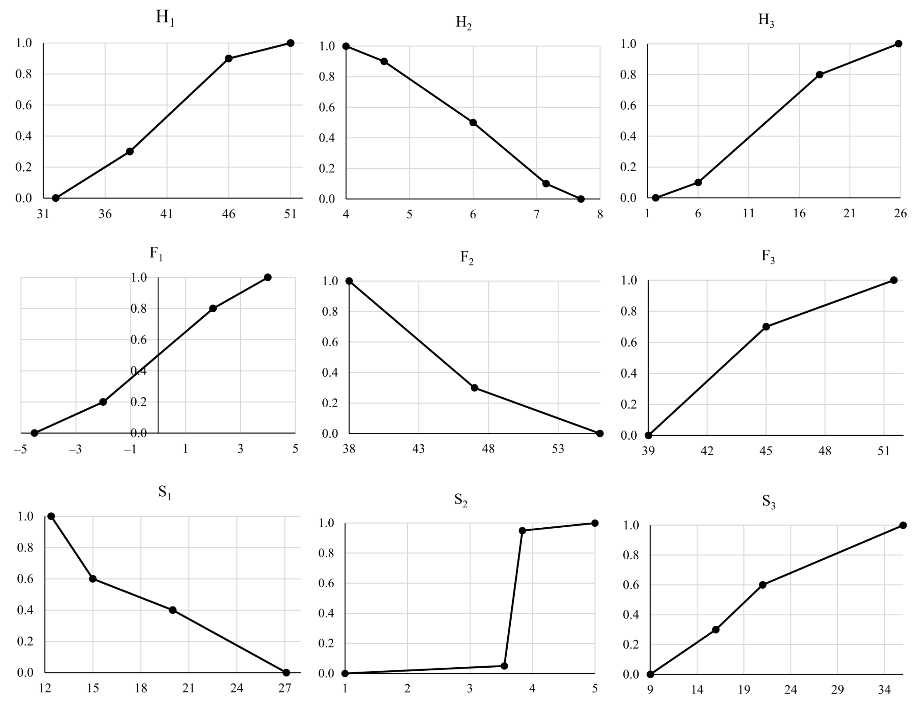
For all factors, we elicited marginal value functions from experts in the healthcare system in Poland. They are provided in Figure 5. They are decreasing for inputs and increasing for outputs. Moreover, they differ in shape. The function is, e.g., close to linear for $H_2$, convex for $F_3$, concave for $F_2$, and S-shaped for $S_2$. Moreover, we incorporated the relative and absolute weight constraints. The category of inhabitants’ health improvement is more important than the two other categories. Hence, we introduced the following constraints: $w_H\ge w_F$ and $w_H\ge w_S$, where $w_H$, $w_F$, and $w_S$ are the weights of the three categories. Finally, we wanted to avoid both the minor and dominating roles of any individual factor or category in the analysis. Hence, we restricted the weight of each category to be not less than $0.2$ and the weights of second-level elementary factors to the interval $[0.2,0.5]$. In what follows, we discuss the results attained in the root hierarchy level and for each of the three categories separately.

5.1. Comprehensive Evaluation of the Quality of Healthcare Systems

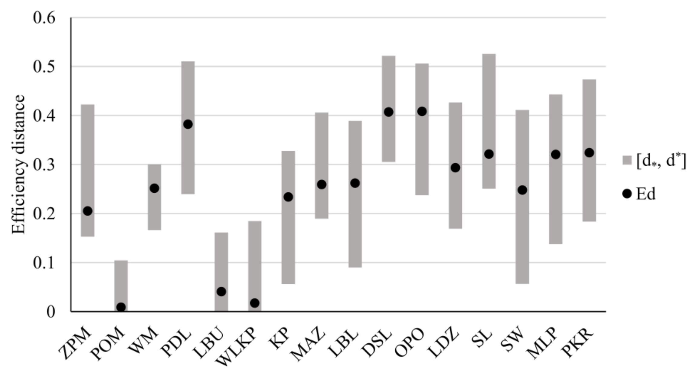
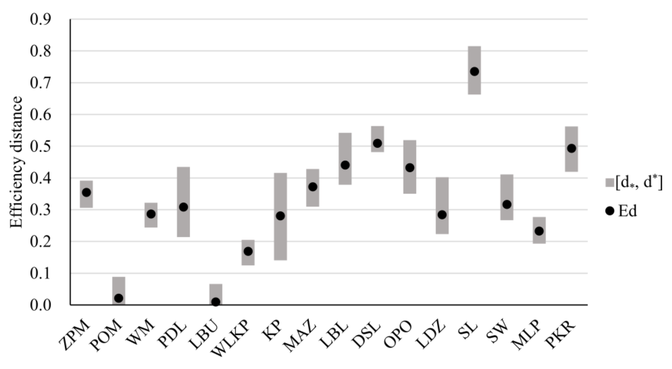
In this section, we discuss the results of the comprehensive assessment of Polish voivodeships, taking into account all nine indicators. Figure 6 presents the extreme and expected distances to the best unit for each analyzed province. Three voivodeships are efficient: POM, LBU, and WLKP. POM also attains the lowest maximal distance ($0.105$), which confirms its most favorable evaluation of the healthcare system for all feasible weights. Moreover, the distances for POM are the most stable, as it is characterized by the narrowest range ($d^{I,*}-d_{*}^I=0.105$). Among the efficient provinces, WLKP has the worst pessimistic distance to the best province. However, its expected distance is better than that of LBU, meaning that for some weight vectors, WLKP performs worse than LBU, but its efficiency score is closer to the best province on average. The worst provinces in the most and the least favorable scenarios are DSL ($d_{*}^I=0.306$, $d^{I,*}=0.522$) and SL ($d_{*}^I=0.251$, $d^{I,*}=0.526$). The greatest sensitivity of the distances depending on the selected weight vector is observed for SW, as the width of its distance interval equals $0.355$.

The analysis of extreme distances can be enriched with the distribution of distances over all feasible weight vectors (see

Table 2. Distribution of distances to the best unit for Polish voivodeships in the comprehensive analysis of the healthcare system.

DAII	[0.0, 0.1]	(0.1, 0.2]	(0.2, 0.3]	(0.3, 0.4]	(0.4, 0.5]	(0.5, 0.6]	(0.6, 0.7]	(0.7, 0.8]	(0.8, 0.9]	(0.9, 1.0]
ZPM	0	0.523	0.475	0.002	0	0	0	0	0	0
POM	1	0	0	0	0	0	0	0	0	0
WM	0	0.006	0.956	0.038	0	0	0	0	0	0
PDL	0	0	0.006	0.714	0.280	0	0	0	0	0
LBU	0.992	0.008	0	0	0	0	0	0	0	0
WLKP	1	0	0	0	0	0	0	0	0	0
KP	0	0.160	0.798	0.042	0	0	0	0	0	0
MAZ	0	0.001	0.963	0.036	0	0	0	0	0	0
LBL	0	0.074	0.729	0.197	0	0	0	0	0	0
DSL	0	0	0	0.406	0.594	0	0	0	0	0
OPO	0	0	0	0.407	0.587	0.006	0	0	0	0
LDZ	0	0	0.599	0.401	0	0	0	0	0	0
SL	0	0	0.254	0.732	0.014	0	0	0	0	0
SW	0	0.127	0.762	0.111	0	0	0	0	0	0
MLP	0	0	0.307	0.675	0.018	0	0	0	0	0
PKR	0	0.002	0.295	0.659	0.044	0	0	0	0	0

). The efficient provinces (POM, LBU, and WLKP) are the only ones whose distances were not greater than $0.1$ for some samples. When considering these three voivodeships, only for LBU, the distance was greater than $0.1$ for some marginal share of weights ($0.8\%$). Hence, these provinces are robustly better than the remaining ones. Among the inefficient units, the most favorable results were attained by ZPM and KP.

Some provinces are characterized by rather stable distance values. For example, for MAZ and WM, for over $95\%$ of weight vectors, the distance is the interval $(0.2,0.3]$. On the contrary, the distance for PKR varies more depending on the chosen weight vector. In this case, positive $DAII$s were observed for all buckets between $0.1$ and $0.5$ with the greatest values for the intervals $(0.3,0.4]$ ($DAII(PKR,(0.3,0.4])=65.9\%$) and $[0.2,0.3]$ ($DAII(PKR,(0.2,0.3])=29.5\%$). The complete ranking determined by the expected distances (see Figure 6) indicates POM ($0.009$) and WLKP ($0.017$) as the best units and DSL ($0.408$) and OPO ($0.409$) as the worst.

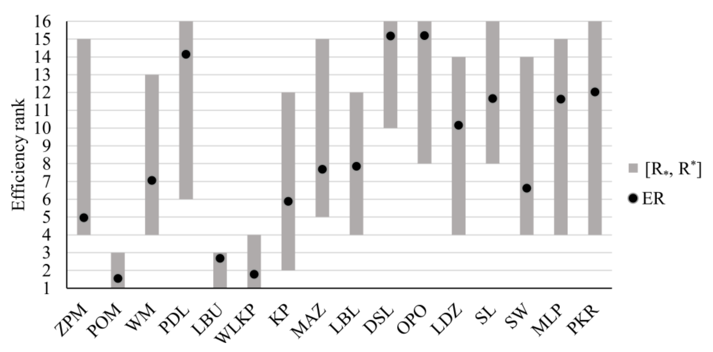
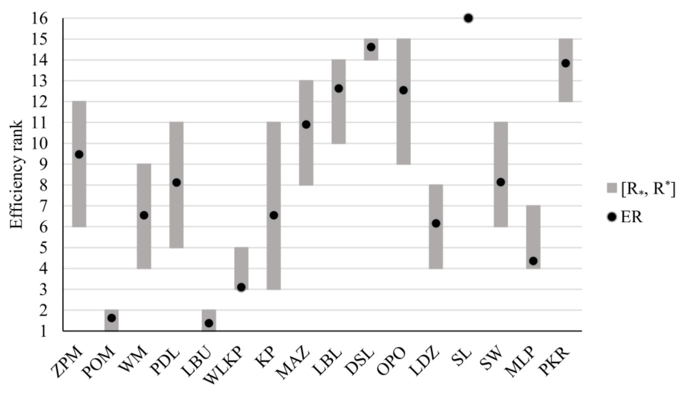
The results of robustness analysis for efficiency ranks are presented in Figure 7 and

Table 3. Distribution of ranks for Polish voivodeships in the comprehensive analysis of the healthcare system.

ERAI	1	2	3	4	5	6	7	8	9	10	11	12	13	14	15	16
ZPM	0	0	0	0.594	0.144	0.095	0.072	0.065	0.028	0.002	0	0	0	0	0	0
POM	0.577	0.303	0.120	0	0	0	0	0	0	0	0	0	0	0	0	0
WM	0	0	0	0.029	0.192	0.210	0.191	0.183	0.103	0.042	0.030	0.020	0	0	0	0
PDL	0	0	0	0	0	0	0	0	0	0.002	0.009	0.072	0.114	0.443	0.288	0.072
LBU	0.050	0.226	0.724	0	0	0	0	0	0	0	0	0	0	0	0	0
WLKP	0.373	0.471	0.156	0	0	0	0	0	0	0	0	0	0	0	0	0
KP	0	0	0	0.248	0.245	0.174	0.162	0.099	0.039	0.023	0.010	0	0	0	0	0
MAZ	0	0	0	0	0.101	0.161	0.215	0.171	0.220	0.096	0.033	0.003	0	0	0	0
LBL	0	0	0	0.033	0.084	0.151	0.149	0.158	0.256	0.104	0.044	0.017	0.004	0	0	0
DSL	0	0	0	0	0	0	0	0	0	0	0.003	0.022	0.042	0.140	0.325	0.468
OPO	0	0	0	0	0	0	0	0	0	0	0.001	0.001	0.017	0.217	0.311	0.453
LDZ	0	0	0	0	0	0.007	0.028	0.069	0.139	0.360	0.278	0.090	0.027	0.002	0	0
SL	0	0	0	0	0.007	0.010	0.028	0.032	0.041	0.120	0.150	0.184	0.335	0.068	0.022	0.003
SW	0	0	0	0.096	0.227	0.190	0.146	0.195	0.098	0.040	0.008	0	0	0	0	0
MLP	0	0	0	0	0	0	0.003	0.018	0.052	0.117	0.248	0.266	0.254	0.033	0.009	0
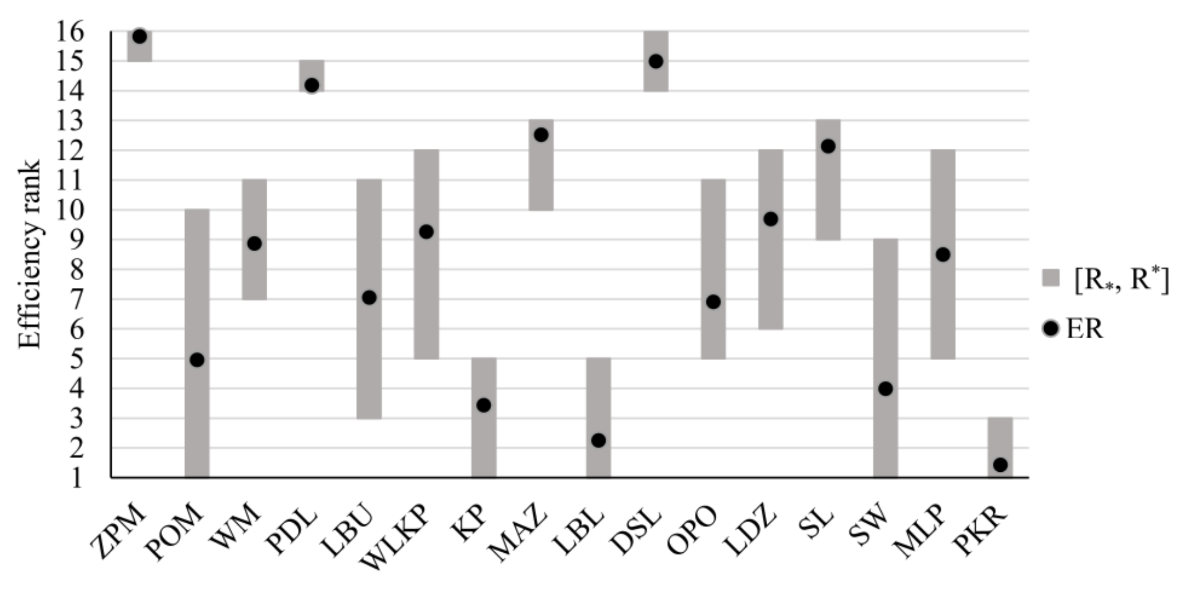
PKR	0	0	0	0	0	0.002	0.006	0.010	0.024	0.094	0.186	0.325	0.207	0.097	0.045	0.004

. The three efficient voivodeships attain the first rank in the most favorable scenario. POM and LBU are ranked third in their worst scenario, while WLKP falls fourth in the pessimistic case. These units are also the best, given their expected ranks. In this regard, POM ($1.543$) is followed by WLKP ($1.783$) and LBU ($2.674$). Among the inefficient units, KP is the most advantageous when considering the most favorable ranks ($R_{*}=2$). Other inefficient units ranked relatively high in their best scenario are ZPM, WM, LBL, LDZ, SW, MLP, and PKR ($R_{*}=4$). However, all inefficient provinces are ranked low in the least favorable scenario. The best maximal rank among them is observed for KP and LBL ($R^{*}=12$), while five provinces can be ranked at the bottom (PDL, DSL, OPO, SL, and PKR). Finally, the best expected ranks among inefficient units are attained by ZPM ($4.962$), KP ($5.878$), and SW ($6.611$), while the worst expected positions are associated with DSL ($15.166$) and OPO ($15.195$).

The analysis of efficiency rank acceptability indices (see Table 3) confirms the superiority of POM over other provinces. It is ranked first for most feasible weight vectors ($57.7\%$), and it is in the top two for almost $90\%$ of samples. Similarly, WLKP is at least second for over $84\%$ of samples, though its most frequent position is second rather than first. In turn, LBU is ranked third for most scenarios ($72.4\%$). Even though the best possible rank for KP is second, such a position was not observed for any weight vector. The highest for which ERAI for KP is positive is fourth ($24.8\%$). However, this place is predominantly occupied by ZPM, which is ranked in the interval $[4,7]$ for over $90\%$ of feasible scenarios.

Table 4. The necessary (N) and possible (P) efficiency preference relations for pairs of Polish voivodeships in the comprehensive analysis of the healthcare system.

Voivodeship	ZPM	POM	WM	PDL	LBU	WLKP	KP	MAZ	LBL	DSL	OPO	LDZ	SL	SW	MLP	PKR
ZPM	N		P	P			P	P	P	N	P	P	P	P	P	P
POM	N	N	N	N	P	P	N	N	N	N	N	N	N	N	N	N
WM	P		N	P			P	P	P	N	N	P	P	P	P	P
PDL	P		P	N				P	P	P	P	P	P	P	P	P
LBU	N	P	N	N	N	P	P	N	N	N	N	N	N	N	N	N
WLKP	N	P	N	N	P	N	P	N	N	N	N	N	N	N	N	N
KP	P		P	N	P	P	N	P	P	N	N	P	N	P	P	P
MAZ	P		P	P			P	N	P	P	P	P	P	P	P	P
LBL	P		P	P			P	P	N	N	P	P	N	P	P	P
DSL				P				P		N	P	P	P		P	P
OPO	P			P				P	P	P	N	P	P	P	P	P
LDZ	P		P	P			P	P	P	P	P	N	P	P	P	P
SL	P		P	P				P		P	P	P	N	P	P	P
SW	P		P	P			P	P	P	N	P	P	P	N	P	P
MLP	P		P	P			P	P	P	P	P	P	P	P	N	P
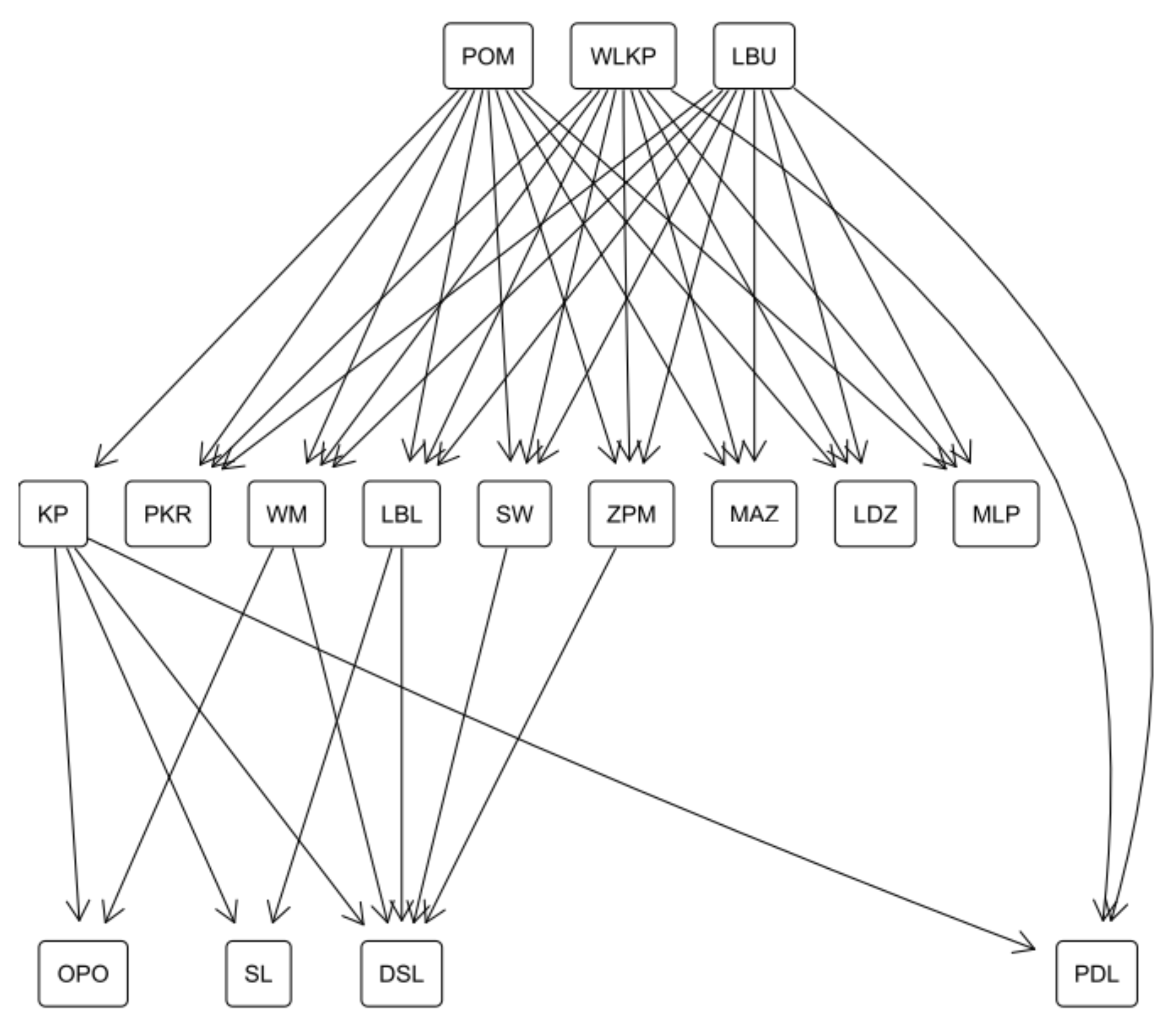
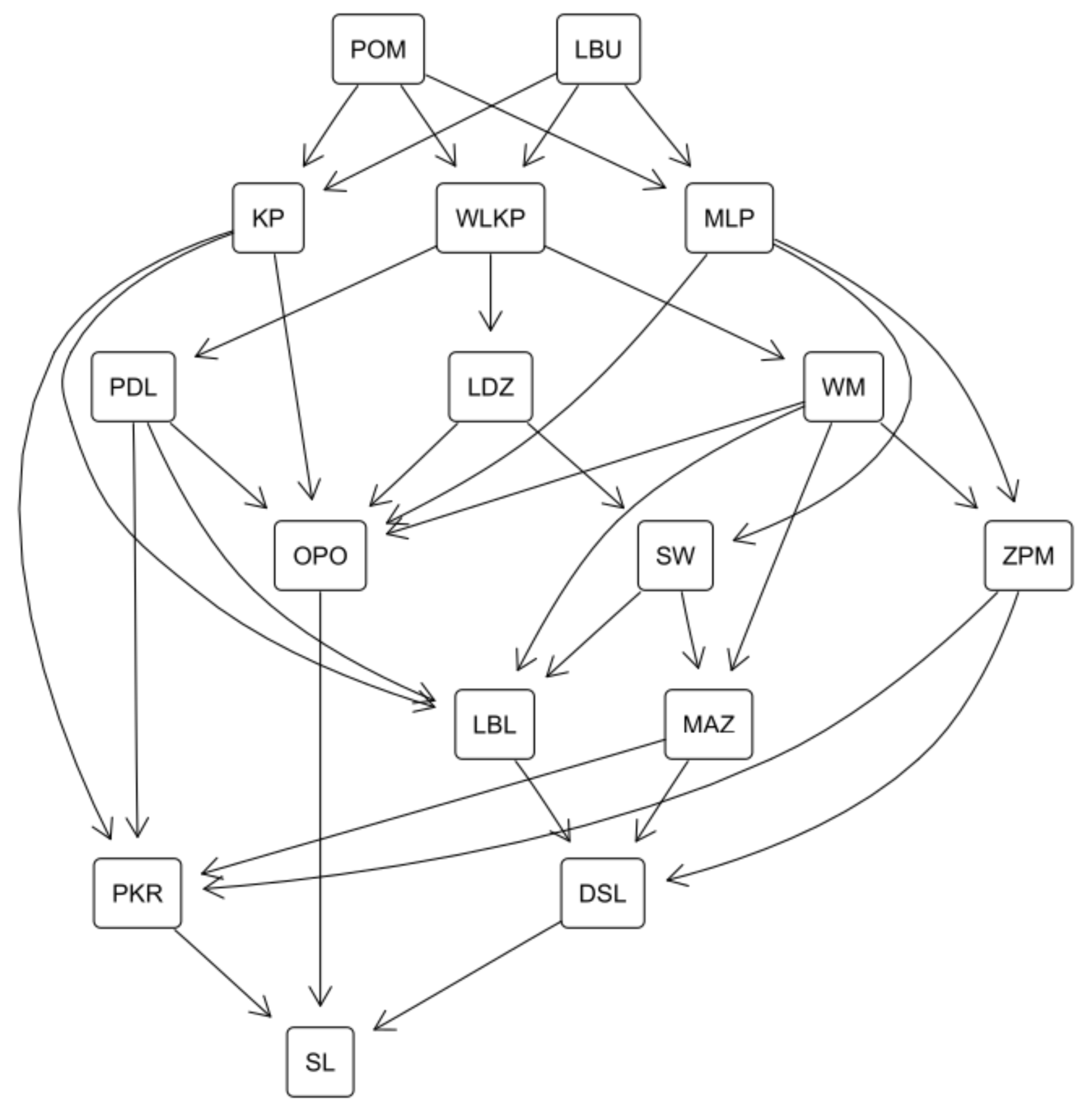
PKR	P		P	P			P	P	P	P	P	P	P	P	P	N

presents the results of exact robustness analysis from the perspective of pairwise comparisons. For clarity of presentation, the necessary relation is also presented in the form of the Hasse diagram in Figure 8. For efficient provinces (POM, WLKP, and LBU), no other unit is necessarily preferred to them. As expected, these provinces are necessarily preferred to the greatest number of other units. POM is robustly better than all thirteen inefficient provinces, and WLKP and LBU prove their superiority over all units but KP. Among the inefficient provinces, KP is necessarily preferred to the highest number (4) of other provinces. Eight voivodeships are not robustly as good as any other unit. The least favorable among them is DSL, which is not even possibly preferred to eight other provinces.

For pairs of voivodeships that are not related by the necessary preference, it is worth analyzing the pairwise efficiency outranking indices (see

Table 5. Pairwise efficiency outranking indices for pairs of Polish voivodeships in the comprehensive analysis of the healthcare system.

PEOI	ZPM	POM	WM	PDL	LBU	WLKP	KP	MAZ	LBL	DSL	OPO	LDZ	SL	SW	MLP	PKR
ZPM	1	0	0.835	1	0	0	0.690	0.962	0.852	1	1	0.989	1	0.791	1	0.994
POM	1	1	1	1	0.870	0.625	1	1	1	1	1	1	1	1	1	1
WM	0.165	0	1	1	0	0	0.286	0.609	0.630	1	1	0.890	0.918	0.481	0.960	0.967
PDL	0	0	0	1	0	0	0	0	0	0.760	0.748	0.006	0.095	0	0.039	0.146
LBU	1	0.130	1	1	1	0.181	1	1	1	1	1	1	1	1	1	1
WLKP	1	0.375	1	1	0.819	1	1	1	1	1	1	1	1	1	1	1
KP	0.310	0	0.714	1	0	0	1	0.758	0.805	1	1	0.953	0.974	0.651	0.996	0.990
MAZ	0.038	0	0.391	1	0	0	0.242	1	0.534	1	1	0.850	0.981	0.378	0.993	0.958
LBL	0.148	0	0.370	1	0	0	0.195	0.466	1	1	1	0.879	0.909	0.295	0.898	0.988
DSL	0	0	0	0.240	0	0	0	0	0	1	0.487	0.001	0.016	0	0.052	0.061
OPO	0	0	0	0.252	0	0	0	0	0	0.513	1	0.002	0.023	0	0	0.020
LDZ	0.011	0	0.110	0.994	0	0	0.047	0.150	0.121	0.999	0.998	1	0.745	0.051	0.757	0.849
SL	0	0	0.082	0.905	0	0	0.026	0.019	0.091	0.984	0.977	0.255	1	0.049	0.489	0.524
SW	0.209	0	0.519	1	0	0	0.349	0.622	0.705	1	1	0.949	0.951	1	0.997	0.992
MLP	0	0	0.040	0.961	0	0	0.004	0.007	0.102	0.948	1	0.243	0.511	0.003	1	0.568
PKR	0.006	0	0.033	0.854	0	0	0.010	0.042	0.012	0.939	0.980	0.151	0.476	0.008	0.432	1

). For some, one province proves better for most scenarios (see, e.g., ZPM and PKR with $PEO{I}^I(ZPM,PKR)=99.4\%$ or MAZ and MLP with $PEO{I}^I(MAZ,MLP)=99.3\%$). For other pairs, the shares of feasible scenarios confirming the preference in both directions are more balanced (see, e.g., MAZ and LBL with $PEO{I}^I(MAZ,LBL)=53.4\%$ and $PEO{I}^I(LBL,MAZ)=46.6\%$, or PKR and SL with $PEO{I}^I(PKR,SL)=47.6\%$ and $PEO{I}^L(SL,PKR)=52.4\%$).

5.2. The Category of Inhabitants’ Health Improvement

In this section, we focus on the results attained when considering only inputs and outputs from the inhabitants’ health improvement category. In addition, we emphasize the differences with respect to the comprehensive level.

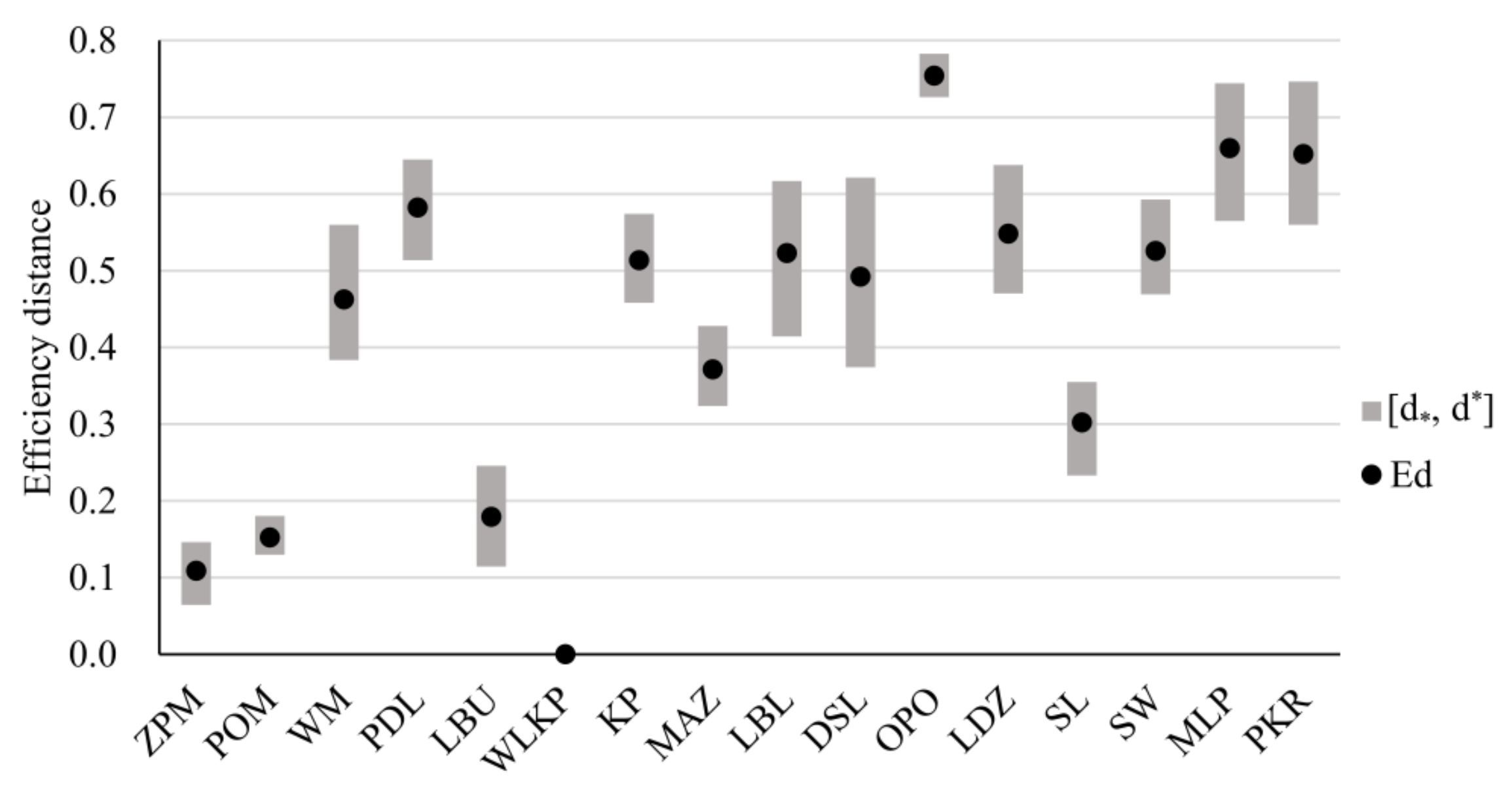
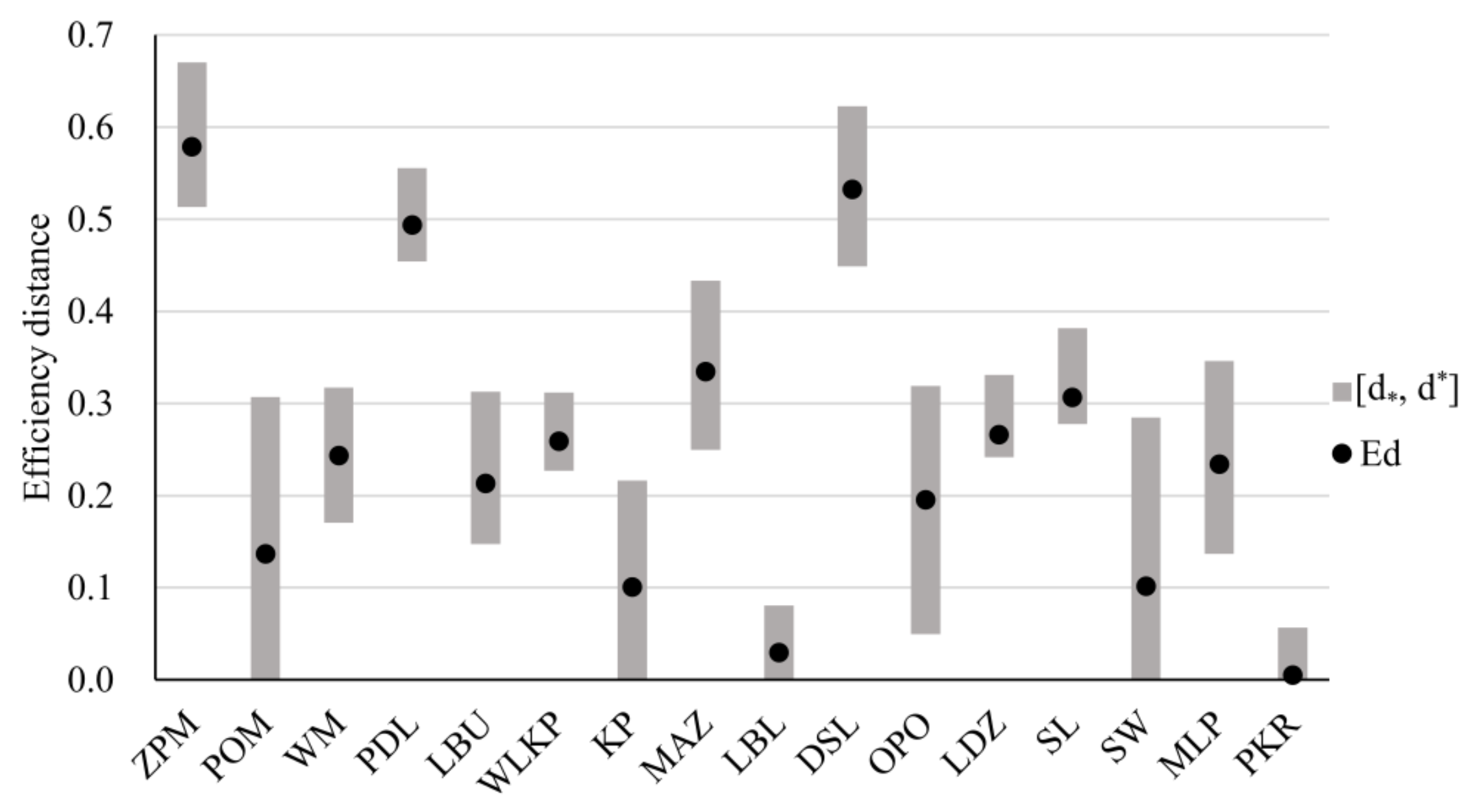
Figure 9 presents the extreme and expected distances to the best unit for all considered voivodeships. WLKP is the only efficient province given this category, so its distance to the best unit always equals zero. Hence, POM and LBU lose the status of efficient units. However, these two voivodeships and ZPM have relatively low distances to the best one: ZPM ($d^H\in [0.065,0.146]$), POM ($d^H\in [0.130,0.180]$), and LBU ($d^H\in [0.114,0.246]$). In general, the widths of distance intervals are notably more precise than when considering all relevant factors jointly. They are also more diverse, encompassing a greater range. In particular, seven provinces have maximal distances greater than $0.6$, with three even exceeding the threshold of $0.7$. At the comprehensive level, this was not observed for any voivodeship.

Among the inefficient provinces, ZPM can be considered the best, as it has the lowest distances to the best unit in both optimistic and pessimistic settings. Moreover, its best expected distance ($0.109$) is twice lower than at the comprehensive level, letting it overtake POM and LBU, which were judged efficient in the hierarchy’s root. The other twelve inefficient provinces are significantly worse. The least favorable among them is OPO, with the distance to the best unit in its optimistic scenario equal to $0.73$ and an expected distance of $0.754$. In the average case, OPO is directly preceded by MLP ($0.659$) and PKR ($0.652$). Note that at the comprehensive level, the worst maximal distances were attained by SL, DSL, and PDL. They all prove slightly better regarding inhabitants’ health improvement results.

Table 6. Distribution of distances to the best unit for Polish voivodeships when considering inhabitants’ health improvement level.

DAII	[0.0, 0.1]	(0.1, 0.2]	(0.2, 0.3]	(0.3, 0.4]	(0.4, 0.5]	(0.5, 0.6]	(0.6, 0.7]	(0.7, 0.8]	(0.8, 0.9]	(0.9, 1.0]
ZPM	0.332	0.668	0	0	0	0	0	0	0	0
POM	0	1	0	0	0	0	0	0	0	0
WM	0	0	0	0.055	0.727	0.218	0	0	0	0
PDL	0	0	0	0	0	0.658	0.342	0	0	0
LBU	0	0.713	0.287	0	0	0	0	0	0	0
WLKP	1	0	0	0	0	0	0	0	0	0
KP	0	0	0	0	0.341	0.659	0	0	0	0
MAZ	0	0	0	0.817	0.183	0	0	0	0	0
LBL	0	0	0	0	0.342	0.618	0.040	0	0	0
DSL	0	0	0	0.033	0.510	0.433	0.024	0	0	0
OPO	0	0	0	0	0	0	0	1	0	0
LDZ	0	0	0	0	0.150	0.710	0.140	0	0	0
SL	0	0	0.433	0.567	0	0	0	0	0	0
SW	0	0	0	0	0.256	0.744	0	0	0	0
MLP	0	0	0	0	0	0.088	0.715	0.197	0	0
PKR	0	0	0	0	0	0.125	0.708	0.167	0	0

presents the distribution of distances for all voivodeships when considering the inhabitants’ health improvement level. The only two provinces for which this distance is lower than $0.1$ are WLKP ($100\%$) and ZPM ($33.2\%$). Such a favorable result was not attained by ZPM at the comprehensive level for any feasible weight vector. Then, its distance could drop even above $0.4$. For the two units mentioned above, as well as POM and LBU, all samples confirm distances not higher than $0.2$. Furthermore, for all provinces, we can indicate a single bucket in which the unit’s distance falls for most samples. For example, it is $(0.2,0.3]$ for LBU, $(0.3,0.4]$ for MAZ, and $(0.7,0.8]$ for OPO. For these three provinces, the predominating distance buckets at the comprehensive level were better. However, for other voivodeships, including SW, MLP, and PKR, the most often repeated distance range worsened when limiting the analysis to the inhabitants’ health improvement level.

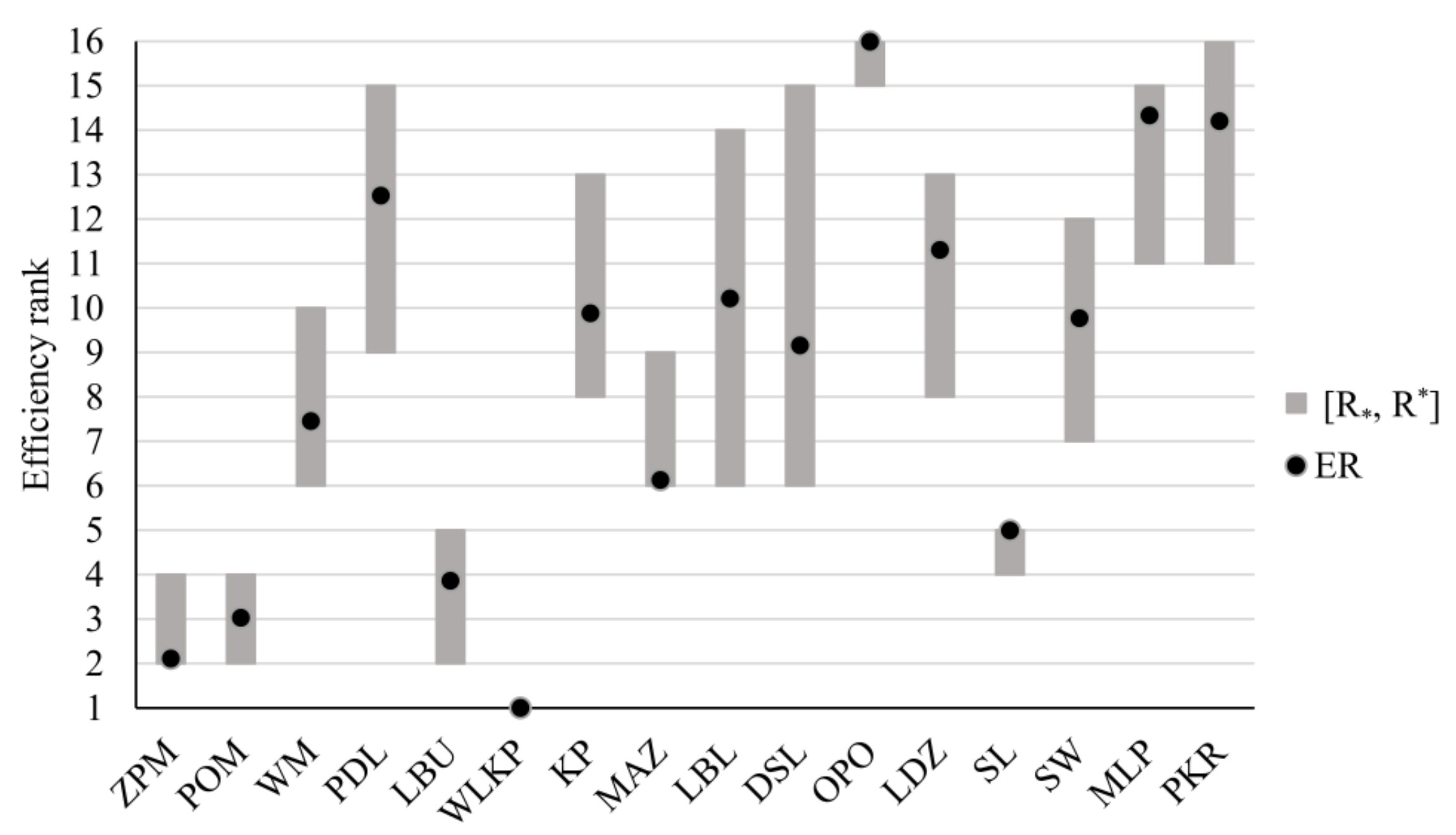
The extreme and expected efficiency ranks at the inhabitants’ health improvement level are provided in Figure 10. WLKP, as the only efficient province, is always ranked first. Both ZPM and POM are ranked between second and fourth, while for LBU, this range is slightly wider ($[2,5]$). Conversely, only two voivodeships—OPO and PKR—fall to the bottom ranking at any point, and three others (WM, DSL, and MLP) are ranked fifteenth in the least favorable scenario. Finally, for DSL and MAZ, the difference between their extreme ranks is the greatest. For example, DSL is ranked between sixth and fifteenth. According to the expected ranks, WLKP ($ER=1$), ZPM ($2.110$), POM ($3.034$), and LBU ($3.860$) are the best, and PKR ($14.205$), MLP ($14.339$), and OPO ($15.990$) are the worst.

When compared to the comprehensive level, the greatest improvement in the attained ranks can be observed for ZPM ($[2,4]$ rather than $[4,15]$) and SL ($[4,5]$ rather than $[7,16]$). On the contrary, the greatest deterioration of possible positions is noted for OPO ($[15,16]$ rather than $[8,16]$) and MLP ($[11,16]$ rather than $[4,15]$). For many provinces, including WM, POL, MAZ, LBL, LDZ, and SW, the ranking intervals got significantly narrower, confirming the lower diversity of results when limiting the scope of the analysis to health improvement.

The distribution of efficiency ranks given the inhabitants’ health improvement level is presented in

Table 7. Distribution of ranks for Polish voivodeships when considering inhabitants’ health improvement level.

ERAI	1	2	3	4	5	6	7	8	9	10	11	12	13	14	15	16
ZPM	0	0.916	0.058	0.026	0	0	0	0	0	0	0	0	0	0	0	0
POM	0	0.054	0.858	0.088	0	0	0	0	0	0	0	0	0	0	0	0
WM	0	0	0	0	0	0.029	0.705	0.110	0.093	0.063	0	0	0	0	0	0
PDL	0	0	0	0	0	0	0	0	0.003	0.179	0.096	0.075	0.403	0.142	0.102	0
LBU	0	0.030	0.084	0.882	0.004	0	0	0	0	0	0	0	0	0	0	0
WLKP	1	0	0	0	0	0	0	0	0	0	0	0	0	0	0	0
KP	0	0	0	0	0	0	0	0.212	0.272	0.182	0.087	0.247	0	0	0	0
MAZ	0	0	0	0	0	0.932	0.013	0.046	0.009	0	0	0	0	0	0	0
LBL	0	0	0	0	0	0	0.049	0.036	0.294	0.206	0.177	0.176	0.049	0.013	0	0
DSL	0	0	0	0	0	0.039	0.039	0.399	0.201	0.070	0.142	0.064	0.019	0.026	0.001	0
OPO	0	0	0	0	0	0	0	0	0	0	0	0	0	0	0.010	0.990
LDZ	0	0	0	0	0	0	0	0.120	0.059	0.085	0.159	0.281	0.296	0	0	0
SL	0	0	0	0.004	0.996	0	0	0	0	0	0	0	0	0	0	0
SW	0	0	0	0	0	0	0.194	0.077	0.069	0.215	0.311	0.134	0	0	0	0
MLP	0	0	0	0	0	0	0	0	0	0	0.023	0.011	0.043	0.450	0.473	0
PKR	0	0	0	0	0	0	0	0	0	0	0.005	0.012	0.190	0.369	0.414	0.010

. The most stable individual positions were observed for WLKP (1–$100\%$), SL (5–$99.6\%$), OPO (16–$99.0\%$), and ZPM (2–$91.6\%$). Such high acceptabilities were not observed at the comprehensive level for any position and unit. In fact, the greatest share of weights ($72.4\%$) supported the third position of LBU. Returning to the health improvement category, for some other voivodeships, the vast majority of weights indicate a pair of ranks (e.g., MLP and PKR are ranked 14th or 15th for $92.3\%$ or $78.3\%$ samples, respectively). Finally, the ranks of some units are more dependent on the chosen weight vector. For example, KP attained positions between 8th and 12th, with no $ERAI$ exceeding $28\%$. Similarly, SW is ranked within the range $[7,12]$ with $ERAI$s not less than $6.9\%$ and not greater than $31.1\%$. Still, these outcomes exhibit less diversity than at the comprehensive level.

The graph of the necessary relation at the inhabitants’ health improvement level is shown in Figure 11. The robust conclusions are richer than at the comprehensive level. For example, the number of pairs of different provinces that are related by the necessary preference increased from 47 to 85. Moreover, the number of levels in the respective Hasse diagram increased from 3 to 7.

In particular, WLKP is necessarily preferred to all other provinces, and four other voivodeships—POM, ZMP, LBU, and SL—proves to be necessarily better than the remaining eleven units. The worst unit is OPO, which is not necessarily preferred to any other province while being possibly preferred only to PKR. Further, MLP and PKR are necessarily worse than 10 and 9 other provinces, respectively. Finally, SL benefited the most from limiting the scope to the health improvement level, because in the hierarchy’s root, it was not robustly better than any other voivodeship.

The respective $PEOI$s are given in

Table 8. Pairwise efficiency outranking indices for pairs of Polish voivodeships when considering inhabitants’ health improvement level.

PEOI	ZPM	POM	WM	PDL	LBU	WLKP	KP	MAZ	LBL	DSL	OPO	LDZ	SL	SW	MLP	PKR
ZPM	1	0.948	1	1	0.973	0	1	1	1	1	1	1	1	1	1	1
POM	0.052	1	1	1	0.897	0	1	1	1	1	1	1	1	1	1	1
WM	0	0	1	1	0	0	0.995	0.070	0.904	0.921	1	0.851	0	0.786	1	1
PDL	0	0	0	1	0	0	0	0	0.240	0.014	1	0.320	0	0.209	0.844	0.767
LBU	0.027	0.103	1	1	1	0	1	1	1	1	1	1	0.987	1	1	1
WLKP	1	1	1	1	1	1	1	1	1	1	1	1	1	1	1	1
KP	0	0	0.005	1	0	0	1	0	0.565	0.395	1	0.640	0	0.524	1	0.996
MAZ	0	0	0.930	1	0	0	1	1	0.989	0.939	1	1	0	1	1	1
LBL	0	0	0.096	0.760	0	0	0.435	0.011	1	0.278	1	0.688	0	0.489	0.962	1
DSL	0	0	0.079	0.986	0	0	0.605	0.061	0.722	1	1	0.728	0	0.635	0.942	0.947
OPO	0	0	0	0	0	0	0	0	0	0	1	0	0	0	0	0.015
LDZ	0	0	0.149	0.680	0	0	0.360	0	0.312	0.272	1	1	0	0.011	1	1
SL	0	0	1	1	0.013	0	1	1	1	1	1	1	1	1	1	1
SW	0	0	0.214	0.791	0	0	0.476	0	0.511	0.365	1	0.989	0	1	1	1
MLP	0	0	0	0.156	0	0	0	0	0.038	0.058	1	0	0	0	1	0.478
PKR	0	0	0	0.233	0	0	0.004	0	0	0.053	0.985	0	0	0	0.522	1

. Similarly, as at the comprehensive level, for some pairs, one unit is significantly better than the other (see, e.g., ZPM and POM with $PEOI(ZPM,POM)=94.8\%$ or LBU and SL with $PEO{I}^H(LBU,SL)=98.7\%$). In turn, other pairs are characterized by more balanced stochastic acceptabilities, indicating an advantage of either voivodeship (see, e.g., PKR and MLP with $PEO{I}^H(PKR,MLP)=52.2\%$ or KP and SW with $PEO{I}^H(KP,SW)=52.4\%$). However, the absolute values of $POEI$s for some pairs differ vastly compared to the hierarchy’s root. For example, POM is necessarily better than ZPM at the comprehensive level, but when considering only health improvement, ZPM attains no worse efficiency for $94.8\%$ of feasible weights.

5.3. The Category of Financial Management

In this section, we discuss the results attained at the level of financial management. Instead of comparing them to the outcomes at the comprehensive level, we emphasize how managers can use them to improve the relative efficiency of provinces. Similar improvement strategies can be designed for other categories or hierarchy nodes.

Figure 12 presents the extreme and expected distances to the best province when limiting the scope to financial management. The most important result derived from their analysis is the division of provinces into efficient and inefficient. The minimal distance equals zero only for two units: POM and LBU. This means that they are the best performers among the sixteen voivodeships for at least one feasible weight vector. However, LBU has slightly better maximal and expected distances to the best province than POM. When looking at their inputs and outputs within the financial category, they perform equally well ($51.3$) on output $F_3$. It is the best value among all provinces. Moreover, the other two financial factors are greater for LBU, confirming that it transforms more beds (input $F_2$) into a more significant profit (output $F_1$). These two voivodeships should serve as ultimate peers for the remaining inefficient units in terms of financial management.

Among them, the overall good performers are WLKP ($E{d}^F=0.1689$) and MLP ($E{d}^F=0.2328$). They do not optimize one specific input or output, but perform decently on all indicators. In the optimistic, pessimistic, and expected scenarios, SL attains the least favorable results with the significantly greatest distances to the best province. In turn, KP has the broadest range of distances ($[0.140,0.416]$), confirming its performance’s sensitivity to the selection of particular priorities. This results from an imbalanced performance profile with a highly favorable value on output $F_1$ and a relatively poor value on output $F_3$. Finally, when complete order is desired, it can be imposed by the expected distances. In this case, LBU ($E{d}^F=0.010$) and POM ($E{d}^F=0.021$) are safely ranked at the top, and DSL ($E{d}^F=0.509$) and SL ($E{d}^F=0.735$) are ranked at the bottom.

The distance distribution at the financial management level is presented in

Table 9. Distribution of distances to the best unit for Polish voivodeships when considering financial management level.

DAII	[0.0, 0.1]	(0.1, 0.2]	(0.2, 0.3]	(0.3, 0.4]	(0.4, 0.5]	(0.5, 0.6]	(0.6, 0.7]	(0.7, 0.8]	(0.8, 0.9]	(0.9, 1.0]
ZPM	0	0	0	1	0	0	0	0	0	0
POM	1	0	0	0	0	0	0	0	0	0
WM	0	0	0.757	0.243	0	0	0	0	0	0
PDL	0	0	0.475	0.483	0.042	0	0	0	0	0
LBU	1	0	0	0	0	0	0	0	0	0
WLKP	0	0.993	0.007	0	0	0	0	0	0	0
KP	0	0.142	0.453	0.379	0.026	0	0	0	0	0
MAZ	0	0	0	0.857	0.143	0	0	0	0	0
LBL	0	0	0	0.139	0.775	0.086	0	0	0	0
DSL	0	0	0	0	0.312	0.688	0	0	0	0
OPO	0	0	0	0.240	0.708	0.052	0	0	0	0
LDZ	0	0	0.705	0.295	0	0	0	0	0	0
SL	0	0	0	0	0	0	0.220	0.743	0.037	0
SW	0	0	0.366	0.628	0.006	0	0	0	0	0
MLP	0	0.043	0.957	0	0	0	0	0	0	0
PKR	0	0	0	0	0.545	0.455	0	0	0	0

. For both efficient provinces (POM and LBU), the distance is always within the first bucket ($[0.0,0.1]$). Among the inefficient provinces, WLKP confirms its superiority over the remaining units, as for over $99\%$ samples, its distance from the efficient unit is not greater than $0.2$. The only two other provinces with positive $DAII$s for bucket $(0.1,0.2]$ are KP ($14.2\%$) and MLP ($4.3\%$). The greatest stability of distances among inefficient provinces is observed for ZPM with $DAI{I}^F(ZPM,(0.3,0.4])=1$. There are only two provinces, PDL and KP, for which most samples confirm no single distance bucket. Furthermore, KP is the only unit with positive $DAII$s for more than three buckets ($(0.1,0.5]$).

The results of the robustness analysis for efficiency ranks at the financial management level are presented in Figure 13 (extreme and expected positions) and

Table 10. Distribution of ranks for Polish voivodeships when considering financial management level.

ERAI	1	2	3	4	5	6	7	8	9	10	11	12	13	14	15	16
ZPM	0	0	0	0	0	0.011	0.046	0.182	0.062	0.624	0.068	0.007	0	0	0	0
POM	0.377	0.623	0	0	0	0	0	0	0	0	0	0	0	0	0	0
WM	0	0	0	0.048	0.318	0.207	0.089	0.143	0.195	0	0	0	0	0	0	0
PDL	0	0	0	0	0.001	0.206	0.200	0.205	0.133	0.164	0.091	0	0	0	0	0
LBU	0.623	0.377	0	0	0	0	0	0	0	0	0	0	0	0	0	0
WLKP	0	0	0.900	0.093	0.007	0	0	0	0	0	0	0	0	0	0	0
KP	0	0	0.100	0.088	0.248	0.169	0.066	0.077	0.074	0.061	0.117	0	0	0	0	0
MAZ	0	0	0	0	0	0	0	0.003	0.151	0.054	0.563	0.187	0.042	0	0	0
LBL	0	0	0	0	0	0	0	0	0	0.012	0.046	0.379	0.424	0.139	0	0
DSL	0	0	0	0	0	0	0	0	0	0	0	0	0	0.382	0.618	0
OPO	0	0	0	0	0	0	0	0	0.005	0.059	0.114	0.300	0.339	0.092	0.091	0
LDZ	0	0	0	0.100	0.126	0.365	0.332	0.077	0	0	0	0	0	0	0	0
SL	0	0	0	0	0	0	0	0	0	0	0	0	0	0	0	1
SW	0	0	0	0	0	0.013	0.267	0.313	0.380	0.026	0.001	0	0	0	0	0
MLP	0	0	0	0.671	0.300	0.029	0	0	0	0	0	0	0	0	0	0
PKR	0	0	0	0	0	0	0	0	0	0	0	0.127	0.195	0.387	0.291	0

(efficiency rank acceptability indices). They provide additional insights into the comparisons of efficient provinces. Specifically, even if LUB and POM can be ranked first for some weight vectors, the former is ranked first almost twice as often as the latter. This makes it the most favorable province regarding financial management, as additionally confirmed by the expected ranks ($E{R}^F(LUB)=1.377$ vs. $E{R}^F(POM)=1.623$). The remaining provinces are at most third in the best case. Again, WLKP proves to be the most advantageous among them, with $E{R}^F(WLKP)=3.107$. Further, KP has the broadest range of efficiency positions, being ranked between third and eleventh. $ERAI$s confirm that its ranks are rather equally distributed between these extreme positions, with the maximal value for the fifth rank ($ERA{I}^F(KP,5)=24.8\%$) and acceptabilities greater than $6\%$ for all ranks within the range $[3,11]$. Such great diversity is a consequence of its extreme performances. In fact, it is the best among all provinces on $F_1$ while being in the bottom three on $F_3$. Thus, KP is focused on the profit attained by healthcare institutions rather than on the number of treated patients. This aspect needs to be improved when aiming for higher ranks.

There are three other provinces with relatively wide possible efficiency rank intervals: ZPM ($[6,12]$), PDL ($[5,11]$), and OPO ($[9,15]$). Among them, only ZPM attains a single rank for most samples ($ERA{I}^F(ZPM,10)=62.4\%$). Finally, SL is ranked at the bottom regardless of the weight vector. This is related to its greatest value on input $F_2$, the lowest value on output $F_3$, and a relatively low value on output $F_1$. Thus, even if the financial input of SL is the greatest, its outputs are less favorable than for provinces with lesser financial resources. The complete ranking established with the expected efficiency ranks aligns with the one based on expected distances, with LBU, POM, WLKP, and MLP being ranked among the best provinces and SL, DSL, and PKR placed at the bottom.

Figure 14 presents the necessary ranking at the financial management level. POM and LBU are necessarily preferred to all other provinces, confirming their superiority given the financial category. The second level includes KP, WLKP, and MLP, and the lowest one contains PKR, DSL, and SL. They are possibly preferred to 4, 3, and 0 other units, respectively. Moreover, SL is necessarily worse than all other voivodeships.

The pairwise comparisons are useful for analysts particularly familiar with some provinces. For example, the authorities of OPO can compare it to other provinces searching for possible improvements. They can note that OPO is robustly worse than PDL or LBU and robustly better than SL. Notably, the necessary ranking (see Figure 14) is a good starting point to find the improvement paths for provinces. OPO has multiple paths to achieve efficiency. For example, it can take PDL as the first benchmark, follow WLKP, and finally refer to POM or LBU. An alternative improvement path runs through KP and POM.

The analysis of $PEOI$s (see

Table 11. Pairwise efficiency outranking indices for pairs of Polish voivodeships when considering financial management level.

PEOI	ZPM	POM	WM	PDL	LBU	WLKP	KP	MAZ	LBL	DSL	OPO	LDZ	SL	SW	MLP	PKR
ZPM	1	0	0	0.285	0	0	0.244	0.999	0.986	1	0.925	0.012	1	0.088	0	1
POM	1	1	1	1	0.403	1	1	1	1	1	1	1	1	1	1	1
WM	1	0	1	0.661	0	0	0.512	1	1	1	1	0.510	1	0.816	0.083	1
PDL	0.715	0	0.339	1	0	0	0.197	0.800	1	1	1	0.251	1	0.546	0.005	1
LBU	1	0.597	1	1	1	1	1	1	1	1	1	1	1	1	1	1
WLKP	1	0	1	1	0	1	0.920	1	1	1	1	1	1	1	0.996	1
KP	0.756	0	0.488	0.803	0	0.080	1	0.813	1	1	1	0.517	1	0.665	0.172	1
MAZ	0.001	0	0	0.200	0	0	0.187	1	0.932	1	0.809	0	1	0	0	1
LBL	0.014	0	0	0	0	0	0	0.068	1	1	0.480	0	1	0	0	0.752
DSL	0	0	0	0	0	0	0	0	0	1	0.102	0	1	0	0	0.287
OPO	0.075	0	0	0	0	0	0	0.191	0.520	0.898	1	0	1	0.006	0	0.754
LDZ	0.988	0	0.490	0.749	0	0	0.483	1	1	1	1	1	1	1	0.109	1
SL	0	0	0	0	0	0	0	0	0	0	0	0	1	0	0	0
SW	0.912	0	0.184	0.454	0	0	0.335	1	1	1	0.994	0	1	1	0	1
MLP	1	0	0.917	0.995	0	0.004	0.828	1	1	1	1	0.891	1	1	1	1
PKR	0	0	0	0	0	0	0	0	0.248	0.713	0.246	0	1	0	0	1

) is helpful for pairs related by mutual possible preference. For some, one province attains greater efficiency more often (e.g., $PEO{I}^F(SW,ZPM)=91.2\%$). For other pairs, indicating a better voivodeship is more challenging, as the shares of weights confirming the advantage of either unit are similar. An example of such a pair is LDZ and KP with $PEO{I}^F(LDZ,KP)=48.3\%$ and $PEO{I}^F(KP,LDZ)=51.7\%$.

5.4. The Category of Consumer Satisfaction

In this section, we present the results of provinces’ performance analysis at the level of consumer satisfaction with the healthcare system. To save space, we refer only to the exact and expected results without reporting the complete tables with stochastic acceptabilities.

Figure 15 presents the extreme and expected distances when considering the satisfaction of consumers. There are five efficient provinces with $d_{*}^S=0$: POM, KP, LBL, SW, and PKR. This is the greatest number for any node in the considered hierarchy. Among them, two provinces, LBL and PKR, have particularly narrow distance intervals, being close to the efficient units regardless of the weight vector ($d^{S,*}=0.081$ for LBL and $d^{S,*}=0.057$ for PKR). They are also the best regarding the expected distance (for PKR—$E{d}^S=0.005$ and for LBL—$E{d}^S=0.029$). In turn, the maximal (worst) possible distances for SW ($0.285$) and POM ($0.307$) are vastly greater, emphasizing their sensitivity to the selection of a particular weight vector. Among the inefficient units, the best minimal (optimistic) distance is achieved by OPO ($0.049$), and the best maximal (pessimistic) distance is attained by WLKP ($0.312$). The three provinces that are the worst considering both minimal and maximal distance are PDL ($d_{*}^S=0.454$, $d^{S,*}=0.556$), DSL ($d_{*}^S=0.449$, $d^{S,*}=0.623$), and ZPM ($d_{*}^S=0.513$, $d^{S,*}=0.670$). Their poor performance is also reflected in the bottom ranks according to the expected distances.

The extreme and expected efficiency ranks in consumer satisfaction are presented in Figure 16. Among the five efficient provinces, PKR has the narrowest rank interval; in the least favorable scenario, it is ranked third. On the contrary, even if POM is efficient, it can drop even to the tenth position, making its performance the least stable among all voivodeships. LBU is the best inefficient province when it comes to the best rank ($R_{*}^S=3$), and the best-ranked inefficient units in the pessimistic settings are WM, LBU, and OPO ($R^{S,*}=9$). The worst provinces considering both the minimal and maximal ranks are ZPM ($[15,16]$), PDL ($[14,15]$), and DSL ($[14,16]$). Notably, their rank intervals are very narrow. As far as the expected ranks are concerned, the best province is PKR ($1.426$), followed by LBL ($2.249$) and KP ($3.441$). On the other extreme, PDL ($14.192$), DSL ($14.988$), and ZPM ($15.820$) are the least favorable.

The necessary efficiency preference relation is presented as the Hasse diagram in Figure 17. The provinces form the multiple-level structure, with efficient ones (POM, PKR, LBL, KP, and SW) at the top. Among them, PKR and LBL are necessarily preferred to the most significant number of eleven other provinces, while POM proves robustly better than only six other provinces. Five other voivodeships (WM, LBU, OPO, WLKP, and MLP) are placed in the second level. All of them are necessarily preferred to four or five other provinces. Finally, DSL and ZPM are confirmed as the worst provinces, as they are not necessarily preferred to any other province. In fact, DSL is possibly preferred to only two other units (ZPM and PDL), while ZPM is at least as efficient for at least one weight vector only when compared to DSL.

5.5. Complete Efficiency Rankings of Voivodeships

The expected distances ($Ed$) and ranks ($ER$) allow for the construction of a complete ranking of voivodeships. In this section, we compare such orders with the ones obtained with the most commonly used ranking procedures for DEA, i.e., Cross-efficiency (CE) [30] and Super-efficiency (SE) [31]. We adapted them to a value-based additive efficiency model and ran it on each category of indicators.

The rankings generated by all four procedures for the level of inhabitants’ health improvement are provided in

Table 12. The voivodeships’ efficiency rankings imposed by four different measures at the level of health improvement: expected distance ($Ed$), expected rank ($ER$), cross-efficiency ($CE$), and super-efficiency ($SE$).

	ZPM	POM	WM	PDL	LBU	WLKP	KP	MAZ	LBL	DSL	OPO	LDZ	SL	SW	MLP	PKR
$Ed$	0.109	0.152	0.462	0.582	0.179	0.000	0.514	0.372	0.523	0.492	0.754	0.548	0.302	0.526	0.659	0.652
	2	3	7	13	4	1	9	6	10	8	16	12	5	11	15	14
$ER$	2.110	3.034	7.456	12.530	3.860	1.000	9.885	6.132	10.215	9.164	15.990	11.310	4.996	9.774	14.339	14.205
	2	3	7	13	4	1	10	6	11	8	16	12	5	9	15	14
$CE$	0.102	0.155	0.471	0.598	0.178	0.000	0.525	0.378	0.507	0.495	0.760	0.526	0.294	0.509	0.656	0.630
	2	3	7	13	4	1	11	6	9	8	16	12	5	10	15	14
$SE$	0.065	0.130	0.383	0.514	0.114	-0.140	0.458	0.324	0.414	0.374	0.726	0.470	0.233	0.469	0.565	0.560
	2	4	8	13	3	1	10	6	9	7	16	12	5	11	15	14

. To quantify the agreement level of such rankings for all hierarchy nodes, we used Kendall’s $\tau$ coefficient [28,32]. Its values are shown in

Table 13. Kendall’s $\tau$ coefficient for ranking procedures at each hierarchy level.

	Comprehensive Analysis				Inhabitants’ Health Improvement				Effective Financial Management				Consumer Satisfaction
	$\mathit{Ed}$	$\mathit{ER}$	$\mathit{CE}$	$\mathit{SE}$	$\mathit{Ed}$	$\mathit{ER}$	$\mathit{CE}$	$\mathit{SE}$	$\mathit{Ed}$	$\mathit{ER}$	$\mathit{CE}$	$\mathit{SE}$	$\mathit{Ed}$	$\mathit{ER}$	$\mathit{CE}$	$\mathit{SE}$
$Ed$	1.00	1.00	0.73	0.72	1.00	0.97	0.97	0.95	1.00	0.97	0.97	0.95	1.00	1.00	0.95	0.90
$ER$	1.00	1.00	0.73	0.72	0.97	1.00	0.97	0.92	0.97	1.00	0.97	0.92	1.00	1.00	0.95	0.90
$CE$	0.73	0.73	1.00	0.85	0.97	0.97	1.00	0.95	0.97	0.97	1.00	0.92	0.95	0.95	1.00	0.92
$SE$	0.72	0.72	0.85	1.00	0.95	0.92	0.95	1.00	0.95	0.92	0.92	1.00	0.90	0.90	0.92	1.00

. Note that $-1$ means the rankings are inverse, whereas 1 denotes a pair of the same rankings.

All four procedures provide highly correlated rankings. The two methods proposed in this paper ($Ed$ and $ER$) offer the most similar orders of provinces. The rankings constructed with these two procedures are the same for the comprehensive analysis of the healthcare systems and the customer satisfaction category. For the remaining two categories, Kendall’s $\tau$ coefficient equals $0.97$.

The similarity between the rankings based on $Ed$, $ER$, and CE is between $0.73$ for the comprehensive analysis and $0.97$ for health improvement and financial management perspectives. The average measure value is $0.904$. When comparing the orders imposed by SE and the two robustness-based methods, Kendall’s $\tau$ is between $0.72$ and $0.95$ ($0.92$) for $Ed$ ($ER$), with an average value of $0.879$ ($0.863$). Given that the maximal possible value of Kendall’s $\tau$ is 1, the observed similarity levels are very high.

5.6. Discussion

Three provinces, namely POM, WLKP, and LBU, prove to be the best in the comprehensive analysis of the healthcare system in Poland. However, the results for the three subcategories differ. This section discusses the conclusions that can be derived from the cross-category analysis, indicating various provinces’ strong and weak points. For illustrative purposes, we refer to three example voivodeships representing the top (WLKP), middle (PKR), and bottom (OPO) performers in the hierarchy’s root.

When it comes to WLKP, it proves to be the best at the inhabitants’ health improvement level; it is necessarily preferred by POM and LBU for the financial management level, and its ranks are between fifth and twelfth, given the consumer satisfaction perspective. This suggests that despite the decent quality of medical services, there is room for improvement in patient satisfaction and financial management. In particular, managers can conduct some training in soft skills for medical staff to improve consumer assessment of the healthcare system.

PKR is the best province regarding consumer satisfaction, as confirmed by its favorable expected distance and rank. However, when considering the comprehensive results and conclusions drawn for the remaining two categories, it performs poorly. Its expected rank is greater than 13 for inhabitants’ health improvement and financial management categories, while in the hierarchy’s root, its average rank is $12.024$. Hence, the healthcare system managers in this province should focus on improvements in medical decisions and financial management. In turn, other provinces can consider the healthcare system in PKR as the benchmark of proper communication with the consumers.

Such a cross-category analysis can serve as the basis for designing an improvement plan for provinces that proved to be relatively bad in the comprehensive analysis. In particular, the analysis of OPO’s poor performance points to the inhabitants’ health improvement category and financial management. It is the worst province for the former perspective for $99\%$ of weight vectors, and its expected rank is only $12.549$ for the latter category. Hence, managers should first focus on improving inhabitants’ health, due to the high importance of this category in the analysis. Then, they should design a plan for advancing financial management.

6. Conclusions

This paper introduce a novel framework for robustness analysis in the context of additive value-based efficiency analysis with a hierarchical structure. It admits a multiple-layer organization of relevant factors from the most general to the most detailed ones while tolerating both inputs and outputs in the same node. We accept the linear weight restrictions concerning the importance and trade-offs between various factors or subcategories with the common predecessor in the hierarchy. The results can be considered in each hierarchy node, letting the analyst view the comprehensive outcomes and draw conclusions for the subproblems where the relevant factors are limited to concise subsets of inputs and outputs reflecting a particular perspective. The proposed framework can be used in the standard efficiency analysis and the decision contexts requiring the consideration of composite indicators.

We derived the results by considering three perspectives: score-based distances to the efficient unit, ranks, and pairwise preference relations. For each of them, we proposed a pair of methods. The first group was based on mathematical programming, offering the exact, extreme outcomes that can be attained in the set of feasible input/output weights. The other group was based on Monte Carlo simulations, providing the distribution of efficiency outcomes through stochastic acceptabilities that estimate the share of the weight subspaces confirming a given result. These approaches are complementary because the exact outcomes often need more conclusiveness, whereas the stochastic indices—even if approximated with high accuracy—may fail to capture some extreme results.

We illustrated the framework’s applicability by assessing the quality of the healthcare system of sixteen Polish voivodeships. The analysis included nine indicators of different natures and concerned four levels. The comprehensive results were based on all relevant characteristics considered jointly, while the three subproblems captured the perspectives of inhabitants’ health improvement, financial management, and consumer satisfaction. We reported three provinces—Pomorskie (POM), Wielkopolskie (WLKP), and Lubuskie (LBU)—as the most efficient ones. We presented their strong and weak points by referring to the results in all hierarchy nodes. Moreover, we discussed the practical usefulness of the robustness analysis in terms of managerial implications.