Article

Challenges and Recommendations for Improved Identification of Low ILUC-Risk Agricultural Biomass

1
Cerulogy, London WC2H 9JQ, UK
2
Centre for Environmental Policy, Imperial College London, Exhibition Road, London SW7 2AZ, UK
*
Author to whom correspondence should be addressed.
Appl. Sci. 2023, 13(10), 6349; https://doi.org/10.3390/app13106349
Submission received: 24 February 2023 / Revised: 11 May 2023 / Accepted: 18 May 2023 / Published: 22 May 2023

Abstract

:
The “low indirect land use change risk” (“low ILUC-risk”) concept was developed to assess whether crop-based biofuels would compete with other land uses and cause the expansion of agricultural land. At the core of low ILUC-risk is an “additionality principle”, which requires that biofuel feedstock receive special treatment only if it is produced over and above the business-as-usual baseline. This paper examines and tests the European Commission’s methodology for calculating the baseline for yield improvement projects, by applying it to publicly available Eurostat data at national and NUTS2 scales. We assess from a statistical perspective how variation in regional yield trends would lead to differences in the long-term outcomes of low ILUC-risk certification; we conclude that, as currently designed, the methodology would over-state the amount of additional production in some cases and could hence incentivise the diversion of crops from other uses into the biofuel sector. We introduce the terms “tailwind additionality”, “headwind additionality”, and “additionality ratchet” to characterise the phenomena which contribute to this outcome. Our results lead us to recommendations which may enhance both the attractiveness and the robustness of the low ILUC-risk system.

1. Introduction

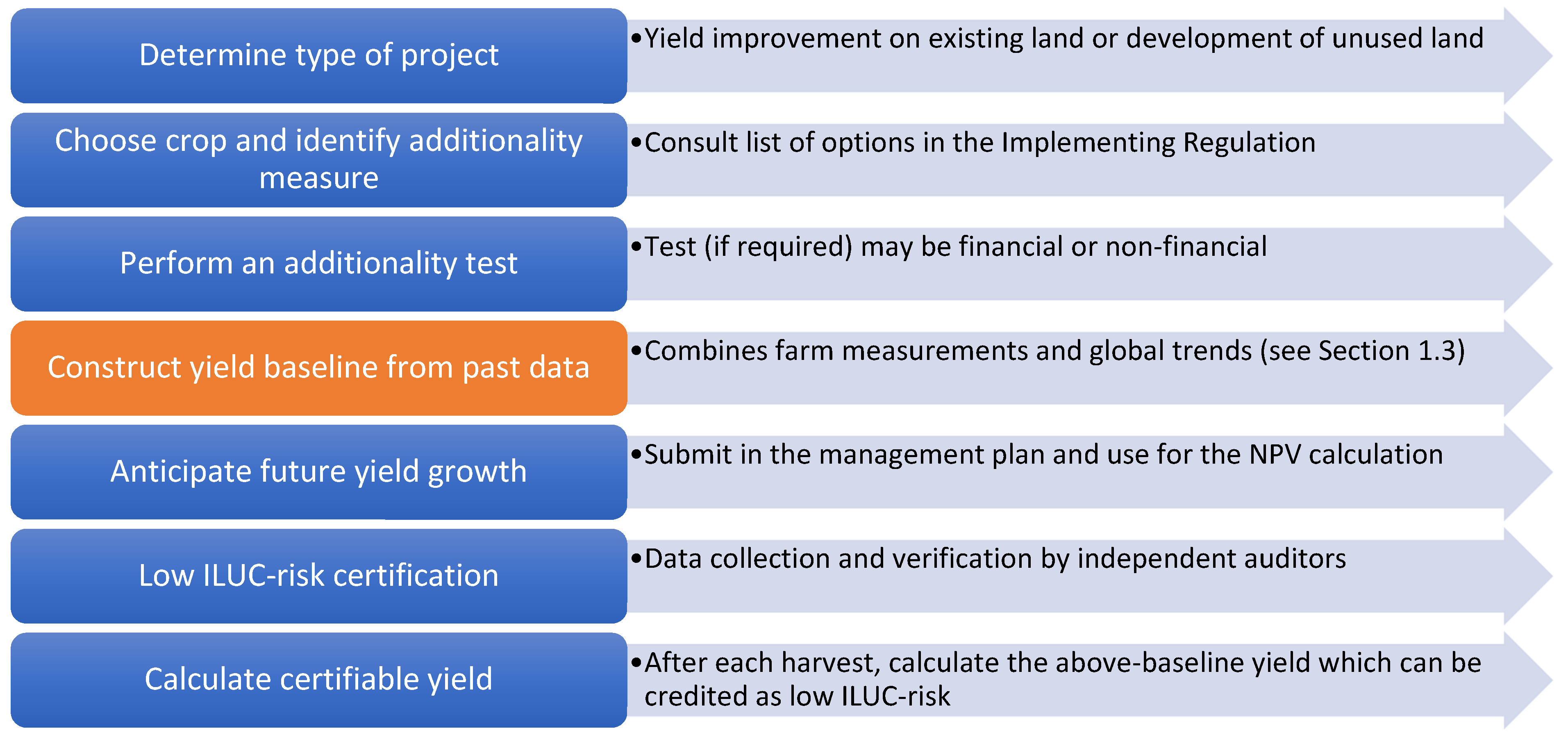
1.1. The Low ILUC-Risk Concept

A major concern surrounding crop-based biofuels is that they compete with other uses for land and feedstock. In the short term, this may reduce the supply of food and hence raise prices; in the longer term, it could drive agricultural land expansion, with associated emissions from changing land use.
This second phenomenon, where high commodity prices result in agricultural expansion into formerly unfarmed areas, is called “indirect land use change” (ILUC) [1,2,3]. In some cases, this leads to conversion of lands with high carbon stocks, for instance forests and wetlands; in other cases, it affects land such as pasture or scrubland which have lower carbon stocks but which, in aggregate, may still result in high levels of greenhouse gas emissions.
The European Commission has determined that estimates of ILUC emissions from given crops are not robust enough to be used in regulatory lifecycle analysis [4,5]. In the context of calculating the lifecycle emissions of biofuels, the recast Renewable Energy Directive (“RED II”) states that [6]:
the level of greenhouse gas emissions caused by indirect land-use change cannot be unequivocally determined with the level of precision required to be included in the greenhouse gas emission calculation methodology’.
To get around this issue, the Commission has developed two concepts to identify which feedstocks are likely to be associated with ILUC emissions [7,8]. First, feedstocks which are associated with large-scale expansion into high-carbon land are designated “high ILUC-risk”; biofuels made from these feedstocks are to be phased out of EU renewable energy targets. Second, “low ILUC-risk” feedstocks are those produced through methods which cause no additional demand for land. Specifically [9] (emphasis added):
Biofuels, bioliquids or biomass fuels should be considered low ILUC-risk only if the feedstock used for their production is cultivated as a result of the application of duly verifiable measures to increase productivity beyond the increases which would be already achieved in a business-as-usual scenario’.

1.1.1. Additionality

The requirement that low ILUC-risk feedstock should go beyond the business-as-usual production is known as “additionality” [10,11,12]. This section outlines the set of rules developed by the European Commission for assessing additionality in crop production; we refer to this as the “Commission methodology” or the “RED II methodology” interchangeably, and we note that it is already being operationalised by sustainability certification bodies to award low ILUC-risk certificates at the farm level. The objective of this paper is to study the practical implications of the Commission’s methodology; this will be elaborated in Section 1.2 below.
The RED II and subsidiary texts specify three stages of additionality screening for low ILUC-risk certification. In the first stage, the feedstock producer must implement an “additionality measure” on their land (second box in Figure 1); this means [9]:
any improvement of agricultural practices leading, in a sustainable manner, to an increase in yields… on land that is already used for cultivation…; and any action that enables the cultivation of… crops on unused land, including abandoned land, for the production of biofuels, bioliquids and biomass fuels’.
From this, we may identify three broad types of low ILUC-risk projects, according to what kind of additionality measure was employed in order to achieve higher overall productivity. These types are:
(i)
projects which increase yields from existing crop cycles, by improving the efficiency and targeting of the agricultural management practices;
(ii)
projects which increase land productivity by adopting new types of cropping systems and rotations (e.g., intercropping and sequential cropping); and
(iii)
projects which bring formerly unused or abandoned land into production, while minimising any associated environmental impacts.
The requirement that an additionality measure is implemented ensures that some extra effort has been made on the part of the biomass producer to boost yields; this limits the potential for “free riding” on yields that would have risen anyway [7]. Examples of additionality measures include adoption of new seed varieties, introduction of sequential cropping, and investment in new machinery. A review of relevant practices and crops which may be financially and agronomically suitable for low ILUC-risk production in Europe can be found in [13].
The second stage of additionality screening evaluates the evidence that whatever additionality measure has been undertaken would not have been undertaken as a matter of course, i.e., that some barrier to implementation prevents the farmer from adopting the improved practices (third box in in Figure 1). The rationale is that, even if steps have been taken to improve agricultural practices, these may be part of business-as-usual trends aimed at meeting increasing demand from food and other markets; any extra production arising from such measures should not be diverted to the biofuel sector if ILUC is to be avoided. In many situations, a project can pass this stage of screening by showing that the net present value (NPV) of the candidate low ILUC-risk project is negative in the absence of incentives from the bioenergy sector. A negative NPV means that the proposed project would not be financially viable on its own, and hence that it would not go ahead under business-as-usual conditions; it only becomes attractive because of extra demand from the renewable energy sector.
For the third stage of additionality screening (the highlighted fourth box in Figure 1), the low ILUC-risk rules specify that certification applies only to the fraction of the yield which surpasses business-as-usual performance; this in turn is determined by the “dynamic yield baseline”, discussed in more detail in Section 1.3. The amount of yield that qualifies as additional depends both upon the success of the additionality measure and upon other external factors that affect the yield with respect to the baseline (e.g., good weather, other changes in management practices). If the additionality measure is successful and growing conditions are unusually favourable, then the amount of certifiable material could be significant. Conversely, if the yield achieved in a given year is at or below the calculated baseline then no material from the growing area in question can be certified as low ILUC-risk (there is no penalty if yields fall below the baseline). For biofuel feedstock production on unused or abandoned land (point (iii) in the list above), the baseline is zero, meaning that any biomass produced from such projects is considered additional and can be certified as low ILUC-risk, provided of course that the project meets all other certification requirements.

1.1.2. Results-Based Crediting

The focus of this study is the final stage of the low ILUC-risk additionality screening discussed in Section 1.1.1; i.e., the highlighted box in Figure 1, which is where applicants for low ILUC-risk certification (more specifically, those undertaking “yield improvement”-type projects on existing agricultural land; see points (i) and (ii) in the list above) must construct a yield baseline from their historical yield data.
The method of comparing a farm’s actual yields with a pre-determined baseline makes the low ILUC-risk system an example of “results-based” crediting, where incentives are coupled to demonstrated outcomes; here, the outcome is the amount of above-baseline feedstock production. Results-based crediting can be contrasted with “practice-based” crediting, where incentives are given simply for adopting practices which are likely to be beneficial. An example would be the greening payments of the EU’s Common Agricultural Policy (CAP).
A results-based low ILUC-risk scheme offers some certainty to buyers and society at large that a given batch of biofuel feedstock has avoided stimulating agricultural expansion, and hence comes with environmental benefits compared with a non-certified batch. However, the results-based framing is less attractive to producers, who in the face of uncontrollable weather conditions can predict neither the success of their additionality measure nor their future production. There is also a danger that a purely results-based scheme, when combined with variability over time and across geographies, may end up certifying business-as-usual production if temporary fluctuations are able to masquerade as yield improvements according to the comparison baseline (this is known as a “free-riding problem”).
In light of these issues, hybrid schemes which combine elements of both results- and practice-based approaches are sometimes appropriate [7]. Indeed, the low ILUC-risk methodology goes some way to incorporating practice-based conditions, as farmers must demonstrate adoption of an additionality measure, and their anticipated yield increase must be plausibly connected to this measure. This mitigates free riding to some extent (to be further explored in this study), but it still leaves producers to shoulder the uncertainty of weather variability.

1.2. This Paper

In this paper, we examine the RED II’s methodology for constructing yield baselines for low ILUC-risk “yield improvement” projects, by applying it to real-world historical data. This allows us to ask, “What would have happened if a typical farm in location X had gained low ILUC-risk certification in year Y and is this consistent with the intentions of the low ILUC-risk system?”. We thereby build a picture of the methodology’s strengths and weaknesses—including how it might be abused by bad-faith actors—in practical scenarios where agricultural productivity is subject to both long-term trends and annual variation.
More specifically, we use the publicly available Eurostat dataset on crop productivity (more on this in Section 2.1), which allows us to make judgements based on historical yield trends and draw conclusions at the sub-national NUTS2 level. As we shall see, low ILUC-risk certification applies at the farm (or even the field) level, which is more granular than the national and district scales considered here, and has greater levels of geographical, annual, and secular variation. Nevertheless, there is much to be learned about the RED II methodology from analysing larger-scale historical trends, and we can think of the yield dataset as representing a “typical” farm in each country or district. The use of NUTS2 data gives us the highest possible geographical resolution without undue sacrifice of accuracy and coverage.

1.3. Dynamic Yield Baselines

Feedstock production must surpass the baseline estimate of “business-as-usual” yield in order to be certified as low ILUC-risk. Constructing this baseline is, as with all counterfactuals, non-trivial, especially since localised data may not be available and weather variability can make it hard to discern long-term trends. Nevertheless, the low ILUC-risk texts stipulate the methodology for constructing a “dynamic yield baseline” for both annual and perennial crops and make provisions for multi-year rotation cycles and the adaptation of new crops into existing cycles. Note that the word “dynamic” here means that the value of the yield baseline changes in time, based on historical production trends. A “static” baseline would be fixed at a constant yield value. Examples of static baselines for low ILUC-risk frameworks are provided by ICAO’s CORSIA and the RSB (see Section 3.3).
In this paper, we consider the simplest agricultural model (from the perspective of the RED II methodology): annual main crops in a one-year rotation on the same plot, with a stable off-season land use. For this case, constructing the yield baseline for a given crop on a given plot of land happens in two steps: first, a farm-specific initialisation point, and then a universal extrapolation [14].
  • Initialisation point. The crop yield on the plot of land under consideration is averaged over (at least) the previous three years.
  • Extrapolation. From this initialisation point, future yields are linearly extrapolated using the global average yield growth for that crop, based on the last 10 years (at least) of data.
For the initialisation step, the Implementing Regulation [14] provides guidance in case accurate data at the farm level are missing, or if one of the years is considered non-representative. These provisions and their flexibilities are worthy of further discussion; however, in this paper we focus on the slope of the baseline (from the second step), the calculation of which has far-reaching consequences for how much crop production will be certifiable as low ILUC-risk.

Global Yield Trends

Historical records show that, over decadal timescales, many crops experience yield growth that can be well described by a linear trendline. This is observed at global, national, and regional scales, and emerges from the combination of climatic and ecological evolution as well as various local drivers, including expanding access to new crop varieties, harvesting machinery, irrigation technology, pest control, and soil nutrient management techniques.
The Implementing Regulation methodology recognises that, in order to ensure that agricultural production certified as low ILUC-risk is genuinely additional, it must go beyond these long-term background trends. Specifically, applicants for low ILUC-risk status must compare their yields against a dynamic baseline based on the “global average yield slope”, that is, the gradient of the straight line fit to global annual yields recorded in the FAOstat database (global annual yield, measured in units of t/ha/yr, means the total crop production (in tonnes, t) divided by the total harvest area (in hectares, ha), for a given year). Yield slopes for selected major crops such as wheat are calculated and tabulated in the Implementing Regulation (namely, for barley, maize, oil palm fruit, rapeseed, soybeans, sugar beet, sugar cane, sunflower seed, and wheat). For crops not included in this table, the yield slope must be calculated afresh using the most recent FAOstat data spanning at least 10 consecutive years. See Annex C in the Supplementary Material for an updated list of crops and yield slopes.
The low ILUC-risk dynamic yield baseline is constructed to follow such linearised global trends for each crop. The Commission’s rationale for this may have come from a sense that, as ILUC is a global market-mediated phenomenon, it is global rather than local trends in productivity that are relevant to assessments of additionality. A more prosaic motivation would be that many countries do not collect accurate yield statistics, either for major crop categories, such as wheat, or for novel bioenergy crops. Taking the global average is then the most universally consistent approach which maximises the amount of data going into the baseline.

2. Materials and Methods

2.1. Eurostat Crop Production

A primary goal of this study is to explore how the public Eurostat data can be used to inform agricultural and energy policy. The specific dataset in question is apro_cpshr (https://ec.europa.eu/eurostat/web/products-datasets/-/apro_cpshr (accessed on 11 May 2023)), which contains the annual production and harvested area for a number of crops at the national, “NUTS1”, and “NUTS2” levels. Here, “NUTS” stands for “Nomenclature of Territorial Units for Statistics”, a system for dividing and sub-dividing regions of the EU. The finest geographical resolution with adequate data is NUTS2, representing districts with populations between 800,000 and 3 million (https://ec.europa.eu/eurostat/web/nuts/principles-and-characteristics (accessed on 11 May 2023)).
The dataset features 68 distinct crop categories. Some of these are very broad (e.g., “leguminous plants”, “other cereals”), while some crop categories are derived from other categories (e.g., “barley” may be a composite of “winter barley” and “summer barley”). For this study, we identified 14 crop datasets of interest; see Figure 2. Further discussion is featured in Annex B of the Supplementary Material.
The dataset covers the entire EU, plus the UK and other peripheral countries (e.g., Albania, Switzerland, Ukraine, etc.). In total, 37 countries are represented. The number of NUTS2 districts is a little trickier to quantify, as these have shifted over time as a result of merging, splitting, deforming, and renaming. As of the last re-districting in 2021, there are 242 NUTS2 districts within the EU27.
The time period we cover is 2000–21 at the national level, and 2000–20 at the district level (we truncate the datasets a year early for reliability).

2.2. Cleaning and Filtering

In the data cleaning stage, the Eurostat database is fed into the processing pipeline represented in Figure 3 and described in more detail in Annex A of the Supplementary Material. For this study we restrict focus to large countries in the EU27 + UK and select crops which are (or are representative of) potential biofuel feedstocks. The final output of the cleaning pipeline is a dataset of annual yield values, indexed by region and crop.
This cleaned dataset is still patchy. Some data are missing because countries joined the EU more recently than 2000; some are missing because reporting requirements have changed over time; some are missing because certain crop types are not grown in all districts, and these appear as gaps in the record; still others may be missing because of non-reporting. It is beyond the scope of this study to determine the reasons and impacts of data gaps; these remarks are included merely as a warning that inferences may in some cases be based on incomplete records. Nevertheless, our overall findings and conclusions will still stand in spite of data gaps.

2.3. Analyses Presented

Ideally, the low ILUC-risk framework should reliably reward genuinely additional production while delivering a low rate of false positives. This study applies the methodology to data series from the Eurostat dataset to see whether this would have been the case historically, i.e., we consider how much material could have been credited as low ILUC-risk over a given historical period if low ILUC-risk certification had been around at that time. Alignment between our expectations and the analysis results would point to a well-functioning methodology, while any large discrepancy points to some problem.
As we shall see, the critical quantity for each crop in each district is its “yield slope”, that is, the long-term rate of yield growth (or decline) which is found through a linear least-squares fit (after eliminating outliers); this is visualised below in Figure 4. All the crops featured in Figure 2 are analysed, though in our presentation of results it is often convenient to focus on a single crop. Unless otherwise stated, all averages and fits are calculated over the whole time period for which data are available.

3. Results

This section presents our statistical analyses of the Eurostat data at both the national and the district level. We examine:
(i)
How past yield trends in different countries compare with the global average.
(ii)
The potential for such trends to return spurious above-baseline production under the low ILUC-risk system, purely on the basis of geography.
(iii)
The impact of year-on-year yield variability in the production of creditable low ILUC-risk feedstock.
(iv)
How the choice of baseline slope affects the production of creditable low ILUC-risk feedstock.

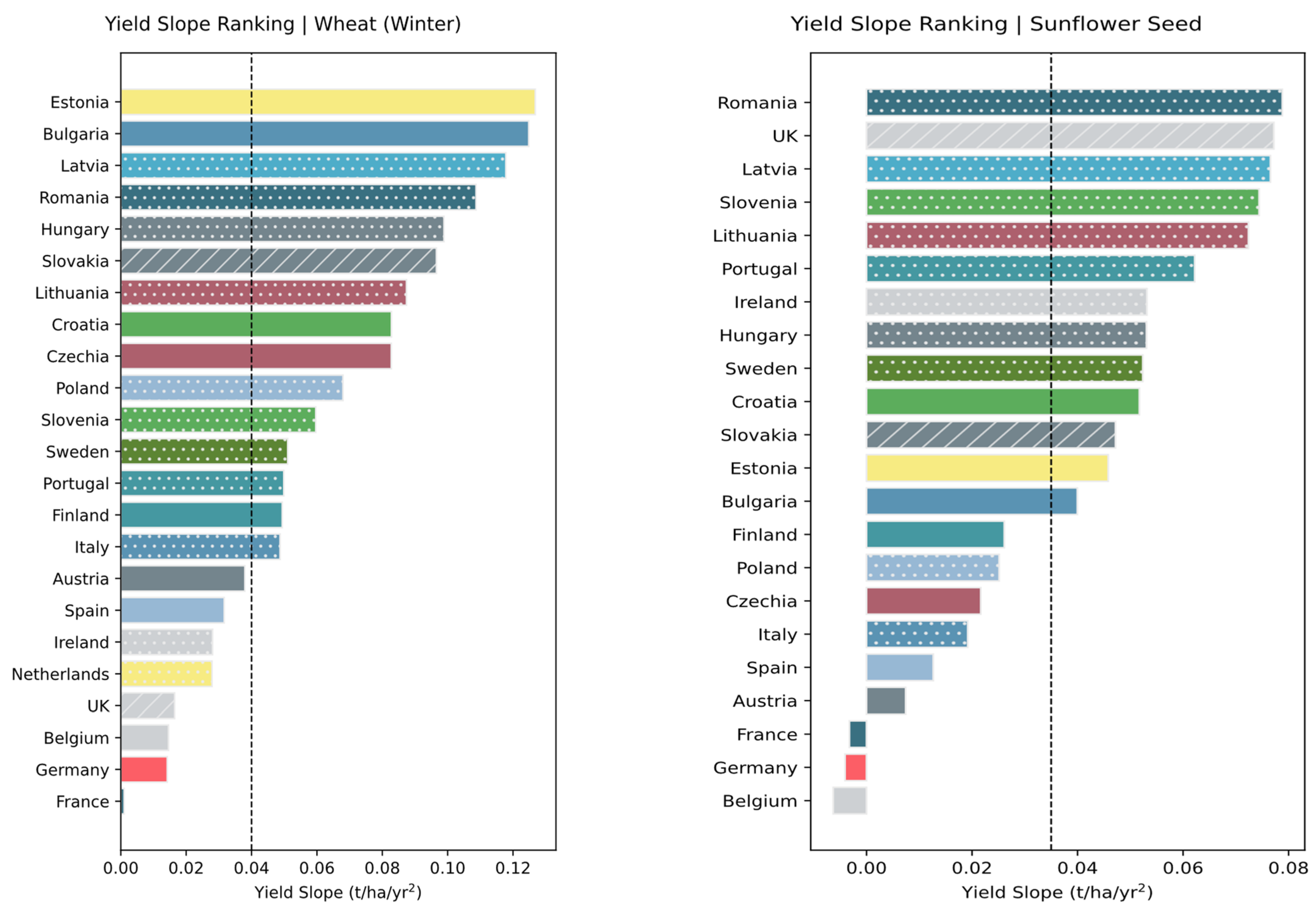
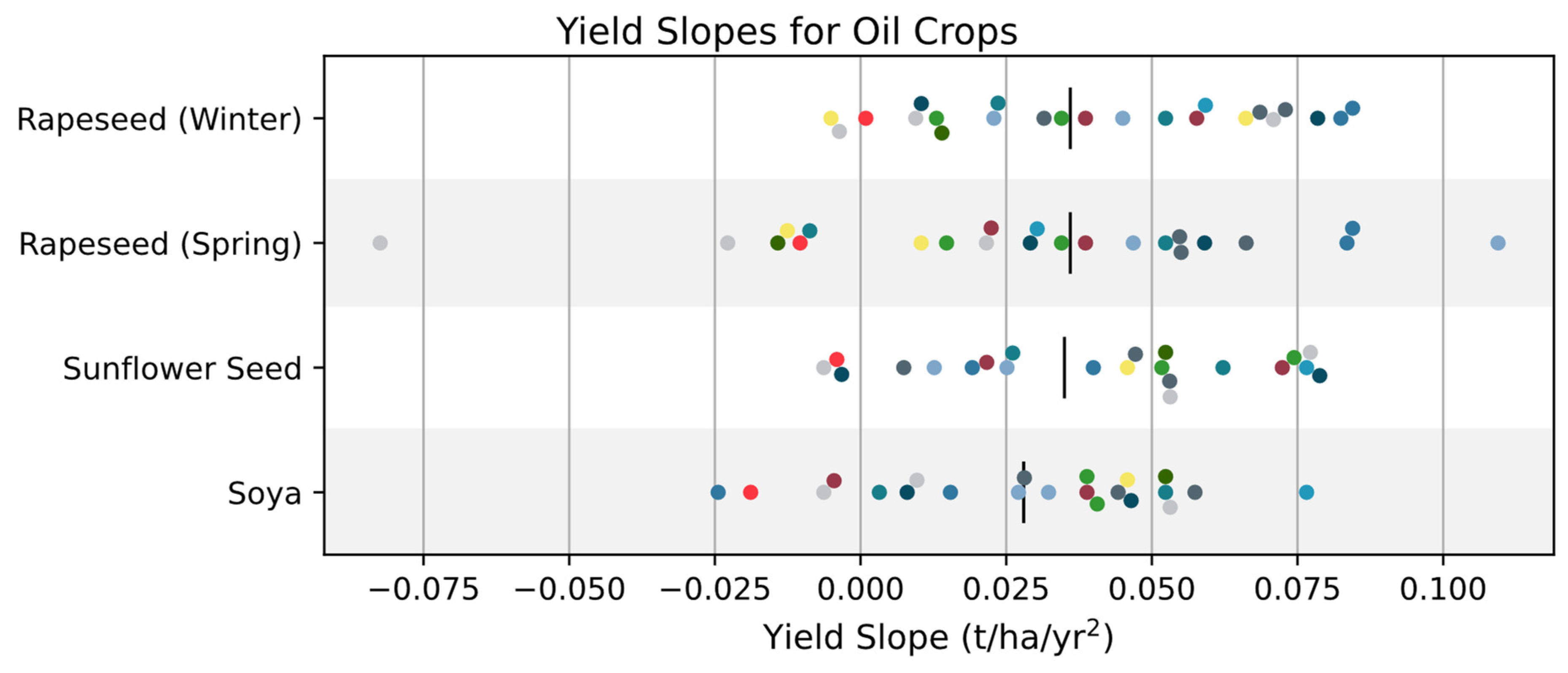
3.1. National Yield Trends

3.1.1. Yield Growth

The amount of low ILUC-risk feedstock that can be certified from a given farm depends on the difference between the farm’s actual yields and the dynamic yield baseline, which is based on the global average. In this spirit, this section analyses national-level trends in yield growth compared with the global average. The examples in Figure 4 show the fluctuating annual yields in the period 2000–21 (points), overlaid with the best fit line. The global average, calculated from FAOstat data according to the RED II methodology set out in the Implementing Regulation [14], is indicated as a black dashed line for comparison.
It is evident that some countries’ slopes are greater than average (e.g., Bulgaria, which roughly doubles its yield over 20 years), and some are less (e.g., Germany, where yields are more static). There are many contributing factors to a country’s yield growth, and it comes as no surprise that some countries out-perform others. Some of the factors are within the control of farmers themselves (possibly supported by national governments), such as improving mechanisation, adoption of appropriate crop varieties, targeting of chemical inputs, soil improvement measures, irrigation management, and protection against pests and diseases. Other factors are environmental and can’t be fully controlled at farm level; these include long-term changes in rainfall and temperature patterns and disease prevalence.
Figure 4. National annual yield for winter wheat for selected countries, with best fit slopes in the legend and the FAO global average slope for comparison.
Applsci 13 06349 g004
In Figure 5, the analysis in Figure 4 is extended to all countries offering sufficient data, with yield slopes presented over the period 2000–21 (note that throughout this paper, each country will be assigned to a consistent colour; for example, the dark blue for Bulgaria in Figure 4 is the same dark blue in Figure 5). The global average is indicated for comparison. Naturally, some countries’ yield slopes are greater than the global average, and some are smaller.

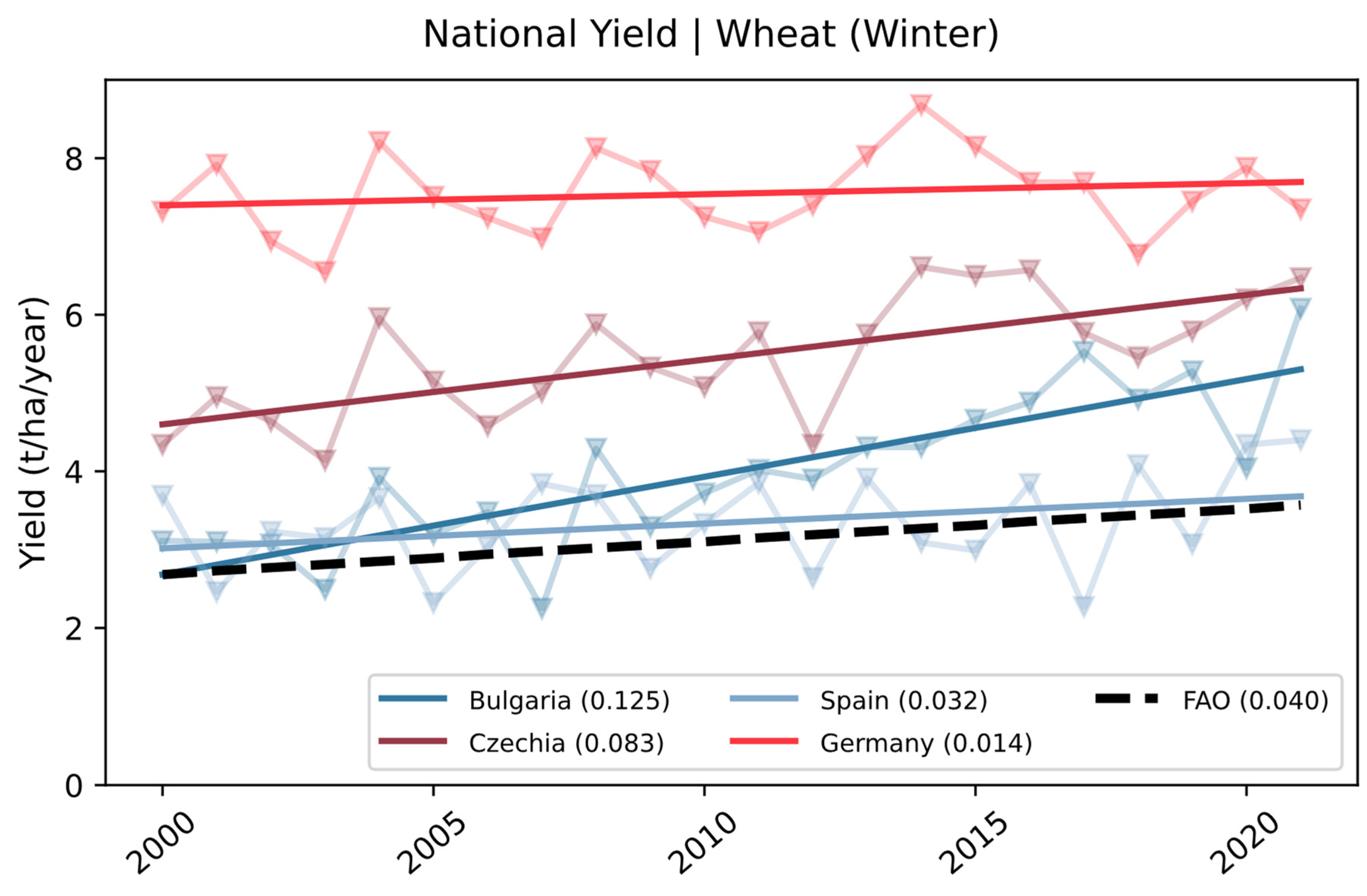
3.1.2. “Tailwind Additionality” and “Headwind Additionality”

Historical yield trends which are seen to depart from the global average have, of course, done so in the absence of any value signal from the low ILUC-risk system, which is a recent development. The fact that countries with high background yield growth have been able to surpass the global average means that typical projects in these countries would have been able to beat the dynamic yield baseline with relatively little exertion. Conversely, farmers in areas with low background yield growth may struggle to achieve certifiable additional material, regardless of any genuine efforts to do so. We invoke the terms “tailwind additionality” and “headwind additionality” to convey the respective advantage and disadvantage these farmers experience from long-term background trends.
Figure 6 and Figure 7 condense the information about national-level yield slopes, for cereal and oil crops, respectively. Countries are represented as points, using their assigned colours to help distinguish them, and there is one row for each crop. Yield slope is plotted along the horizontal axis, with points further to the right having higher slope (e.g., in the first row for winter wheat, the points for Estonia and Bulgaria are at the far right, in keeping with their ranking in Figure 5). The FAOstat global average is represented for each crop as a vertical black line. Countries to the right of this line experience a tailwind, and those to the left experience a headwind.

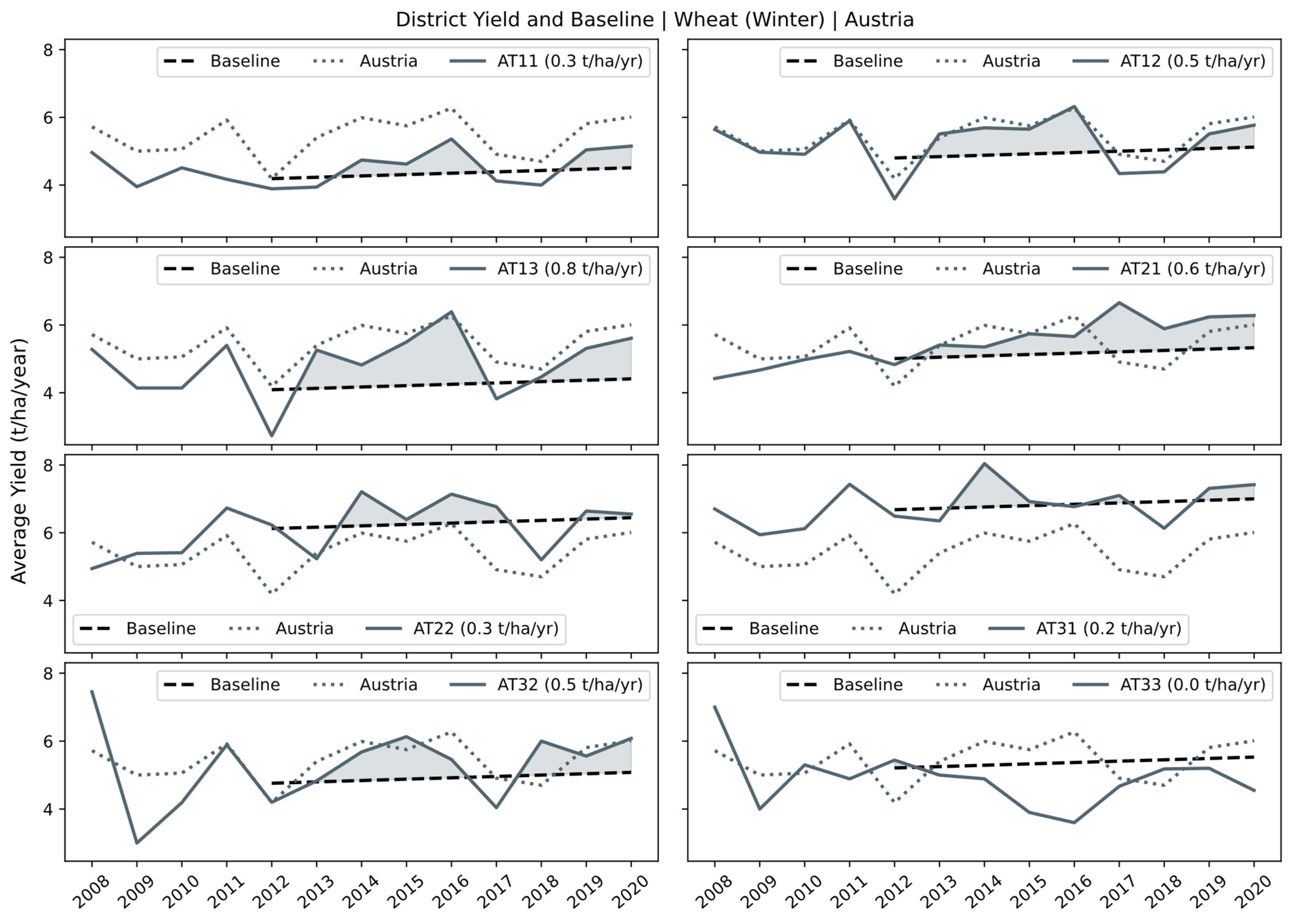
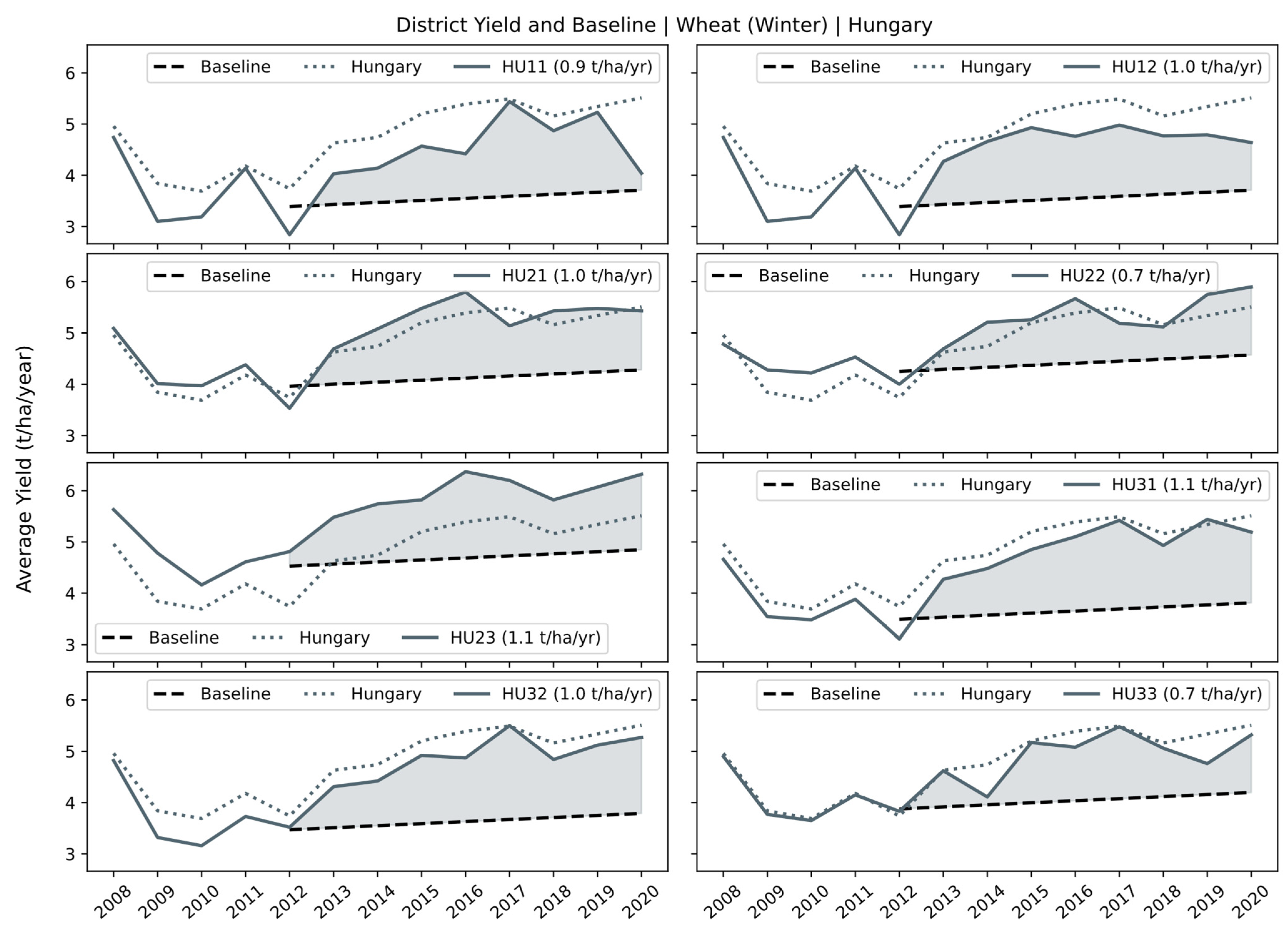
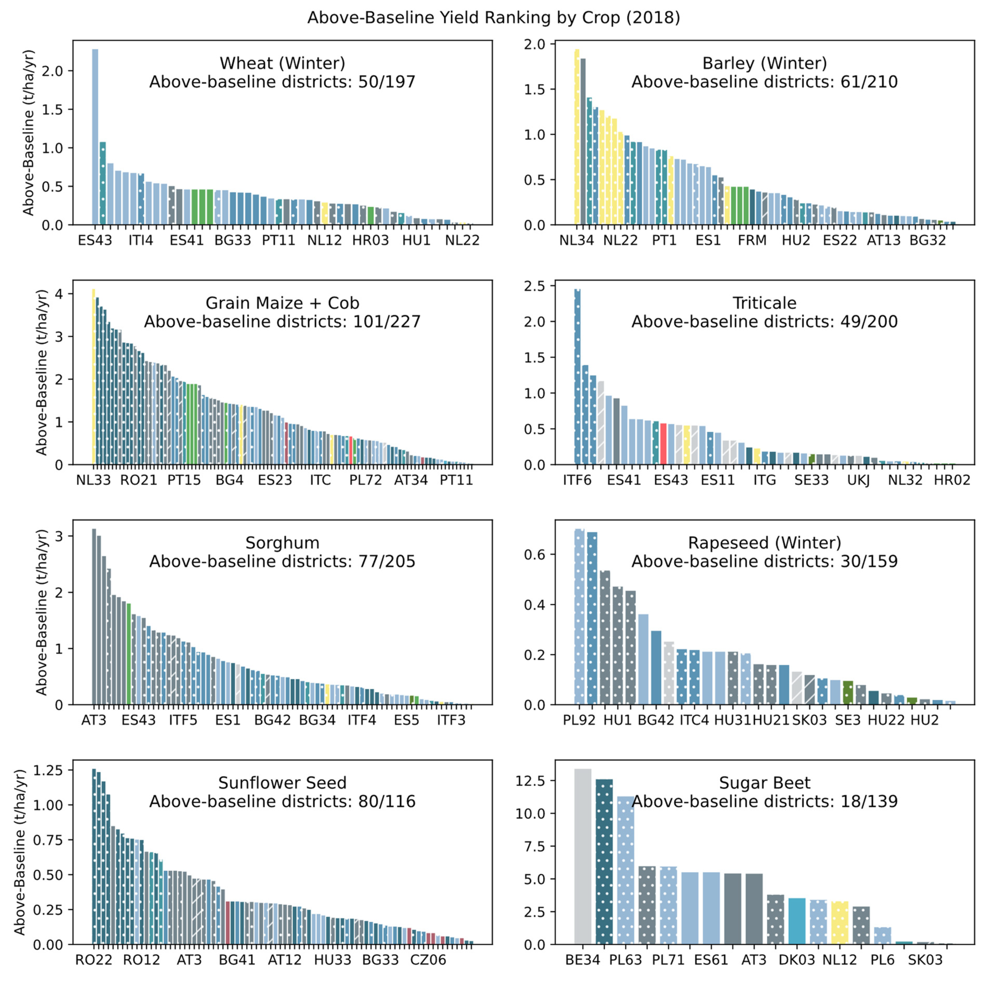
3.2. District-Level Above-Baseline Production

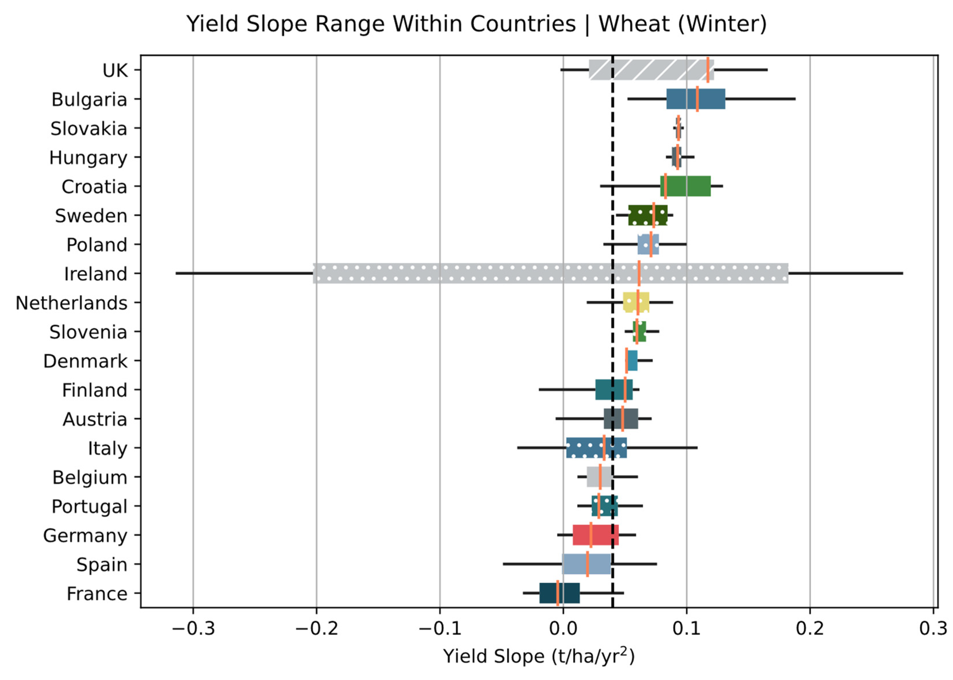
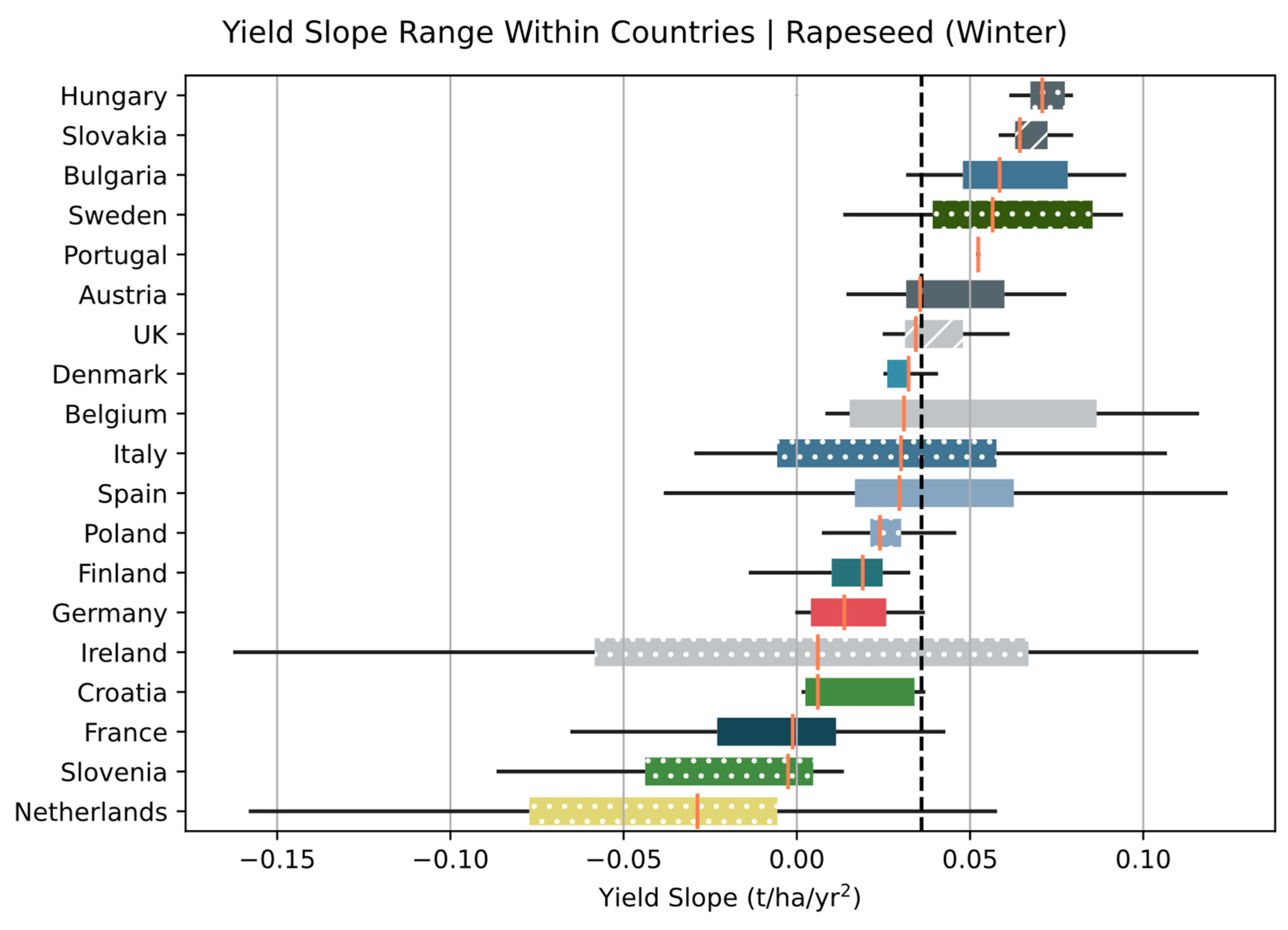
3.2.1. Yield Growth within Countries

Naturally, the spread in yield slopes observed at the scale of countries also manifests at the sub-national level for NUTS2 districts. Figure 8 and Figure 9 illustrate this district-level variation, by showing the range for all districts within a country, for winter wheat and rapeseed, respectively.

3.2.2. Variability and the “Additionality Ratchet”

Results such as the ones shown in Figure 8 and Figure 9 imply varying levels of tailwind and headwind additionality for projects in different parts of the same country, with larger differences possible in countries with wide “yield improvement gaps”. On the other hand, a country exhibiting a small yield improvement gap may do so for a number of reasons: because there are uniform yield trends throughout the country; because the crop in question is grown in a small area of the country; or because there is a low rate of data reporting.
We investigate variability at sub-national scales by calculating the “above-baseline” yield determined for each district, that is, the difference between the historically recorded yield and the baseline yield, which would be identified as additional by the low ILUC-risk methodology. Any significant amount of above-baseline production evident in these data would therefore indicate a limitation of the low ILUC-risk methodology, as it shows that non-additional material may be certified as additional.
Figure 10 and Figure 11 zoom into specific districts of two countries, to show the amount of above-baseline winter wheat that could be declared in each. The premise is that we consider a hypothetical typical farm in each district; this farm has a corresponding panel in the figures, indicated by the NUTS2 code in the legend. For the example under consideration, we say the farm gains low ILUC-risk certification in 2012; this means the initial point of its dynamic yield baseline is determined from records in the three-year period 2009–11. The baseline for each district is represented in the figures by straight dashed black lines spanning the ten years 2012–21; the actual data for the district are shown as solid, coloured lines, and the national average (for comparison) is the dotted coloured line in each district panel. Crop production above the baseline is shaded; this area represents the potential yield that could be spuriously certified as low ILUC-risk. The average above-baseline yield over the period is annotated in each panel.
Based on the recorded district-level data, our certified “farms” would have been able to declare a varying amount of above-baseline production as low ILUC-risk, though in reality no additionality measure was taken; all effects are purely based on business-as-usual background trends. The Hungarian case in Figure 11 shows large above-baseline gains, and, consulting Figure 5, we indeed see that Hungary has a history of high yield growth compared with the global average.
Inspection of the Austrian case in Figure 10 reveals a different phenomenon. Figure 5 shows that Austria’s national yield growth is similar to the global average, but we still see substantial amounts of material above the baseline. This is because the Commission’s methodology dictates that positive yield fluctuations are counted as additional, while negative yield fluctuations are bounded from below and are treated as zero additional material. This can be described as an “additionality ratchet”; a ratchet is a wheel designed to only turn in one direction, and here we see that additionality is only credited in one direction (i.e., above the baseline). This means that the running total of “additional” production—from fluctuations or otherwise—can only increase.
The new terms introduced in this paper to describe phenomena related to the RED II methodology are summarised in Figure 12.

3.2.3. Summary Statistics

Stepping back, we may characterise these trends at the EU scale, using the full dataset to determine how many districts could have declared spurious low ILUC-risk production, simply by following historical trends. As shown in Annex E of the Supplementary Material, a significant number of districts fall into this category; the European Commission will have to decide whether this is an acceptable outcome of its methodology.
Within these aggregate statistics, we can identify the districts for which the current definitions are the most advantageous, and which would be able to supply the greatest amount of spurious additional material. Figure 13 shows the district-level above-baseline yield calculated in 2018, assuming low ILUC-risk certification is successful in 2015. Each panel presents a different crop and indicates the proportion of districts which are above-baseline for that crop. Each bar represents a district, and bar styles correspond to the parent country in order to facilitate visual grouping of different districts into single countries.

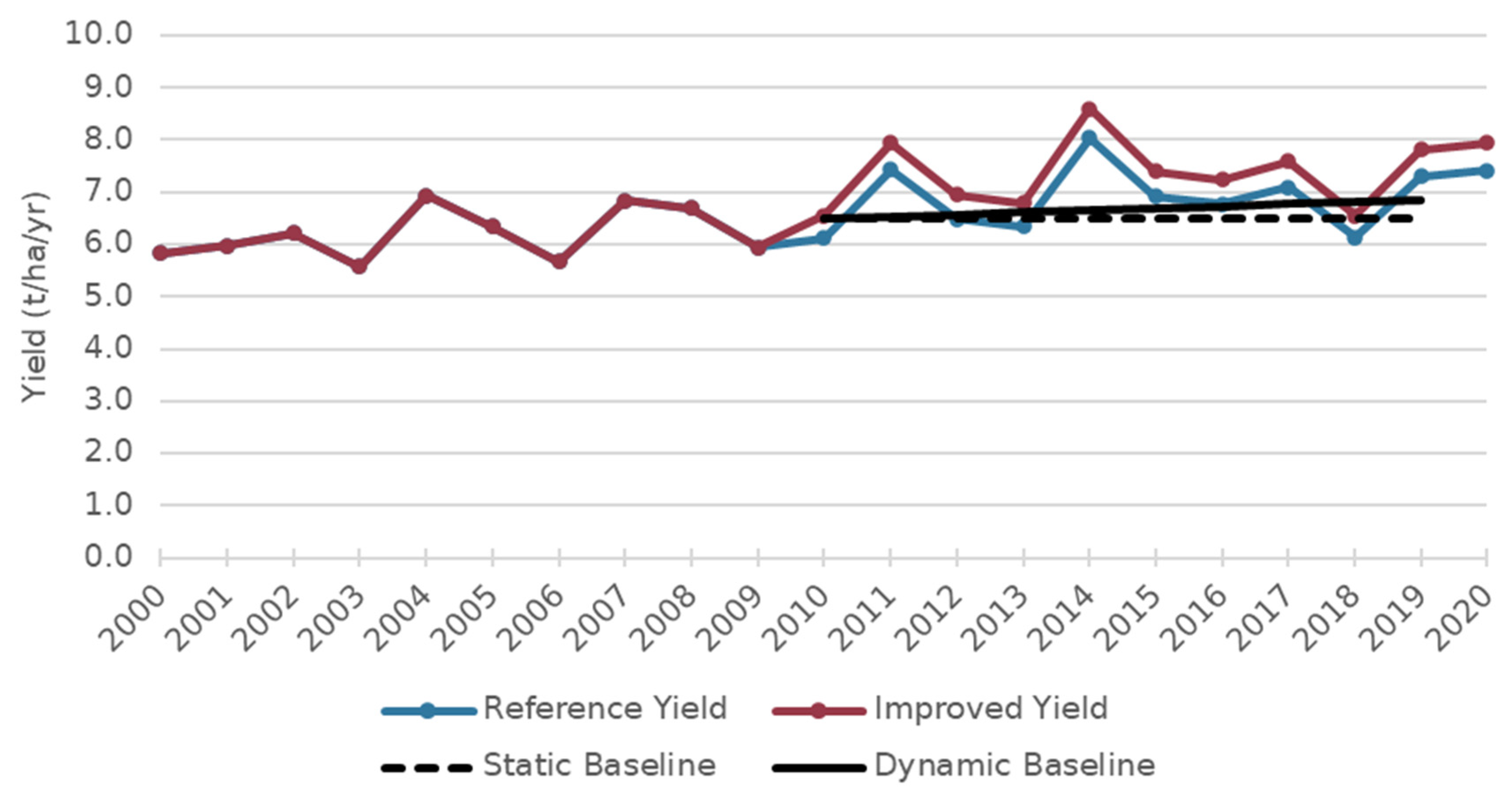
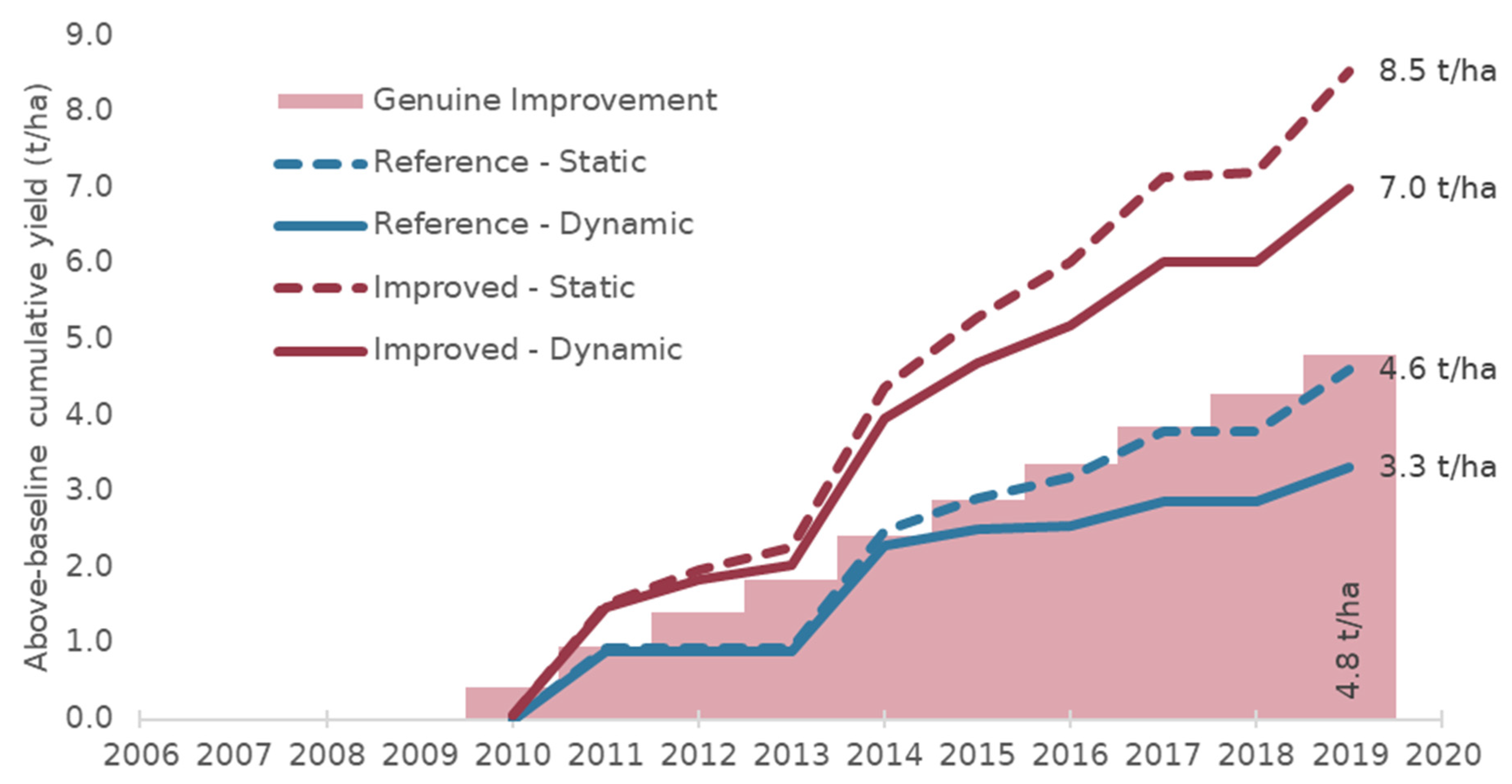
3.3. Static Yield Baselines

Constructing the dynamic yield baseline has been identified as a potential source of confusion, complication, and friction in deploying the low ILUC-risk system. Indeed, other low ILUC-risk frameworks beyond the one developed under the RED II ignore long-term productivity growth and treat the baseline as constant in time, for example, the International Civil Aviation Organisation’s Carbon Offsetting and Reduction Scheme for International Aviation (ICAO CORSIA) [15] and the existing framework under the Roundtable on Sustainable Biomaterials (RSB) [16]. This lowers the level of the baseline, and hence lowers the bar for producing low ILUC-risk feedstock, allowing more spurious material to be certified. In this section, we consider the impacts of using this kind of static yield baseline.

3.3.1. In Silico Experiment

The following analysis illustrates the magnitude of this effect by considering a hypothetical farm that implements a yield-improvement measure in pursuit of low ILUC-risk certification. In one scenario (the “reference scenario”), the measure has no effect, and yields track the historical recorded data with no improvement; in the other scenario (the “improved scenario”), the additionality measure has the effect of increasing yields by 7% compared to the reference scenario. While we—the authors and the readers of this study—know exactly what the impact of the additionality measure was (viz. 7%), a hypothetical observer who only has access to annual yield measurements from the field would have to apply the RED II methodology to these data in order to estimate the volume of additional material. By comparing this estimate with our perfect knowledge of the additional volume, we may investigate how the details of the methodology influences the quality of the estimate.
In principle, the comparison between the two baselines (static and dynamic) and the two scenarios (reference and improved) could be carried out for different choices of certification year, for any crop, and for any NUTS2 district. In the interests of brevity, for this analysis we have chosen 2010 as the year that the additionality measure is implemented, and low ILUC-risk certification awarded winter wheat as the crop, and AT31 (in Austria) as the district. The baselines start in 2010 at a value equal to the average of the yields in the three-year period 2007–09 and continue for a period of ten years. We assume that any yield improvement takes effect in the certification year onwards, which means that both the unimproved and the improved scenarios use the same yield values for initialisation.
Constructing these two baselines per district is sufficient to illustrate the issues at play; in particular, we note that, while Figure 5 shows Austria as a whole experiencing a mild headwind, the district under examination actually presents a tailwind. Since we are now focussing on a single district, we dispense with the country-specific colour coding that was used in previous figures.

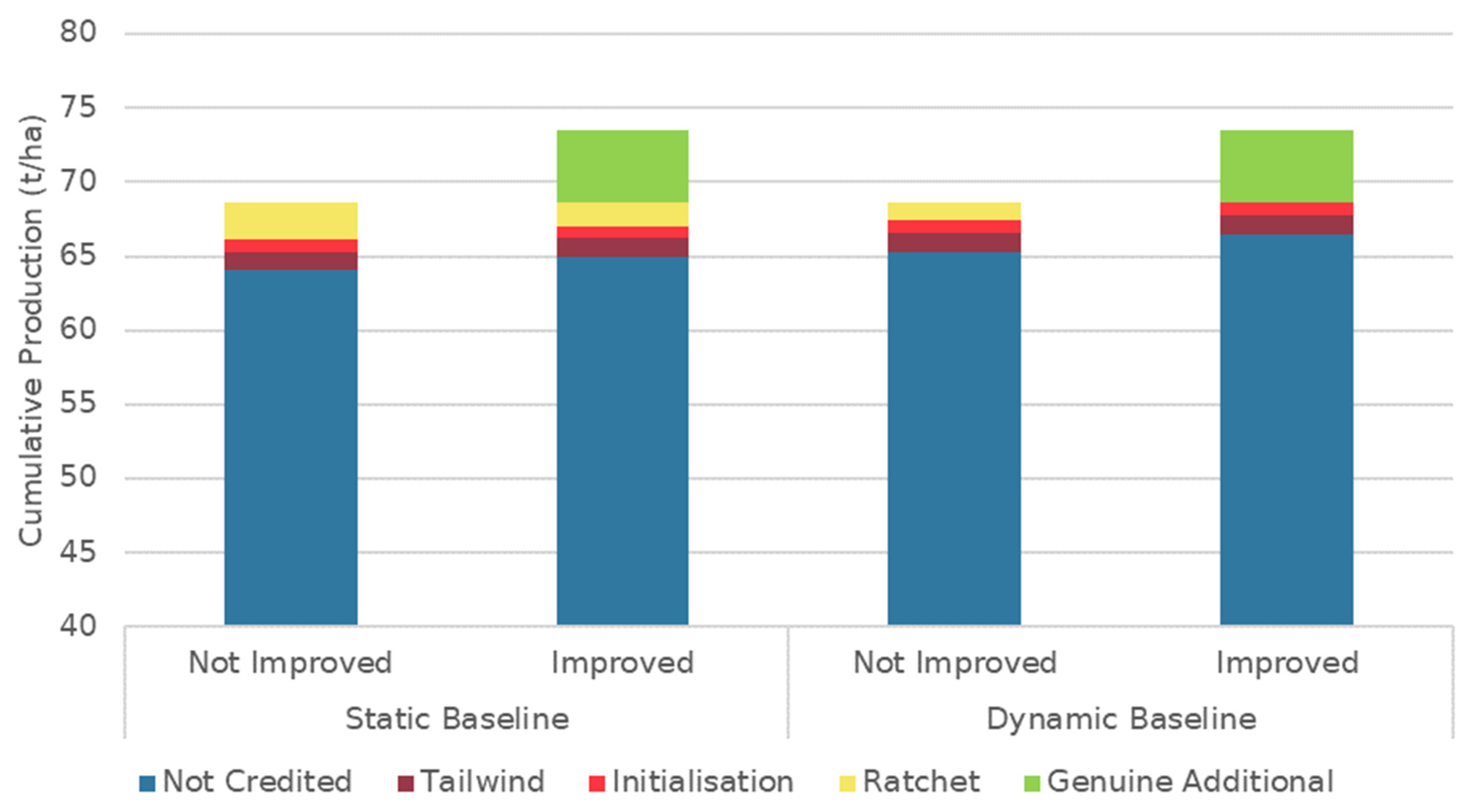
3.3.2. Spurious Additionality

Figure 14 introduces the yield data and the two baselines. The reference yield and improved yield are the same until the year 2010, when the additionality measure takes effect. After this, the improved yield is consistently higher by 7%, by construction. The cumulative “above-baseline” yield for the four cases is then shown in Figure 15 (lines), alongside the genuine additional yield (shaded area).
For the reference case in Figure 15 (two lower lines, blue), all production identified as above-baseline is in fact spurious, as the additionality measure had no effect. Unsurprisingly, the static baseline option gives a larger over-estimate of additionality than the dynamic baseline (+20–30%). As a side note, there is an apparent agreement between the genuinely additional yield boost in the improved case (shaded area) and the calculated above-baseline yield in the reference case, but this is a coincidence; it just so happens that a static baseline applied to data where no improvement has been made results in total spurious additional feedstock which is similar to the actual true additional material produced from a 7% yield boost. The match in no way supports the use of a static baseline.
In the improved case (two upper lines, red), the methodology is able to recognise that more feedstock is indeed being produced, but the calculated above-baseline production still substantially over-estimates the amount of additional feedstock shown by the shaded area: 25% and 40% of the “additional” material credited by the methodology is spurious, for the dynamic and static baselines, respectively.

3.3.3. Breakdown of Over-Crediting

Continuing the analysis of district AT31, Figure 16 presents a clear comparison of the total creditable additional production under the four cases considered. Everything above the dark blue bars is above the baseline and would be considered additional by the RED II methodology, but only the green component is genuinely additional. The spurious components are broken down into “tailwind” and “ratchet”—concepts which we have met before—and “initialisation” which is a further source of bias in the methodology, but which in the interests of brevity we have not discussed here.
In both the improved and the non-improved reference cases, a static baseline generates more above-baseline material than a dynamic baseline, as is expected. Moreover, the boost from using a static baseline tends to favour areas with low existing yields proportionately more than areas with high yields. This is because for higher-yielding regions, the difference between static and dynamic is a smaller fraction of the overall yield.
We can therefore think of a dynamic baseline as introducing some “drag” on the production of spurious additional material. This is especially pertinent for areas where there is high background yield growth, in the absence of any genuine or effective improvement measure. This drag operates indiscriminately in the sense that there are situations where a dynamic baseline would penalise areas which are legitimately producing additional material but are still failing to surpass the baseline (e.g., areas with strong headwinds). This would undermine the attractiveness of the low ILUC-risk system in these areas, and hence eliminate a potential route to investment in improved agricultural practices.

4. Discussion

The European Union’s “low ILUC-risk” system for biofuel certification allows economic actors in this sector to demonstrate that they have avoided the indirect land-use change (ILUC) impacts associated with growing crop-based biofuel feedstocks. The goal of this paper was to investigate the potential implications of how the rules for calculation of additional biomass production by yield improvement projects have been defined in policy. In particular, we have assessed provisions for calculating baseline yields; these are the baselines against which actual observed yields are to be compared when assessing the success of yield improvement measures undertaken by participating farms. The baselines thus determine the amount of agricultural production that can be certified for the market as low ILUC-risk.
The first step of this research was the creation of a cleaning pipeline for publicly available Eurostat data on crop productivity, covering countries in Europe at the national level and EU Member States at the scale of NUTS2 districts. We provide the final dataset and processing routine alongside this paper (see Annex B of the Supplementary Material) in the hope that it may be a useful starting point for other researchers or national agencies. This dataset then allowed us to quantify—at the NUTS2 district level—variability in crop yields and yield growth over time for a range of crops, including the cereal crops barley (summer and winter seasons), wheat (summer and winter seasons), durum wheat, maize, rye, sorghum, and triticale; the oil crops rapeseed (summer and winter seasons), sunflower seed, and soybean; and the sugar crop sugar beet.
On the basis of this, we were able to analyse potential weaknesses of the RED II low ILUC-risk methodology, whereby business-as-usual production of agricultural biomass could be wrongly classified as additional. The first of these potential weaknesses were termed “tailwind additionality” and “headwind additionality”. These effects are the result of background yield trends, which would make it easier or harder for projects to report production of additional biomass based on their geography, among other factors, rather than on the actual implementation or success of improved farm management practices. Were there to be widespread uptake of the low ILUC-risk concept, tailwind effects could tend to encourage the introduction of low ILUC-risk projects and cultivation of bioenergy feedstocks in areas where background yield growth is high. This would have the effect of allowing business-as-usual yield gains to be labelled as low ILUC-risk biomass and diverted into the bioenergy sector, undermining the goal of using certification to reduce ILUC emissions by identifying only additional biomass production. On the other side of the coin, headwinds would undermine the potential to use low ILUC-risk certification to support efforts to improve agricultural practices and productivity in areas where yield growth is low, as headwinds reduce the amount of truly additional biomass that could be detected and certified.
A second potential weakness of the RED II methodology was termed the “additionality ratchet”; this is where weather-driven annual yield fluctuations above the baseline are treated as additional, while fluctuations below the baseline are ignored. To illustrate, consider a low ILUC-risk project where the adopted yield increase measure fails for some reason; in principle this project should generate no creditable feedstock. However, the additionality ratchet guarantees that such a project will generate spurious additional material in every year in which the weather is favourable to the crop being grown, resulting in above-average yield.
These challenges speak to the tension between creating, on the one hand, robust rewards for genuinely additional production, and on the other, a practical system that can be applied on the ground by economic operators with limited visibility on their future yields. To its credit, the European Commission has established some guardrails. For example, an applicant for low ILUC-risk certification must submit their prediction of the yield improvement impact following the change in management practices on their fields (regardless of which types of crops are to be grown). Once certification has been granted and additional yields have been recorded, auditors are directed to refer back to this initial prediction and flag discrepancies of over 20% in the volume of additional biomass produced (which could arise from a strong tailwind). However, this is in itself a blunt instrument and there is no defined process to further investigate such a discrepancy, which may limit the utility of these checks.

Recommendations for Low ILUC-Risk Certification Systems

Based on our analysis, we offer the following recommendations for consideration in the development of systems for certifying low ILUC-risk biomass.
  • Yield improvement projections. Existing regulations require economic operators to estimate the impact of their additionality measures on future yields, which is a delicate task for which little to no guidance is provided. This imposes not only analytical burden, but also uncertainty on farmers and on auditors. The Commission could consider devising a template for forecasting, possibly with look-up tables, in collaboration with certification bodies.
  • More localised yield baseline slopes. Current regulations specify use of the global average yield trend for the slope of the dynamic yield baseline. The global average trend is a poor approximation to actual trend yields in many locations, and the use of a single slope of the dynamic yield baseline in all areas tends to exaggerate the systematic unfairness due to headwind and tailwind additionality. Adopting national or regional averages rather than global averages may give a more useful characterisation of what can be expected from business-as-usual yield development in a given location.
  • Surpassing yield predictions. At present, auditors must seek justification when operators’ production of additional biomass exceeds the predictions from the management plan by over 20%. What constitutes adequate justification is not precisely specified, nor does the Implementing Regulation specify what (if any) corrective actions should be taken on the part of the auditors if the justification given is inadequate or if the justification confirms that the material is not all additional (e.g., if the justification is that it was a good year for yields for all farms in the region). Without further specification this provision may have limited value in ensuring the integrity of the system; for instance, it does not actually control the benefits arising from tailwind additionality. It would be appropriate to review the application of this part of the rules, and to consider extending discretion to auditors to place some form of limit on the amount of biomass that is treated as additional when this threshold is passed.
  • Practice-based crediting. The aforementioned risk of certifying non-additional biomass due to tailwind additionality and the additionality ratchet has a flipside. This is that operators successfully applying additionality measures and delivering higher yields than would otherwise have been possible may yet find themselves unable to claim certifiable production due to adverse conditions in a given year or years. This uncertainty about rates of credit generation in the face of variability or of inauspicious background trends will reduce the value of low ILUC-risk certification as a driver of improved practices. One option that has been suggested in the past is to adopt a hybrid crediting scheme, under which some material would be certified as additional based on an auditor’s assessment that operators had appropriately applied additionality measures before consideration of the actual achieved annual yields.
  • Dynamic baseline. We have demonstrated in illustrative cases that the use of a dynamic baseline may reduce the extent to which non-additional material is certified. Operators of other systems (for example the system under CORSIA) could consider adopting a dynamic baseline approach.
  • Cleaned data. The agricultural data available from Eurostat are highly valuable to the research community, as well as to the officials of EU and national institutions. Provision of a better harmonised and cleaned dataset of crop yields and harvest areas would greatly facilitate research; we recommend that Eurostat consider creating such a dataset.

Supplementary Materials

The following supporting information can be downloaded at: https://www.mdpi.com/article/10.3390/app13106349/s1, Annex A: Data filtering and cleaning; Annex B: Cleaned dataset; Annex C: FAOstat crop yield slopes; Annex D: Country codes; Annex E: Above-baseline yield statistics; Annex F: Country-specific yield slopes.

Author Contributions

Conceptualisation: C.S., C.M. and C.P.; Methodology: C.S. and C.M.; Software: C.S.; Validation: C.S., C.M. and C.P.; Formal analysis: C.S.; Investigation: C.S.; Data curation: C.S.; Writing—Original Draft Preparation: C.S.; Writing—Review & Editing: C.M. and C.P.; Project administration: C.S. and C.P.; Funding acquisition: C.M. and C.P. All authors have read and agreed to the published version of the manuscript.

Funding

This research was funded by the European Commission Grant Agreement number 952872 (BIKE; https://www.bike-biofuels.eu/ (accessed on 11 May 2023)).

Institutional Review Board Statement

Not applicable.

Informed Consent Statement

Not applicable, as no personal data or experimental subjects were involved in the study.

Data Availability Statement

Data processing code and the key output dataset are included in the Supplementary Material.

Acknowledgments

The authors would like to thank Berien Elbersen and Simone Verzandvoort for early discussions as part of the BIKE project.

Conflicts of Interest

The authors declare no conflict of interest.

References

  1. Daioglou, V.; Woltjer, G.; Strengers, B.; Elbersen, B.; Barberena Ibañez, G.; Sánchez Gonzalez, D.; Gil Barno, J.; van Vuuren, D.P. Progress and Barriers in Understanding and Preventing Indirect Land-Use Change. Biofuels Bioprod. Biorefining 2020, 14, 924–934. [Google Scholar] [CrossRef]
  2. Malins, C.; Searle, S.; Baral, A. A Guide for the Perplexed to the Indirect Effects of Biofuels Production; ICCT: Washington, DC, USA, 2014; pp. 1–166. [Google Scholar]
  3. Searchinger, T.; Heimlich, R.; Houghton, R.A.; Dong, F.; Elobeid, A.; Fabiosa, J.; Tokgoz, S.; Hayes, D.; Yu, T.H. Use of U.S. Croplands for Biofuels Increases Greenhouse Gases through Emissions from Land-Use Change. Science 2008, 319, 1238–1240. [Google Scholar] [CrossRef] [PubMed]
  4. Plevin, R.J.; Jones, J.; Kyle, P.; Levy, A.W.; Shell, M.J.; Tanner, D.J. Choices in Land Representation Materially Affect Modeled Biofuel Carbon Intensity Estimates. J. Clean. Prod. 2022, 349, 131477. [Google Scholar] [CrossRef]
  5. Wicke, B.; Brinkman, M.L.J.; Gerssen-gondelach, S.J.; van der Laan, C.; Faaij, A.P. ILUC Prevention Strategies for Sustainable Biofuels: Synthesis Report; Copernicus Institute of Sustainable Development, Utrecht University: Utrecht, The Netherlands, 2015. [Google Scholar]
  6. European Parliament and European Council Directive (EU) 2018/2001 of the European Parliament and of the Council on the Promotion of the Use of Energy from Renewable Sources. Off. J. Eur. Union 2018, 328, 82–209.
  7. Malins, C. Risk Management: Identifying High and Low ILUC-Risk Biofuels under the Recast Renewable Energy Directive; Cerulogy: London, UK, 2019. [Google Scholar]
  8. Searle, S.; Jacopo, G. Analysis of High and Low Indirect Land-Use Change Definitions in European Union Renewable Fuel Policy; ICCT: Washington, DC, USA, 2018; p. 26. [Google Scholar]
  9. European Commission Delegated Regulation (EU) 2019/807. Off. J. Eur. Union 2019, L133/1, 1–7.
  10. Peters, D.; Hähl, T.; Kühner, A.K.; Cuijpers, M.; Stomph, T.J.; van der Werf, W.; Grass, M. Methodologies for the Identification and Certification of Low ILUC Risk Biofuels; Ecofys: Utrecht, The Netherlands, 2016. [Google Scholar]
  11. Dehue, B.; Meyer, S.; van de Staaij, J. Responsible Cultivation Areas Identification and Certification of Feedstock Production with a Low Risk of Indirect Effects; Ecofys: Utrecht, The Netherlands, 2010. [Google Scholar]
  12. Sumfleth, B.; Majer, S.; Thrän, D. Recent Developments in Low ILUC Policies and Certification in the EU Biobased Economy. Sustainability 2020, 12, 8147. [Google Scholar] [CrossRef]
  13. Panoutsou, C.; Giarola, S.; Ibrahim, D.; Verzandvoort, S.; Elbersen, B.; Sandford, C.; Malins, C.; Politi, M.; Vourliotakis, G.; Zita, V.E.; et al. Opportunities for Low Indirect Land Use Biomass for Biofuels in Europe. Appl. Sci. 2022, 12, 4623. [Google Scholar] [CrossRef]
  14. European Commission Implementing Regulation (EU) 2022/996. Off. J. Eur. Union 2022, L168, 1–62.
  15. ICAO. CORSIA Methodology for Calculating Actual Life Cycle Emissions Values, 3rd ed.; ICAO: Montreal, QC, USA, 2022. [Google Scholar]
  16. Roundtable for Sustainable Biomaterials. In Low ILUC Risk Biomass Criteria and Compliance Indicators Low ILUC Risk Biomass Criteria and Compliance Indicators; Version 0.3; Roundtable on Sustainable Biomaterials: Geneva, Switzerland, 2015.
Figure 1. Sketch of the key steps for low ILUC-risk certification applicants; the focus of this paper is highlighted.
Applsci 13 06349 g001
Figure 2. Crops considered in this study.
Applsci 13 06349 g002
Figure 3. Processing pipeline for the Eurostat dataset.
Applsci 13 06349 g003
Figure 5. Yield slope per country for winter wheat (left) and sunflower seed (right), with FAOstat global average indicated as a vertical dashed line. Note that in Figure 5 and subsequent figures, countries which share the same colour are distinguished from each other by an overlaid pattern. See for instance the light grey bars for Ireland, UK, and Belgium towards the bottom of the left panel of Figure 5.
Applsci 13 06349 g005
Figure 6. Yield slopes per country (dots) for cereal crops, with the FAOstat global average indicated for each. Note that countries are labelled by the two-letter country code; see Annex D of the Supplementary Material.
Applsci 13 06349 g006
Figure 7. Yield slopes per country (dots) for oil crops, with the FAOstat global average indicated for each.
Applsci 13 06349 g007
Figure 8. Yield slopes of winter wheat, for districts within each country. Note that this is a standard box-and-whisker plot. For each country, it indicates the median among districts (vertical orange lines), quartiles (coloured boxes), and range (whiskers). The global average yield slope is marked for reference (vertical dashed line). Here and in plots that follow, we eliminate districts with very small land area dedicated to a crop, as these may unduly skew the statistics.
Applsci 13 06349 g008
Figure 9. Yield slopes of rapeseed, for districts within each country. See the note below Figure 8 for more description.
Applsci 13 06349 g009
Figure 10. Above-baseline production for hypothetical Austrian low ILUC-risk projects which grow winter wheat and gain certification in 2012; the yield patterns are assumed to follow the district average. Note that each panel in this figure corresponds to a different NUTS2 district within Austria (AT); the district ID is indicated in the panel legend, along with the average above-baseline production in parentheses. For each district, three quantities are plotted: the district’s annual historical yield (solid line); the national historical yield (dotted line—these values are the same in each panel); and the calculated dynamic yield baseline for the district (black dashed line). Units are t/ha/yr.
Applsci 13 06349 g010
Figure 11. Above-baseline production for hypothetical Hungarian low ILUC-risk projects which grow winter wheat and gain certification in 2012; the yield patterns are assumed to follow the district average. See the caption for Figure 10 for further elaboration.
Applsci 13 06349 g011
Figure 12. Summary of new terms developed in this study.
Applsci 13 06349 g012
Figure 13. District-wise above-baseline yield for cereal crops in 2018, assuming low ILUC-risk certification in 2015, one column per district. Note that while each column corresponds to a NUTS2 district, the number of district labels on the x-axis has been reduced for visibility. Only districts with positive above-baseline yield are shown; the number of such districts as a fraction of the total in the dataset is indicated as an annotation in each panel.
Applsci 13 06349 g013
Figure 14. Yield data for winter wheat in district AT31, showing the two baseline options in black.
Applsci 13 06349 g014
Figure 15. Cumulative above-baseline yield (growing over 10 years), starting in the certification year. Note that the cumulative total at the end of the certification period is annotated for each case. The genuinely additional cumulative production is indicated in the lower-right and is rotated for distinction.
Applsci 13 06349 g015
Figure 16. Total additional yield of winter wheat in district AT31 (Austria) over the ten-year certification period, split into genuine and spurious improvement. Note that the vertical axis starts above zero in order to magnify the above-baseline portion.
Applsci 13 06349 g016
Disclaimer/Publisher’s Note: The statements, opinions and data contained in all publications are solely those of the individual author(s) and contributor(s) and not of MDPI and/or the editor(s). MDPI and/or the editor(s) disclaim responsibility for any injury to people or property resulting from any ideas, methods, instructions or products referred to in the content.

