Article

3D Structural Topology Optimization Using ESO, SESO and SERA: Comparison and an Extension to Flexible Mechanisms

by
Hélio Luiz Simonetti
1,*,
Valério S. Almeida
2,
Francisco de Assis das Neves
3,
Virgil Del Duca Almeida
4 and
Marlan D. S. Cutrim
5
1
Department of Mathematics, Federal Institute of Minas Gerais (IFMG), Betim 32677-764, MG, Brazil
2
Department of Geotechnical and Structural Engineering, The School of Engineering of the University of São Paulo (EPUSP), São Paulo 05508-010, SP, Brazil
3
Department of Civil Engineering, Federal University of Ouro Preto (UFOP), Ouro Preto 35400-000, MG, Brazil
4
Department of Automation and Control Engineering, Federal Institute of Minas Gerais (IFMG), Betim 32677-764, MG, Brazil
5
Department of Structure Engineering, Geotechnics of the Polytechnic School, The University of São Paulo (USP), São Paulo 05508-010, SP, Brazil
*
Author to whom correspondence should be addressed.
Appl. Sci. 2023, 13(10), 6215; https://doi.org/10.3390/app13106215
Submission received: 24 January 2023 / Revised: 16 February 2023 / Accepted: 7 March 2023 / Published: 19 May 2023

Abstract

:
This article investigates the study of Topology Optimization (TO) in 3D elasticity problems to determine the optimal topology by applying the evolutionary methods of Smoothing Evolutionary Structural Optimization (SESO), Sequential Element Rejection and Admission (SERA), and Evolutionary Structural Optimization (ESO). These procedures were implemented in MATLAB code as an extension of Top3d implemented for SIMP by using the eight-node hexahedral finite element formulation in three-dimensional elastostatic structures. The approaches conducted in the present study are demonstrated with numerical examples involving the compliance minimization criterion. Further, a brief synthesis of flexible mechanisms was studied to emphasize the performance of complaint mechanisms measured in terms of two design specifications/functionalities: mechanical and geometrical advantages, which are the highlights of this article. To show the gains of the proposed methods, numerical results obtained are compared with Solid Isotropic Material with Penalization (SIMP) models.

1. Introduction

As its main objective, structural optimization has the best distribution of materials in the solution domain. Researchers have investigated this topic for 2D elastic analysis in high-level programming languages, such as MATLAB or Python, because of easier implementation and post-processing analysis. For example, the pioneering work of Sigmund [1] presented a code with 99 lines by using the Solid Isotropic Material with Penalization (SIMP) method. In addition, as an extension of [1] and considering a density filter scheme, 88 lines achieved more computational efficiency [2]. Different methods have been explored in this sense, such as a compact implementation of the Level Set method (LSM) for statically loaded structures, where the minimization of compliance for a 2D linear elastic analysis was modeled [3]. The Bi-Evolutionary Structural Optimization (BESO) model was developed by [4] using the objective function of compliance minimization. It is also an extension of the code presented in [3]. In the work of [5], the code written in MATLAB for topology optimization of structures and compliant mechanisms was developed and implemented in the Sequential Element Rejection and Admission (SERA). This included sensitivity analysis and a mesh-independency filter.
In the sense of 3D topology optimization elastic problems, many solutions have been proposed using MATLAB code and the SIMP method, such as [6], which investigated a stress-based topology optimization mathematical model, or [7], which considered multiple load cases. Additionally, some works generated suitable outputs for additive manufacturing [8,9]. Large-scale topology optimization problems have been previously discussed by [10], which showed a parallel computing paradigm added to domain decomposition and a preconditioned conjugate gradient algorithm applied to solve equilibrium equations. Moreover, optimization was solved using sequential convex programming. A 100-line code using Python language was presented by [11], where general 3D topology optimization problems were solved via compliance minimization and with a volume constraint using the BESO method in multiple load cases and nonlinearities models. In [12], a TO formulation, including simplified additive manufacturing (AM), was presented. The procedure involved compliance minimization, eigenfrequency maximization, and compliant mechanism design.
Recent research has proposed the application of deep learning-based paradigms in TO models. For instance, Ref. [13] explored the use of a framework by training data to accelerate the convergence of the final required optimal topology, mapping out the design variables and their respective sensitivities. Moreover, Ref. [14] were the first to apply the deep reinforcement learning agent concept to optimize 2D topologies and discretized problems solved via a classical gradient-based TO. Additionally, Ref. [15] proposed the use of a convolutional neural network in the deep-learning model to maximize, via data-driven models, the bulk modulus and shear modulus in metamaterial design systems.
This article investigates the application of SESO (originally proposed by [16]), the application of classical ESO (originally proposed by [17] and reviewed by [18]), and the application of SERA evolutionary methods. The main novelty of the paper is the extension of SESO and ESO (in MATLAB code) to a 3D TO using the minimization of compliance growth for solving flexible mechanisms, as it has only been previously evaluated using the SERA method [19]. Additional novelties in the present study include the extension of the SERA method for 3D TO problems with several load cases in flexible mechanisms and in structures with cavities. Furthermore, the final secondary novelty is the implementation of the conjugate gradient method using the Jacobi preconditioner in all the present formulations for accelerating the linear solver algorithm.
The remainder of the article is organized as follows: Section 2 presents the definition of the minimum compliance problem for the different optimization methods implemented in this article; Section 3 presents the influence of certain parameters in the optimization procedures, comparing ESO, SERA, SESO, and SIMP; Section 4 briefly describes compliant mechanism synthesis; Section 5 presents numerical examples; and Section 6 offers conclusions.

2. Optimization Problem Formulation

2.1. Problem Statement–Minimum Compliance

The topological optimization (TO) problem can be defined as a binary problem whose the objective is to provide the best material distribution in the solution domain, according to the specified criteria. The TO problem analyzed herein is the classical formulation for compliance, which minimizes the work done by external forces subject to a desired pre-scribed volume, V*. The mathematical formulation of this problem may be expressed as
M i n i m i z e     C x = F T u x = i n u i T K i x i u i s u b j e c t   t o :   V x = 1 i = n x i p V i V *    
where compliance C x is the objective function ;     F   and u   are the global force and generalized displacement vectors, respectively; K   is the global stiffness matrix; V x is the total volume of the structure; V i is the volume of the element at each iteration; V* is the prescribed final limit volume ;   x i   is the artificial density of the element; and n is the total number of elements.
The evolutionary structural optimization methods are based on a simple and empirical concept that a structure evolves to an optimal, slowly removing the elements with lower desired sensibility. To maximize the structure’s stiffness, compliance minimization has replaced the stress criterion, as described in Equation (1). Thus, it can be highlighted that in the ESO, SESO, and SERA methods, the material is added and removed from the design domain until an optimal setting is reached. Therefore, they are bidirectional in nature. The major difference between them is the heuristic of removal and adding elements from the structure domain. The SERA method applies two separate criteria for removing and adding elements from the domain, allowing the status change from “passive” to “active” and vice versa. In this way, the final topology is constructed with all real materials present in the structure. For more details about the SERA method, see [5,16].
The SESO method uses only one criterion to perform this procedure, the elements that attend this criterion are removed from the design domain, ordered, grouped, and p% of the groups with lower compliance are discarded and (1 − p%) are returned to the structure, smoothing the “hard-kill” procedure used in ESO, i.e., the total removal of the elements that meet the rejection criterion. In addition, discrete variables ensure that the final topology is free of gray regions, as in continuous methods, such as the SIMP. It’s important to point out that SESO and ESO use domain elements as their discrete variables, while SERA [5,19] and SIMP [1,2] use element density instead.
It is noteworthy that, in the formulation described in Equation (1), the artificial density of the element   x i     is the design variable of all methods, which is computed as follows:
E S O x i = 1   a c t i v e   e l e m e n t   x i = x m i n   i n a c t i v e   e l e m e n t S E S O : x i = 1   a c t i v e   e l e m e n t x i = x m i n   i n a c t i v e   e l e m e n t x i = η i     a c t i v e   e l e m e n t S E R A : x i =   x m i n , 1 S I M P : x m i n < x i < 1
considering x m i n = 1 E 9 ,   η i   being a weighted function, 0 η i 1 , presented in [13]. The stiffness matrix is updated as presented in the item 2.2 and p is the penalization factor, with p = 1 being considered to ESO, SESO and SERA methods and p = 1, 2, …, p m a x ( p m a x > 3 ) for SIMP [1,2].
The way as all the aforementioned methods evaluate the artificial density parameter is defined by the desired objective function by computing the elemental sensibility, which is iteratively applied to remove or keep the element in the design domain. Some methods, such as the SERA [5,19] or the variant of ESO, BESO [4], can reintroduce elements into the actual design domain, from which the procedure of creating cavities is applied until the criterion is reached.
Using the Optimality Criteria (OC) method and the strategy suggested by [20], the design variables were updated. According to the OC formulation, when the constraint is inactive, convergence will be achieved if the Karush–Kuhn–Tucker (KKT) conditions are met.

2.2. Sensitivity Analysis

There are several methods to obtain the sensitivity of the design variables, such as those pointed out by [6,7,18]. Thus, without changing its removal heuristic, according to [13], it can be expressed as follows:
E i x = E m i n + x i p E 0 E m i n
with E m i n being the modulus of elasticity for the “empty” material, the value E m i n = 10 9 used to avoid the singularity in the stiffness matrix, K x , E 0   is the modulus of elasticity for the “solid” material. Therefore, the stiffness matrix using Equation (3) can be written as
K x = i = 1 n E m i n + x i p E 0 E m i n k i 0
Deriving the equilibrium equation K x u x = F and making some mathematical manipulations:
u x x i = K 1 x K x x i u x
The derivative of the objective function, Equation (1), in relation to x i , after applying Equation (5) and using the expression F T = u T x K x , we obtain, which is given by
C x x i = u T x K x x i u x
Substituting the derivative of Equation (4) in relation to xi in Equation (6), the sensitivity of the objective function can be rewritten as follows:
C x x i = u T x p x i p 1 E 0 E m i n k i 0 u x
The sensitivity of the cost function with respect to the design variables, Equation (7), is obtained using the finite difference method. The sensitivity expression is valid for the four methods described in this paper. However, with different physical interpretations since SIMP and SERA have the element density as a design variable, while ESO and SESO use the domain element instead.

3. Comparing SESO and SERA with Other Topology Optimization Methods

Currently, the SIMP method is the most used for TO and has shown its effectiveness in structural engineering applications. The SESO, SERA, and ESO methods implemented in this article use the same eight-node hexahedral finite element proposed by [7]. Consequently, the findings of SESO, SERA, and ESO are compared with Top3d by [7], which make use of SIMP. Issues such as checkerboard, local optimal, and mesh dependence arise with evolutionary optimization models, according to [21]. By using this heuristic filtering scheme to address numerical instabilities in TO, a comparison can be made between two levels: with and without a mesh independence filter.
Mathematically, the spatial filter is an additional constraint inserted into the optimization problem as a way of smoothing out the spatial distribution of the design variables in the solution domain, minimizing the mesh dependence, and controlling the topology complexity. Thus, with an increase in the radius value, gradients are restricted to smaller values and the transition between solid (material) and empty (without material) becomes smoother, generating more intermediate compliance elements. Given that the OT procedure is affected by the radius of the filter, particularly when it is larger, the optimization problem would not have a solution using the initial condition proposed, as the gradients of the design variables would be restricted to very low rates of variation. Thus, a simple function for the density filter can be written as follows:
x ¯ i = j = 1 n H i j v j x j j = 1 N H i j v j
where the element x i   with volume v i , x ¯ i is the weighted average of the distances from the centers of the neighboring elements x i within a sphere of radius R with H i j its weighting factor defined as follows:
H i j = R d i j
with R being the radius, see Figure 1, of the sphere centered on the element x i and d i j   is the distance between the centers of the elements x i and x j given by:
d i j = ( x i x j ) 2 + ( y i y j ) 2 + ( z i z j ) 2
where x i , y i , z i and x j , y j , z j are, respectively, the coordinates of the centers of the elements i and j.
The filtered element is incorporated into the optimization procedure, and the modulus of elasticity of the modified SIMP method is given by:
E i x ¯ = E m i n +     x i ¯ p E 0 E m i n ,   x i ¯ 0 , 1
Thus, it is possible to determine the sensitivity of the x ¯ i (filtered) elements of the SESO, SERA, and ESO methods which given by the expression:
E i x ¯ = E m i n +     x i ¯ E 0 E m i n ,   x i ¯ 0 , 1
Therefore, SESO, SERA, and ESO have the sensitivity at the level of the filtered elements given by:
C x i ¯ x i = u i T x i ¯ E 0 E m i n K i 0 u i x i ¯
where u is the nodal vector of the elements’ displacements and K i 0 is the stiffness matrix of the element. For the SIMP method:
C x i ¯ x i = u i T x i ¯ p x i ¯ p 1 E 0 E m i n K i 0 u i x i ¯
The algorithm of the optimization methods can be described as follows:
Step 1:
Discretize the domain using a refined finite element mesh;
Step 2:
Specific the maximum final volume (V*) and the parameters for the desired method. ESO and SESO: rejection rate (RR), evolutionary rate (ER) and the weighted function (η). SERA: total number of iterations (Ntot), progression rate (PR) and smoothing ratio (SR). SIMP: p and   x m i n
Step 3:
Solve the linear elastic problem, applying boundary conditions;
Step 4:
Calculate the value of the compliance sensitivity value of each element and update the ratios or thresholds for the method;
Step 5:
Remove or introduce elements with the lowest (highest) sensitivity number;
Step 6:
Repeat Steps 3 to 5 until the prescribed limit volume has been reached.

3.1. Comparing Topology Optimization Algorithms with a Mesh-Independency Filter

A long cantilever, Figure 2, is selected as a test example. It involves a series of broken bars during the optimization procedure. A concentrated load of F = 1 KN is applied in the middle of the free edge. The cantilever has dimensions L = 160, h = 40 and b = 4. Young’s modulus E = 1 MPa and Poisson’s coefficient 0.30 . The design domain was discretized with a fine mesh of 160 × 40 × 4 ,   totaling 25,600 cubic elements of eight nodes, and the volume constraint for this structure is 0.30 of the initial volume. Table 1 shows the optimization parameters used in the four methods presented. Using the filter, it is noted that the topologies obtained with the SESO, SERA, and ESO methods are similar since the topology achieved with the SIMP method is quite different. It is noteworthy that the ESO and SESO methods obtained equal compliances, with a lower value than the SERA, which computationally, for this problem, proved to be more efficient.
In most cases, discrete evolutionary methods, when using a small evolutionary ratio (ER) and a finer mesh, reach optimal settings in the solution domain. This is one of the advantages of these methods. However, its computational efficiency is extremely dependent on the selected parameters, such as its mesh and ER parameter. Compared to these methods, the modified SIMP is more stable and less dependent on optimization parameters provided that exponent p of the penalty is correctly calibrated; in this article, p = 3. This method will produce optimal solutions because the optimization criteria are met. The optimum solution presented by SIMP has approximately 41.5% greater compliance, and the manufacture of the resulting structure is more difficult.

3.2. Comparing Topology Optimization Algorithms without a Mesh-Independency Filter

The problem above is analyzed again using the same mesh, but now without using the mesh independence filter. Table 2 lists the parameters and solutions obtained. It is highlighted that SESO and ESO are similar in their structural design and the final values of the objective function. This is not surprising, as the evolutionary procedure for these methods uses the same removal heuristic. However, SESO is a bidirectional method; that is, it has a “soft-kill” removal. It allows adding elements during the evolutionary process, and ESO is unidirectional because it has its most radical “hard-kill” removal. The SERA and SIMP methods have a density as the design variables. These methods showed a higher concentration of zones with checkerboard patterns and optimal settings quite different from those presented by ESO and SESO methods. As the SIMP has a penalty factor p = 3 and the central element is not filtered, the sensitivity of the stiffness of this element increases proportionally to the triple of the square of its density, justifying this concentration, i.e., the sensitivity is given by Equation (14). Replacing the value of p = 3 in this equation results in the proportionality factor of 3 x ¯ i 2 , where x i is the density of the element.
In a refined mesh, the number of finite elements within the radius increases, providing greater control over the region. Thus, it is possible to smooth out large variations in the objective function (compliance); that is, the peaks in the objective function can be controlled by the filter. In addition, the filter has the ability to control topology complexity. The absence of the filter allows the appearance of checkerboard formations (regions where compliance is high).

4. Compliant Mechanism Synthesis

Topology optimization of a compliant mechanism by the evolutionary structural optimization procedures ESO, SESO, SERA, and SIMP are presented here. In [22] defines a compliant mechanism as a morphing structure that undergoes elastic deformation to transform force, displacement, or energy. A typical goal of a compliant mechanism design is to maximize certain displacements. Another different way of expressing the problem is with the mechanical advantage objective function, where the design purpose is to maximize the output force for a given input force. Herein, the optimization problem in terms of maximum output displacement is given by:
M i n i m i z e   C   x = u o u t ( x ) T = L T U x   s u b j e c t   t o   V x = x T V V * < 0 x Ψ ,   Ψ = x R n / 0 x 1
L is a unit length vector with zeros at all degrees of freedom except at the output point where it is unity, and U x = [ K x ] 1 F . The sensitivity of the cost function obtained from Equation (4) is given by:
K x U d x = L
where it is defined a global adjoint vector U d x from the solution of the adjoint problem. Therefore, the objective function is expressed as follows:
C x = U d ( x ) T K x U d x
where the vector U d is the dummy load–displacement field, and the vector U is the input load displacement.
The new design variable will be updated by the derivative of the objective function that represents the sensitivity of the element and is given by Equation (18):
C x i ¯ x i = u d i T ( x ) T x i E 0 E m i n k i 0 u i x i

5. Numerical Example

The following examples focus on TO based on minimizing compliance. The geometry and boundary conditions for numerical applications are represented in each case. All numerical examples were processed on a Core i7-2370, 8th Gen notebook, 2.8 GHz CPU with 20.0 GB (RAM).

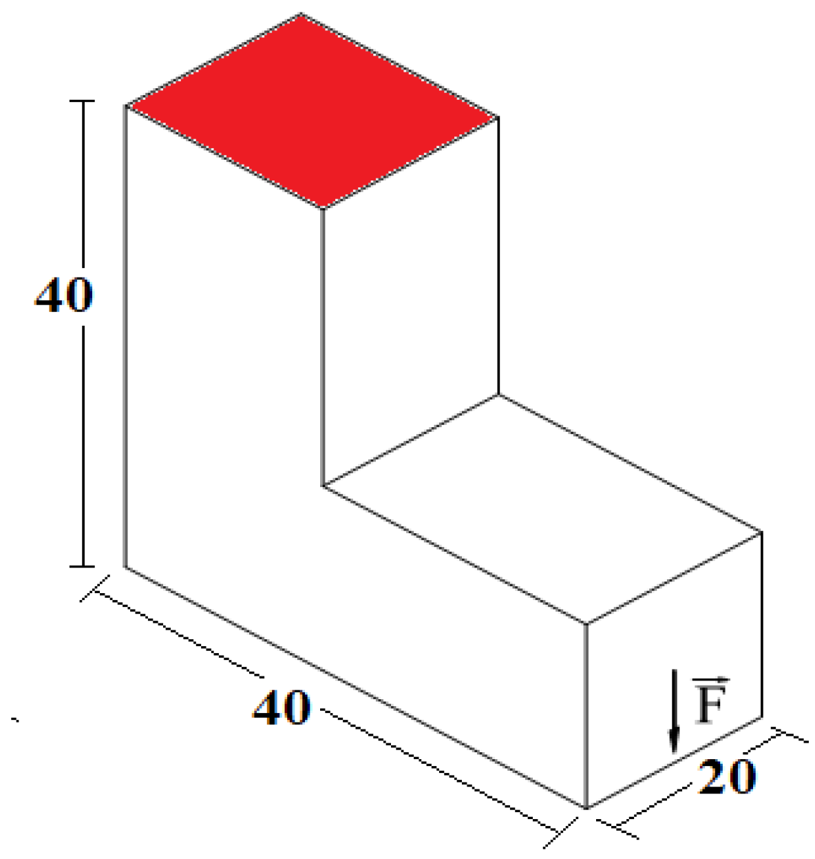
5.1. Example 1—L-Shaped Beam Problem

In this section, an L-shaped structure is investigated, as shown in Figure 3, where the red area represents the restricted displacements. To simulate the L-shaped structure, a rectangular design domain is defined, using a fine mesh of 40 × 40 × 20 hexahedral finite elements with dimensions equal to 1mm, producing a total of 32,000 finite elements, and certain elements in the domain are forced to be in the lower limits of the density values ( ρ i = 10 9 ) for SERA and SIMP, while SESO and ESO have their limit values of the elements ( x i = 10 9 ). The minimum radius is equal to 1.2   mm . Table 3 shows the optimization parameters, the number of iterations, the objective function, and the computational cost of each method for the problem of an L-shaped structure. Figure 4 shows the cross-section, quota z = 10   mm , of the optimal settings of the L-shaped structures presented in Figure 4. It was observed that the place where the force is applied has relatively higher values of compliance, and the methods SESO, ESO, and SIMP keep a larger amount of material close to this region. In contrast, the SERA method can remove more material. This can be explained by the fact that the method has a heuristic of inserting virtual elements in regions where compliance is high. Additionally, on the internal surface of Figure 4, at the edge where the structure forms an angle of 90°, compliance has high values, also requiring more material in this corner region. Figure 5d shows that the SIMP model needs more material in the corner region, where the structure has bending stress, unlike the discrete models that managed to keep the structure’s stiffness by removing material in this region, supporting these stresses with two bars as can be seen in Figure 5a–c.

5.2. Example 2—A Channel Beam

Figure 6 shows a U-shaped structure, fixed at both ends, with an initial thickness of 0.5 m. The elasticity module of the material is E = 210 GPa, and Poisson’s ratio ν = 0.30 is assumed. It is considered a combination of gravitational and external loads, with a density of ρ = 2700   kg / m ³ and a distributed load of intensity q = 0.094 MPa. The domain was discretized with a 90 × 18 × 18 mesh, and the constraint volume equals V = 13.5 m3. Figure 7 shows the optimal setting in the form of an arched bridge with hangers. The optimal topologies are shown in Figure 7. It is evident that an arch profile with fairly uniform thickness is generated above the deck. The four topologies are similar because the combined load requires more materials in the arc to support heavier loads. If a fine mesh was used, the arc profile could be smoother. However, there is a great similarity between the optimal topologies and the real arch bridges. This means that the optimization process is valid. It should be noted that the structural design using the SERA method added material at the top, bracing the two arches. The SESO, SERA, ESO, and SIMP methods effectively find optimal solutions to problems that include the combined use of gravity loading and external forces. Additionally, SERA reached the lowest value for the objective function, approximately C = 1186.87   Nm , 3.4% in relation to the SESO and ESO methods and 41% in relation to the SIMP.
The compliances of solutions SESO, SERA, and ESO are very close. However, with p = 3 , the SIMP method converges to a great location with higher compliance. Figure 8 shows the evolution history of the objective function using the four topology optimization methods. Compliance for the SESO, SERA, and ESO methods increases with small jumps (due to the formation of hangers on the structure) as the total volume gradually decreases. After reaching the prescribed volume, in subsequent iterations, while the volume remains unchanged, compliance gradually converges to a constant value. Unlike SESO, SERA, and ESO, the SIMP method has the volume restriction met throughout the iterative procedure. Thus, the volume remains constant, and compliance gradually decreases until the convergence criterion is reached.

5.3. Example 3—Compliant Mechanism–Mechanical Advantage and Geometrical Advantage

Flexible mechanisms are jointless mechanisms that use elastic deformation as a source of motion. Therefore, in the elastic deformation of the structure of a flexible mechanism, energy is absorbed and can no longer be considered conserved between the input and output ports. Thus, the elastic deformation changes the kinematic characteristics and the optimal solution [23]. In rigid-body mechanisms, Mechanical Advantage (MA) is entirely decided by kinematics. In compliant mechanisms, kinematics, forces, and elastic deformation contribute to MA. Therefore, the main tasks that the designer must associate with the optimization topology of flexible mechanisms are flexibility, stiffness, and efficiency.
According to [24], it can be stated that the problem formulation, in which the mechanical advantage (MA) and the geometric advantage (GA) are placed as an objective function for SESO, is given by Equation (19):
M i n i m i z e     M A = k s U o u t U i n s u b j e c t   t o           K u = F U i n U i n * V x = i = 1 n x i T V i   V * X = x 1   x 1       x n     x i = 10 9     a n d     x i = 1
where k s is the output spring stiffness, U o u t is the displacement of the output, F i n is the input force, and U i n * is the upper limit specified in the displacement at the input. In this formulation, see Equation (19), MA indicates the mechanical advantage of a resulting topology. If a spring model, as shown in Figure 8, is used to describe the interaction between a compatible mechanism and a workpiece, the output force is given by force induced in the deformed spring. This article considers the problem of finding the optimal mechanism topology, distributing an amount of material within a design domain that exposes the maximum mechanical advantage and satisfies the objectives and constraints mentioned above
  M i n i m i z e         G A = U o u t U i n   s u b j e c t   t o           K u = F V x = i = 1 n x i T V i   V * X = x 1   x 1       x n     x i = 10 9     a n d     x i = 1    
In the formulation, see Equation (20), the geometric advantage of a resulting topology is given by the ratio between output displacement and input displacement. When the (GA) objective function is maximized, the input offset, U i n , which appears in the GA denominator, is effectively minimized, according to [23]. Thus, without any additional restriction of entry, displacement is as in Equation (19). In this example, the approaches SESO, SERA, SIMP, and ESO proposed for topology optimization are applied to the optimal design of an inverter mechanism, which outputs the displacement in the opposite direction to an actuating force. A mesh 40 × 40 × 2 is used to discretize the design domain sketched in Figure 9. An input force Fin = 1 N is horizontally applied at the center of the left edge. The output port at the center of the right edge is expected to produce a horizontal displacement to the left. The volume constraint is limited to 30% of the design domain during the whole evolutionary procedure. The material properties are Young’s modulus E = 100 GPa and Poisson’s ratio ν = 0.3. The filtering radius used for all the methods was 1.25. Figure 10a–d depict the optimal settings for SESO, SERA, ESO, and SIMP optimization methods.
It is worth highlighting that the optimal settings for the SESO, SERA, and ESO methods are similar, with a final volume of 35% of the initial volume. Comparing these results with the SIMP model, there is a small difference in the material distribution.
The mechanical advantage results for the same parameters used to obtain the settings in Figure 10 is displayed in Table 4. Table 5 shows the geometric advantage results for the same parameters used to obtain the optimal topologies shown in Figure 10, using compliance as the objective function, Equation (15).

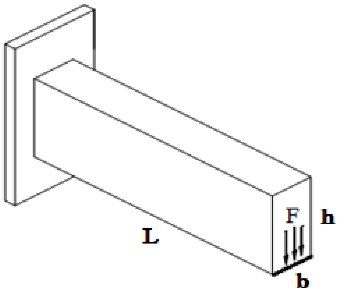
5.4. Example 4—Simply Supported Beam–Performance Characteristic Curve

In this problem is considered a simply supported beam under the loading and boundary conditions, as shown in Figure 10, with L = 40, h = 20 and F = 1 kN. The design domain is discretized into 40 × 20 × 40. The volume constraint is limited to 20% of the design domain during the whole evolutionary process. The material properties are Young’s modulus E = 100 GPa and Poisson’s ratio ν = 0.3, and the filtering radius is 1.5 mm. Figure 11 shows the optimal topologies in the solution domain for the models implemented. It is observed that the topologies of Figure 12a,b, respectively, ESO and SESO, whose design variables are the domain elements, have similar settings. Figure 12c,d, SERA and SIMP have the element density as design variables and presented different topologies. It is noteworthy again that SIMP converged with greater compliance, approximately 45% higher than other methods. The SESO, SERA, and ESO methods allow the withdrawal of elements with low compliance to improve the performance of the structure. Therefore, a characteristic performance curve for this continuum structure is shown in Figure 13. The weight of a structure is gradually reduced during the optimization procedure while compliance increases. The characteristic curve of the performance of a structure during the optimization procedure can be expressed through the weight of the structure and its strain energy, according to [25]. Structure performance informs the success of the stiffness-optimized design. In addition, it informs the designer of its viability.
The designer, when analyzing the curves below, should note that the optimal structure reached with compliance 5% greater than the initial compliance, in the graph C i / C 0 = 1.05 , is obtained with an approximate ratio volume V i / V 0 = 0.3 . Therefore, a volume less than 30%, for example: V i / V 0 = 0.26 is below the curve and, therefore, violates the compliance constraint, C i / C 0 = 1.1   because of the needed 10% greater compliance than the initial. Additionally, this structural design would not be feasible because it lacks the material to finish it. On the other hand, projecting the compliance ratio, C i / C 0 = 1.05 , to a point above the curve, V i / V 0 = 0.5 , the amount of volume is more than sufficient for executing the project; that is, the project is feasible, but it is oversized.
Therefore, the structural optimization methods SESO, SERA, and ESO can improve the performance of oversized structures while saving material. According to Figure 13, these structures meet the design conditions, are not oversized, and have resulted in considerable material savings, as indicated in [25]. In SIMP, this process is continuous, and the topology evolves by changing the modulus of elasticity continuously. Therefore, the SIMP characteristic curve graph is a parallel line to the compliance axis because the volume has a minimum variation in the order of 10 4 .
Figure 14 shows the surface graphs of these structures showing the differences between the optimal settings. The SERA and SIMP methods, based on density, presented very different topologies from the other two SESO and ESO methods. It is also observed that the SERA and ESO topologies are similar and have the same value for the objective function, which can characterize an optimal stationary, identical to these two methods. Moreover, it is worth noting that SESO, ESO, and SERA had similar computational costs; however, this was 5% higher than the SIMP method.

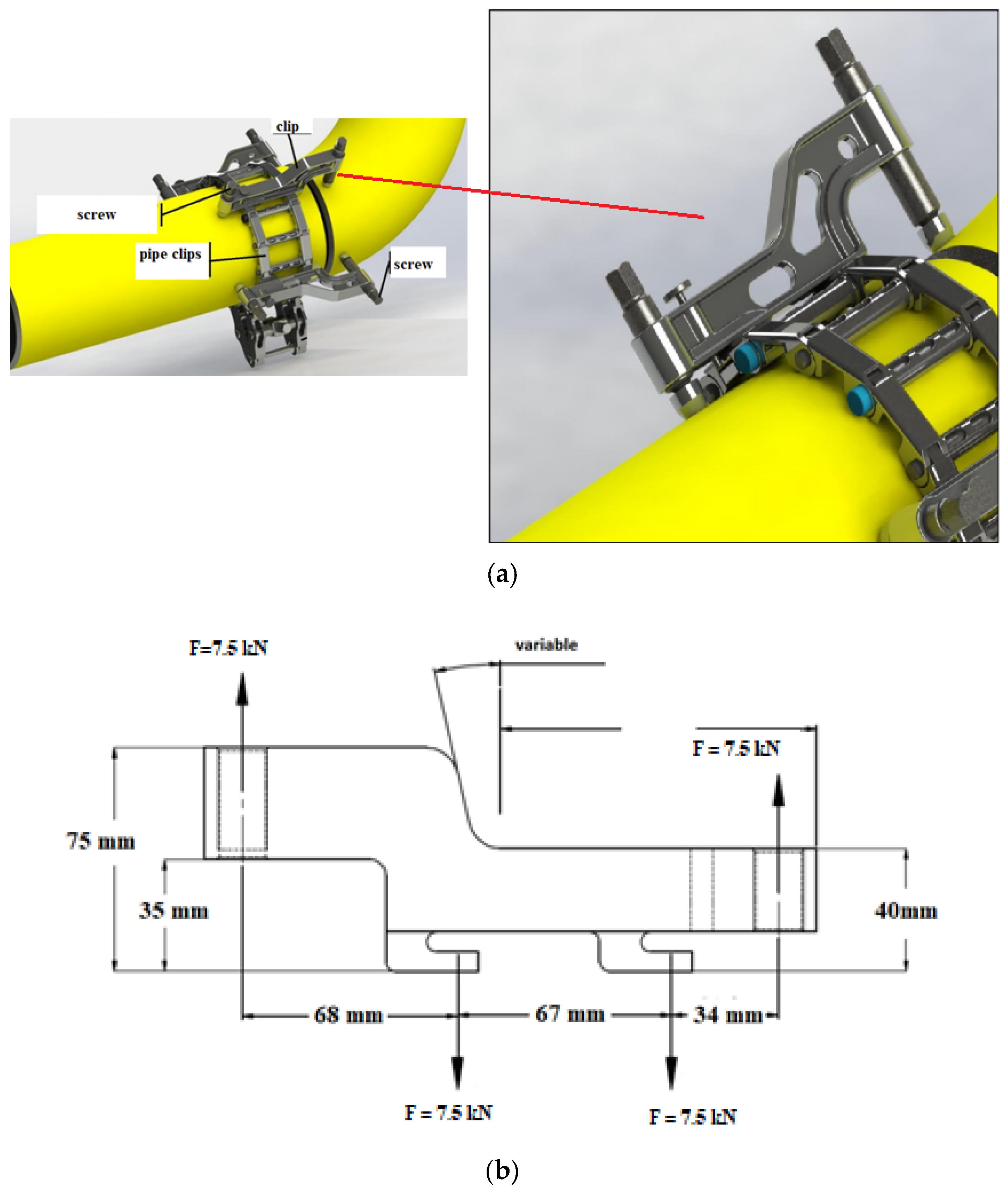
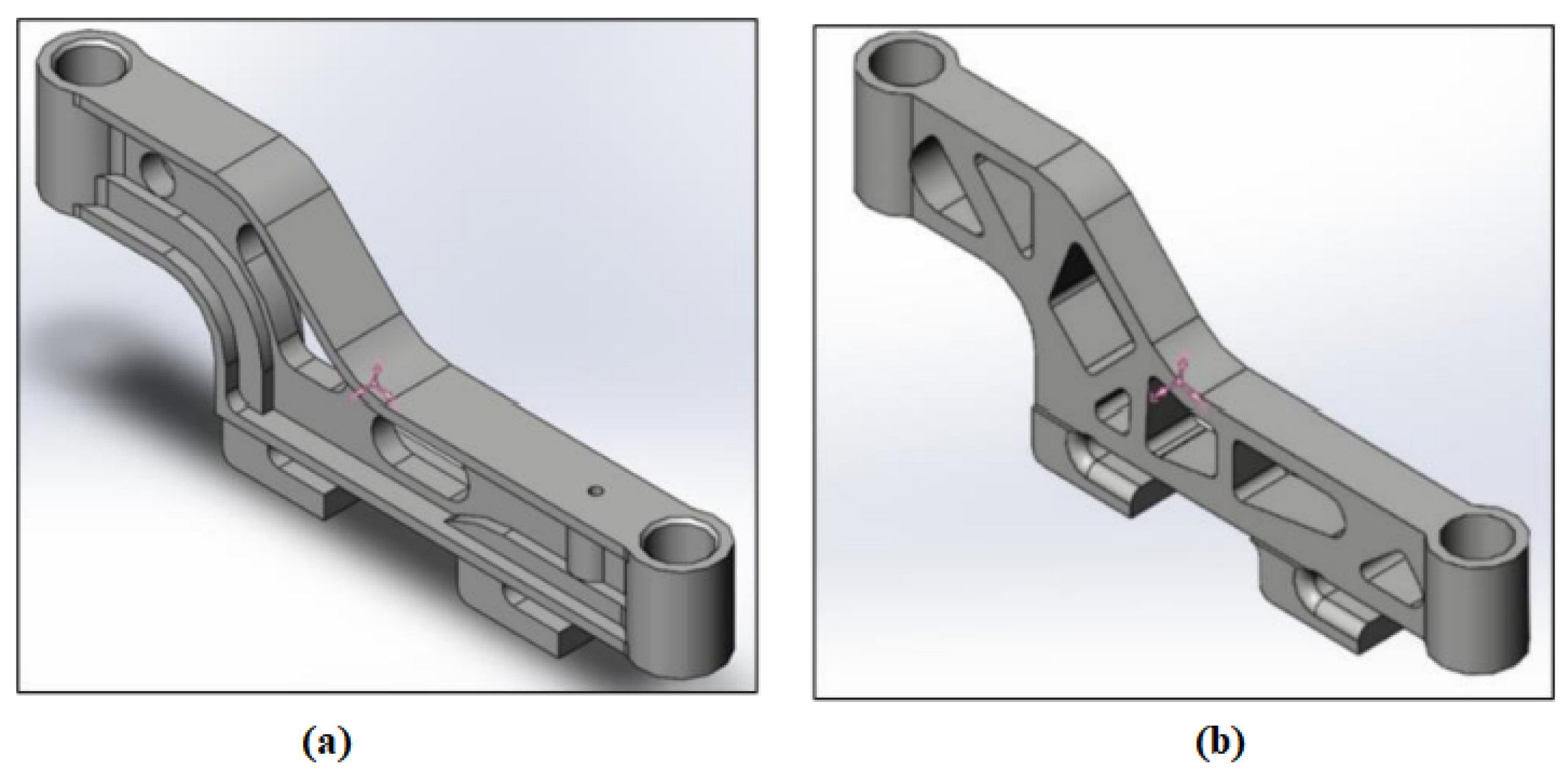
5.5. Example 5—Industrial Application: Flexible Coupler

The TO concepts for the manufacture and assembly of a welded industrial pipe are applied to evaluate the best topological configuration of a metal clamp, which is part of the member pipe tool called a flexible coupler. The Brazilian company called YPY Engineering [26] manufactures the model, where in Figure 15a can be seen the flexible coupler in the assembly of a tube-curve type, which has been obtained via an “empirical” process through CAE (Computer Aided Engineering) analysis and Figure 15b illustrates the design domain and boundary conditions for the flexible coupler composed of clips specially developed to form an adjustable strap according to the size of the pipe. TO is performed with the SESO method, which applies a Finite Element Analysis to a 180 × 75 × 8 geometry containing 57,120 hexahedral finite elements. The material properties are Young’s modulus E = 2.1 E 5   MPa and Poisson’s ratio ν = 0.3, the filtering radius is 1.5 mm, and the optimization parameters are R R = E R = 0.01 . The loads have a magnitude of 7.5   kN and are applied at four different points, as shown in Figure 15. The optimal topology is shown in Figure 16 with front and cross-sectional views, which was achieved with a final volume fraction of 0.25 and compliance of 7.333 kN·mm. After obtaining the optimal structure, tests of deflection and straining of the component were done using SolidWorks. The model optimized via SESO and post-processed in SolidWorks achieved a volume reduction of approximately 62% of the one proposed by [26], and Figure 17 shows that the model created through the TO procedure had seven cavities, compared to the three cavities of [26].

6. Conclusions

This article approaches four different TO methods based on compliance minimization procedures applied to 3D elastostatic problems. The SESO, SERA and ESO methods were implemented in Matlab code, and the results obtained are compared with the deterministic SIMP method. A free code, presented in [6], was used to introduce the methods mentioned above, in which a hexahedral finite element is used to discretize the design domain, and an elastic analysis is used to calculate the objective function in each method.
It is possible to conclude that the implemented models can generate optimal topologies that can support the loads applied under defined boundary conditions. Additionally, with the results presented, it is clear that the SESO and ESO methods, whose design variables are the domain elements, have very close optimal settings with a low computational cost. It is highlighted that these methods’ compliance is much lower than those presented with the SIMP method. It was observed that the four methods presented chessboard settings when the filter was disabled, implying an increase in compliance. Nevertheless, SERA and SIMP showed denser chessboard regions. It was also verified that the increase in the number of mesh elements provides an increase in the computational cost since the number of variables increases with the cube of the proportionality ratio of the mesh. In addition, the result presented for the synthesis of flexible mechanisms with the approaches proposed in this article showed good accuracy with the examples in the literature. Moreover, these models can be extended to incorporate constraints of stress, displacements, and natural frequency.

Author Contributions

The authors have been working together for over 9 years, and the tasks in this article were developed as follows: (1) H.L.S.—Implemented SERA-3D and SESO-3D programs in Matlab code. Responsible for writing and structuring the article. (2) V.S.A.—Implemented SERA and SESO codes. Responsible for reviewing the article. Participated in the data analysis of the numerical examples in the article. (3) F.d.A.d.N.—Contributions to the preparation of the article: reading, review and suggestions for examples. (4) V.D.D.A.—Implemented ESO-3D and participated in the data analysis of the numerical examples in the article. (5) M.D.S.C.—Suggested and wrote the discussion section and participated in the review of the article. All authors have read and agreed to the published version of the manuscript.

Funding

CNPq (National Council of Scientific and Technological Development) under Grant Number 30503/2018-5. FAPEMIG (Foundation for Research Support of Minas Gerais State) under Grant number TEC-PPM-00692-18 and Sao Paulo State Research Foundation (FAPESP) under Grant Number 2016/02327-5. Instituto Federal de Educação Ciência e Tecnologia de Minas Gerais (IFMG) under Grant Number.

Institutional Review Board Statement

Not applicable.

Informed Consent Statement

Not applicable.

Data Availability Statement

Not applicable.

Acknowledgments

The authors are grateful to the Instituto Federal de Educação Ciência e Tecnologia de Minas Gerais–IFMG, CNPq (National Council of Scientific and Technological Development) under Grant Number 30503/2018-5 and Number 315632/2020-8, CAPES (the Coordination for Improvement of Higher-Education Personnel), FAPEMIG (Foundation for Research Support of Minas Gerais State)and Grand number TEC-PPM-00692-18 and Sao Paulo State Research Foundation (FAPESP) under Grant Number 2016/02327-5 for their financial support.

Conflicts of Interest

The authors declare no conflict of interest.

References

  1. Sigmund, O. A 99 line topology optimization code written in Matlab. Struct. Multidiscip. Optim. 2001, 21, 120–127. [Google Scholar] [CrossRef]
  2. Andreassen, E.; Clausen, A.; Schevenels, M.; Lazarov, B.S.; Sigmund, O. Efficient topology optimization in MATLAB using 88 lines of code. Struct. Multidiscip. Optim. 2011, 43, 1–16. [Google Scholar] [CrossRef]
  3. Challis, V.J. A discrete level-set topology optimization code written in Matlab. Struct. Multidiscip. Optim. 2010, 41, 453–464. [Google Scholar] [CrossRef]
  4. Huang, X.; Xie, Y.M. Bi-directional evolutionary topology optimization of continuum structures with one or multiple materials. Comput. Mech. 2009, 43, 393–401. [Google Scholar] [CrossRef]
  5. Ansola Loyola, R.; Querin, O.M.; Garaigordobil Jiménez, A.; Alonso Gordoa, C. A sequential element rejection and admission (SERA) topology optimization code written in Matlab. Struct. Multidiscip. Optim. 2018, 58, 1297–1310. [Google Scholar] [CrossRef]
  6. Gebremedhen, H.S.; Woldemicahel, D.E.; Hashim, F.M. Three-dimensional stress-based topology optmization using SIMP mehod. Int. J. Simul. Multidiscip. Des. Optim. 2019, 10, A1. [Google Scholar] [CrossRef]
  7. Liu, K.; Tovar, A. An efficient 3D topology optimization code written in Matlab. Struct. Multidiscip. Optim. 2014, 50, 1175–1196. [Google Scholar] [CrossRef]
  8. Zegard, T.; Paulino, G.H. GRAND3—Ground structure based topology optimization for arbitrary 3D domains using MATLAB. Struct. Multidiscip. Optim. 2015, 52, 1161–1184. [Google Scholar] [CrossRef]
  9. Zegard, T.; Paulino, G.H. Bridging topology optimization and additive manufacturing. Struct. Multidiscip. Optim. 2016, 53, 175–192. [Google Scholar] [CrossRef]
  10. Borrvall, T.; Petersson, J. Large-scale topology optimization in 3D using parallel computing. Comput. Methods Appl. Mech. Eng. 2001, 190, 6201–6229. [Google Scholar] [CrossRef]
  11. Zuo, Z.H.; Xie, Y.M. A simple and compact Python code for complex 3D topology optimization. Adv. Eng. Softw. 2015, 85, 1–11. [Google Scholar] [CrossRef]
  12. Langelaar, M. Topology optimization of 3D self-supporting structures for additive manufacturing. Addit. Manuf. 2016, 12, 60–70. [Google Scholar] [CrossRef]
  13. Chi, H.; Zhang, Y.; Tang, T.L.E.; Mirabella, L.; Dalloro, L.; Song, L.; Paulino, G.H. Universal machine learning for topology optimization. Comput. Methods Appl. Mech. Eng. 2021, 375, 112739. [Google Scholar] [CrossRef]
  14. Brown, N.K.; Garland, A.P.; Fadel, G.M.; Li, G. Deep reinforcement learning for engineering design through topology optimization of elementally discretized design domains. Mater. Des. 2022, 218, 110672. [Google Scholar] [CrossRef]
  15. Kollmann, H.T.; Abueidda, D.W.; Koric, S.; Guleryuz, E.; Sobh, N.A. Deep learning for topology optimization of 2D metamaterials. Mater. Des. 2020, 196, 109098. [Google Scholar] [CrossRef]
  16. Simonetti, H.L.; Almeida, V.S.; Neto, L.O. A smooth evolutionary structural optimization procedure applied to plane stress problem. Eng. Struct. 2014, 75, 248–258. [Google Scholar] [CrossRef]
  17. Xie, Y.M.; Steven, G.P. A simple evolutionary procedure for structural optimization. Comput. Struct. 1993, 49, 885–896. [Google Scholar] [CrossRef]
  18. Ghabraie, K. The ESO method revisited. Struct. Multidiscip. Optim. 2015, 51, 1211–1222. [Google Scholar] [CrossRef]
  19. Ansola, R.; Veguería, E.; Alonso, C.; Querin, O.M. Topology optimization of 3D compliant actuators by a sequential element rejection and admission method. In IOP Conference Series: Materials Science and Engineering; IOP Publishing: Bristol, UK, 2016; Volume 108, p. 012035. [Google Scholar] [CrossRef]
  20. Yang, X.Y.; Xie, Y.M.; Steven, G.P. Evolutionary methods for topology optimisation of continuous structures with design dependent loads. Comput. Struct. 2005, 83, 956–963. [Google Scholar] [CrossRef]
  21. Sigmund, O.; Petersson, J. Numerical instabilities in topology optimization: A survey on procedures dealing with checkerboards, mesh-dependencies and local minima. Struct. Optim. 1998, 16, 68–75. [Google Scholar] [CrossRef]
  22. Bruns, T.E.; Tortorelli, D.A. Topology optimization of non-linear elastic structures and compliant mechanisms. Comput. Methods Appl. Mech. Eng. 2001, 190, 3443–3459. [Google Scholar] [CrossRef]
  23. Wang, M.Y. Mechanical and geometric advantages in compliant mechanism optimization. Front. Mech. Eng. China 2009, 4, 229–241. [Google Scholar] [CrossRef]
  24. Lau, G.; Du, H.; Lim, M. Convex analysis for topology optimization of compliant mechanisms. Struct. Multidiscip. Optim. 2001, 22, 284–294. [Google Scholar] [CrossRef]
  25. Simonetti, H.L.; Almeida, V.S.; de Assis das Neves, F.; Del Duca Almeida, V.; de Oliveira Neto, L. Reliability-Based Topology Optimization: An Extension of the SESO and SERA Methods for Three-Dimensional Structures. Appl. Sci. 2022, 12, 4220. [Google Scholar] [CrossRef]
  26. Ypycom. Ferramentas Especiais. “Fixação com Precisão”. Available online: https://ypycom.com.br (accessed on 13 February 2023). (In Portuguese).
Figure 1. Spatial filter, elements i, j and distance d.
Applsci 13 06215 g001
Figure 2. Long Cantilever beam subjected to tip point load.
Applsci 13 06215 g002
Figure 3. Design domain with essential and natural boundary conditions (measures in mm).
Applsci 13 06215 g003
Figure 4. Optimal topology—(a) SESO, (b) ESO, (c) SERA and (d) SIMP.
Applsci 13 06215 g004
Figure 5. Optimal topology—(a) SESO, (b) ESO, (c) SERA and (d) SIMP.
Applsci 13 06215 g005
Figure 6. Design domain of a channel beam Adapted from [20], measures in meters.
Applsci 13 06215 g006
Figure 7. Optimal topology—(a) SESO, (b) SERA, (c) ESO and (d) SIMP.
Applsci 13 06215 g007
Figure 8. Compliance by Iteration—(a) SESO, (b) ESO, (c) SERA and (d) SIMP.
Applsci 13 06215 g008
Figure 9. Design domain and boundary conditions of the inverter mechanism.
Applsci 13 06215 g009
Figure 10. (a) SESO, (b) SERA, (c) ESO, and (d) SIMP.
Applsci 13 06215 g010
Figure 11. Design domain, boundary, and loading conditions.
Applsci 13 06215 g011
Figure 12. Optimal topology—(a) ESO, (b) SESO, (c) SERA and (d) SIMP.
Applsci 13 06215 g012
Figure 13. Performance characteristic curve for structures with compliance constraints: (a) SESO, (b) ESO, (c) SERA, and (d) SIMP.
Applsci 13 06215 g013
Figure 14. Surface graphs for optimal topology: (a) SERA, (b) SESO, (c) SIMP, and (d) ESO.
Applsci 13 06215 g014
Figure 15. (a) metal clamp model, [26]; (b) Design domain and boundary conditions.
Applsci 13 06215 g015
Figure 16. Topology optimal: (a) frontal view—SESO and (b) cross view—SESO.
Applsci 13 06215 g016
Figure 17. Topology optimal—(a) YPY ENG 2018 and (b) SESO.
Applsci 13 06215 g017
Table 1. Comparing Topology Optimization algorithms with a mesh-independency filter.
MethodsParametersNumber of
Iterations/Costs
Optimal Settings/Compliance
ESO R R = 0.02
E R = 0.02
r m i n = 1.5
i t e r = 200
t i m e = 815.65   s
Applsci 13 06215 i001
C = 1593.4232
SERA P R = 0.02
S R = 1.02
B = 0.007
r m i n = 1.5
i t e r = 200
t i m e = 775.51   s
Applsci 13 06215 i002
C = 1599.4558
SESO R R = 0.02
E R = 0.02
r m i n = 1.5
i t e r = 200
t i m e = 887.90   s
Applsci 13 06215 i003
C = 1593.4232
SIMP p = 3
M O V E = 0.02
r m i n = 1.5
i t e r = 200
t i m e = 853.08   s
Applsci 13 06215 i004
C = 2255.9835
Table 2. Comparing Topology Optimization algorithms without a mesh-independency filter.
MethodsParametersNumber of
Iterations/Costs
Optimal Settings/Compliance
ESO R R = 0.02
E R = 0.02
r m i n = 1.5
i t e r = 135
t i m e = 718.01   s
Applsci 13 06215 i005
C = 1688.1480
SERA P R = 0.02
S R = 1.02
B = 0.007
r m i n = 1.5
i t e r = 131
t i m e = 647.09   s
Applsci 13 06215 i006
C = 1658.9346
SESO R R = 0.02
E R = 0.02
r m i n = 1.5
i t e r = 135
t i m e = 689.15   s
Applsci 13 06215 i007
C = 1688.1480
SIMP p = 3
M O V E = 0.02
r m i n = 1.5
i t e r = 57
t i m e = 292.92   s
Applsci 13 06215 i008
C = 1968.4670
Table 3. Results obtained for the L-shaped structure.
MethodParametersNumber
of Iterations
Objective FunctionComputational Cost (Minutes)
SESO R R = E R = 0.02 10065.7449.72
ESO R R = E R = 0.02 10065.8849.57
SERA S R = 1.15 ,
B = 0.007
P R = 0.02
10064.8348.39
SIMP p = 3
  M O V E = 0.02
10092.0458.70
Table 4. Comparing Topology Optimization algorithms for compliant mechanism (Mechanical Advantage).
MethodSESOSERAESOSIMP
GAApplsci 13 06215 i009Applsci 13 06215 i010Applsci 13 06215 i011Applsci 13 06215 i012
Time
(s)
19.4219.8019.8425.04
Iteration60616160
Contour graphicsApplsci 13 06215 i013Applsci 13 06215 i014Applsci 13 06215 i015Applsci 13 06215 i016
Objective FunctionApplsci 13 06215 i017Applsci 13 06215 i018Applsci 13 06215 i019Applsci 13 06215 i020
Surface graphicsApplsci 13 06215 i021Applsci 13 06215 i022Applsci 13 06215 i023Applsci 13 06215 i024
Table 5. Comparing Topology Optimization Algorithms for Compliant mechanism (Geometrical Advantage).
MethodSESOSERAESOSIMP
GAApplsci 13 06215 i025Applsci 13 06215 i026Applsci 13 06215 i027Applsci 13 06215 i028
Time (s)19.7419.9920.1021.38
Iteration60616160
Contour graphicsApplsci 13 06215 i029Applsci 13 06215 i030Applsci 13 06215 i031Applsci 13 06215 i032
Objective FunctionApplsci 13 06215 i033Applsci 13 06215 i034Applsci 13 06215 i035Applsci 13 06215 i036
Surface graphicsApplsci 13 06215 i037Applsci 13 06215 i038Applsci 13 06215 i039Applsci 13 06215 i040
Disclaimer/Publisher’s Note: The statements, opinions and data contained in all publications are solely those of the individual author(s) and contributor(s) and not of MDPI and/or the editor(s). MDPI and/or the editor(s) disclaim responsibility for any injury to people or property resulting from any ideas, methods, instructions or products referred to in the content.

