Calibration and Validation of a Measurements-Independent Model for Road Traffic Noise Assessment

Featured Application

The road traffic noise predictive model presented in this paper can be calibrated without field measurements and can be applied in several traffic conditions, with an average error lower than 2 dBA.

Abstract

The assessment of road traffic noise is very important for the health of people living in urban areas. Noise is usually assessed by field measurements, and predictive models play an important role when experimental data are not available. Nevertheless, when they are based on regression techniques, predictive models suffer from the drawback of strong dependence on the calibration data. In this paper, the authors present a regressive model calibrated on computed noise levels without the need for field measurements. The independence from field measurements makes the model flexible and adjustable for any road traffic condition possible. A multilinear regression technique is applied to establish the correlation between the computed equivalent noise levels and several independent variables, including, among others, traffic flow and distance. The model is then validated on a large field measurement database to check its efficiency in terms of prediction accuracy. The validation is performed both via error distribution analysis and using different error metrics. The results are encouraging, showing that the model provides good results in terms of the average error (less than 2 dBA) and is not susceptible to the presence of outliers in the input data that correspond to unconventional conditions of the traffic flow.

1. Introduction

Noise, especially when coming from road traffic, is one of the most pervasive pollutants. Especially in urban areas, a large percentage of the population is estimated to be exposed to noise levels largely exceeding the limits fixed by laws [1]. Since urbanization has expanded, people are constantly in contact with a large number of vehicles, and continuous exposure to the generated noise levels leads to physical and psychological detriments, such as high blood pressure and sleep deprivation, together with mental disorders [2,3,4]. Much evidence for this correlation can be found in the literature; for example, some works show that intrusive sounds can severely affect sleep [5] and mental health [6]. Traffic noise in urban areas is not only related to the direct exposure of pedestrians but also accounts for people in their houses since many buildings can be reached by high noise levels [4]. For this reason, the estimation of the amount of noise in urban areas is very important for human health assessments [7].

Aside from the measurement of such noise levels to ease inhabitants’ conditions, many different models for the estimation of noise in a certain area can be found, all with the common goal of best describing the noise level, starting with different parameters such as the number and type of passing vehicles, the distance of the receiver from the noise source (the vehicle itself), the presence of roundabouts and/or intersections [8], and speed, as well as also climate conditions [9], the location or absence of acoustic barriers, and so on [10,11]. Such a comprehensive traffic noise model could provide a proper prediction of noise levels to assist authorities and planners in setting up and applying noise mitigation measures, for example, for the design of new roads or for the renewal of existing ones [7]. Models can be generated at many different levels of complexity and efficiency, and a proper balance between these two aspects is necessary to implement a practical and effective one. For instance, computational fluid-dynamic approaches are often used in the automotive and airplane industries to design noise reduction systems [12].

Generally speaking, the main types of models are statistic, analytic, microscopic, macroscopic, semi-dynamic, and dynamic [13]. Focusing on time dependence, the models are usually built to predict noise indices over a certain period of time dependent on selected independent variables [14]. Variables chosen can vary in type and number, but the most used are certainly traffic volume, the percentage of heavy vehicles, and the distance between the source and receiver. Additional parameters considered can be the road slope, the texture of the asphalt, the average speed of the flow, and the weather conditions. These kinds of models are flexible and easy to use, including for non-expert users. They are basically functions in which selected “independent” parameters are related to the noise level through proper coefficients. Their efficiency strongly depends on the calibration step, that is, the process that establishes and details the correlation between each parameter and the noise level. When this process is run through regression using in-field-measured data, the model belongs to the statistical category.

The importance of this process is evident when trying to apply such a model to a road traffic framework very different from the one used for calibration. In such cases, in fact, the efficiency of the model output can easily be lowered. For this reason, many national laws establish which model can be used in the country. Some of the models adopted in national regulations are listed in Ref. [15]: the CoRTN model in the United Kingdom [16], the RLS90 model in Germany [17], the NMPB model in France [18], the ASJ model in Japan [19], and the SONROAD model in Switzerland [20]. In such a complex scenario, the European Union issued the European Noise Directive related to the assessment and management of environmental noise, in which the main definitions and rules are provided to member states [21]. In particular, the noise indicators are defined as the equivalent continuous sound levels calculated for the day (L_d), evening (L_e), or night (L_n) timespans, as well as for the entire day (L_den). The latter indicator includes a penalty for evening and night hours. The effort to harmonize noise assessment for many sources, including road traffic, has led to the development of the CNOSSOS model, which is nowadays the reference model in Europe [22]. Regardless of the considered model, all of them assess the noise levels using various indicators, usually estimated at a fixed distance over a given time range. The most important is the equivalent continuous sound level, L_eq, which is the constant sound level in dBA, with the same total sound energy as the fluctuating level measured in the considered timespan (such as 15 min, 1 h, a day, an evening, a night).

In the present paper, developing an idea proposed by Afandizadeh et al. in Ref. [23], the authors used a multilinear regressive model for the evaluation of noise from traffic in which the estimation of the noise level is implemented from computed data and not from real ones. The proposed model, in fact, aims to predict noise equivalent levels produced by road traffic, calibrating on a dataset of computed noise levels. The independent variables used for the calibration are the total traffic volume, the percentage of medium and heavy vehicles, the mean speed of each type of vehicle, and the distance between the center of the highway and the receiver. The computed level database is obtained with a random sampling of the independent variables listed above that feed the formula proposed by Quartieri et al. [14]. Once the computed level database is obtained, a multiple linear regression technique—implemented with a self-written Python routine—is used to establish the correlation between the independent variables and the L_eq,t on a fixed time range, t. This approach overcomes some shortcomings of the classic and statistical models. Firstly, the model can be calibrated without any field measurements by using a computed set of data. It is known, in fact, that model efficiency usually decreases when applying models to a site different from the ones where they were calibrated [16]. Secondly, the model can be recalibrated quickly when needed to include different traffic road conditions. Another advantage of this approach is that its independence from measured data makes it suitable to be applied to estimate the impact of traffic noise even for roads that do not yet exist, providing useful information when designing new roads in urban or non-urban areas.

The outputs of the model are then validated with measured data coming from a Long-Term Monitoring Station (LTMS) system installed in the city of Saint-Berthevin (France) by the Université Gustave Eiffel and Unité Mixte de Recherche en Acoustique Environnementale (UMRAE), Nantes. This study aims to deepen the understanding of physical phenomena in the field of environmental acoustics, correlating noise measurements at different acoustic masts with meteorological parameters collected over a period of ten years. The model was applied to part of the dataset and a prevision of the hourly equivalent level—L_eq,h—was performed. The simulated data were compared with the measured ones to evaluate the goodness of the model. The same process was repeated in a 15 min timespan to check the robustness of the model in a different time range and on a larger set of data. The results show, in both cases, how the model is able to provide a good approximation of noise level distributions. The performance of the model has been quantitatively estimated via error distribution analysis and error metrics.

2. Materials and Methods

An algorithm for the generation of a 2000-occurrences data frame was implemented. Each row of the data frame represents a fictive traffic flow situation in which different vehicles are moving at a given average speed, and the impact of the noise can be evaluated in variable timespans—hours, fractions of an hour, or multiples of an hour—at variable distances. Vehicles flowing can belong to “light”, “medium”, or “heavy” vehicle categories. According to French regulations [24], for instance, “light” vehicles are common passenger cars with a gross weight of less than 4500 kg, “medium” vehicles have a gross weight below 3500 kg but a length equal to or larger than 3 m, and “heavy” vehicles exceed 3500 kg of gross weight.

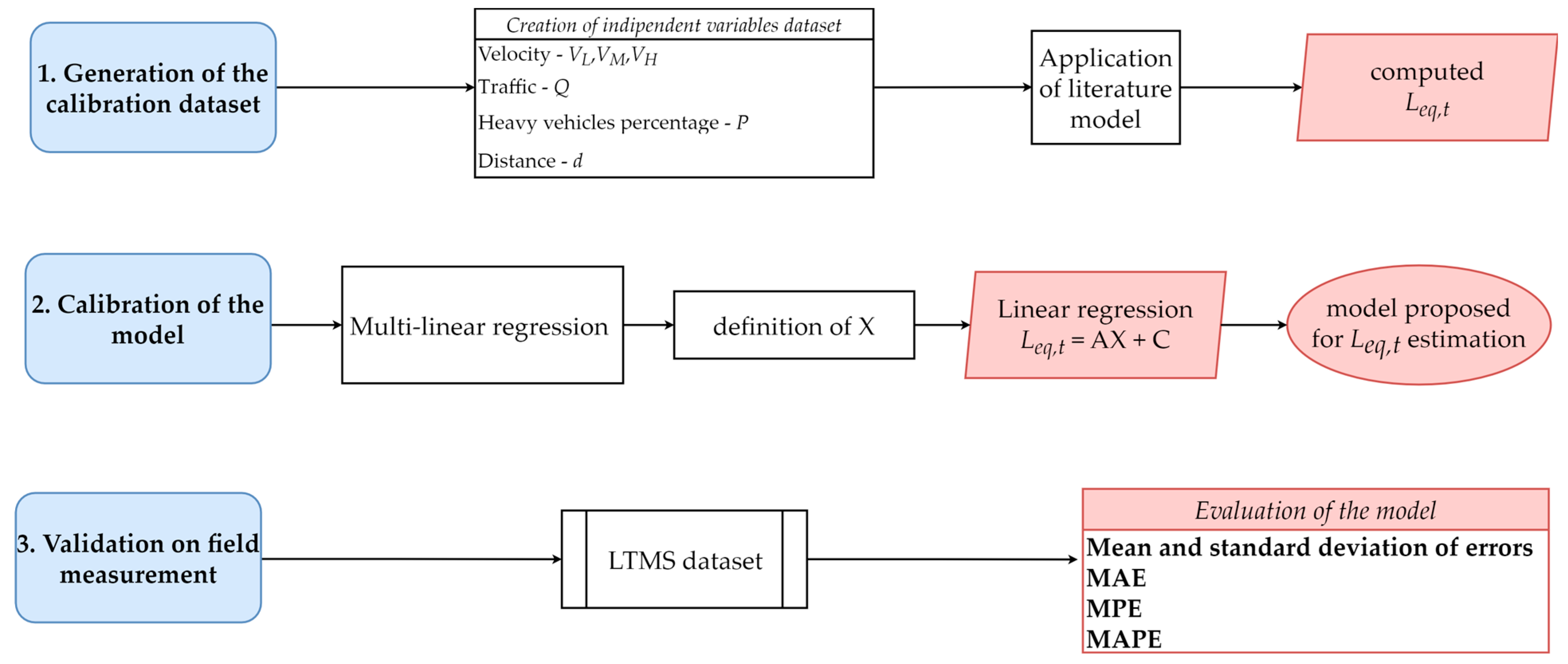
The first step was the generation of a computed dataset, and it consists of the random generation of 2000 fictitious traffic conditions identified by 6 independent variables and the subsequent calculation of noise equivalent levels. The chosen six independent variables are as follows: volume of traffic (Q), expressed as the number of moving vehicles per hour; average velocity of each vehicle type (light vehicles, medium vehicles, and heavy vehicles, respectively, V_L, V_M, and V_H); percentage, P, of heavy vehicles over the total flow; and the distance between the center of the highway and the base of the acoustic masts (receiver), d.

The choice of working with average speeds and with a single value for the traffic flow for both directions was necessary to reduce the complexity of the model and optimize the computational effort. However, this choice may represent a limitation to the model, since some hours of the day, in particular circumstances, are characterized by a large variation in single vehicle speed and by a strong asymmetry in the flow’s directions.

The range of the values of the independent variables are as follows: P values range from a minimum of 0 to a maximum of 20%, with steps of 0.1%; V_L values range from 30 to a maximum of 130 km/h, with steps of 5 km/h; V_M values span from 30 to a maximum of 100 km/h, with steps of 5 km/h; and V_H values span from 30 to a maximum of 80 km/h, with steps of 5 km/h. Variable d values range from 10 to 100 m, with steps of 1 m. The independent variables were chosen with two different criteria: a ladder function and a random function. The execution of the functions is sequential, as indicated by the pseudocode available in the Supplementary Materials, where the ranges of each variable value are also reported in detail.

The first independent parameter chosen is Q, and it is built with the ladder approach, which is a simple function generating integer values from a minimum of 10 to a maximum of 2000 veh/h, with intervals of 10 veh/h. For each of these flow generation step, the other variables are added, finalizing the construction of the dataset. Specifically, for every Q value sampling step, the algorithm implements 20× loops to associate all the other independent variables, which were chosen using the second criterion, i.e., randomly. For each Q, then, 20 casual combinations of the other independent values (P, V_L, V_M, V_H, d) are generated, completing each final occurrence, now described by the whole set of independent variables and useful for the L_eq,h calculation. The random choice of the values of the independent variables is performed in a specific order: after Q, P values are generated by randomly picking a value from the described interval. Once a P value is obtained, the number of medium and heavy vehicles is calculated from P by rounding the results to obtain an integer number and dividing it by two (so that the number of heavy and medium vehicles is the same for each occurrence). Finally, the number of light vehicles is obtained by subtracting medium and heavy vehicles by the whole of Q. After that, values of distance, d, are casually chosen from the indicated range, and then, the same approach is used for velocities, which are randomly chosen in this order: V_L, V_M, and V_H. In this last case, the generation of velocities is completely random, but some constrictions are fixed. Specifically, the velocities of the medium and heavy vehicles are forced to be lower than the velocity of light vehicles. The actual range of the medium and heavy vehicles, then, has a fixed lower limit but a moving upper limit so that a case where heavy vehicles move faster than light ones never happens. Please note that, for each row of the dataset, the velocity value is applied to all the vehicles involved. The first phase of the creation of the dataset, then, ends with a set of randomly set conditions of road traffic flow. Please note each casual combination is generated with a given seed to assure reproducibility (see “Pseudocode” image in the Supplementary Materials, line 2).

Once the whole dataset is generated, the independent variables are used to compute the corresponding values of L_eq,h, completing the dataset. L_eq,h computing starts from the computing of the power levels, L_W,L, L_W,M, and L_W,H, which are obtained by using a Noise Emission Model (NEM) [25]. These NEMs usually provide the source power level as a function of either the speed of a single vehicle or the average velocity of the flow. In this paper, the REMEL model was used, as reported in the work of Wayson et al. [26]:

$$\left\{\begin{array}{c}{L}_{W,L}=31.13 {\log }_{10}\left(V_L\right)+12.77+20 {\mathrm{l}\mathrm{o}\mathrm{g}}_{10}\left(d_0\right)+11\\ L_{W,M}=18.765 {\log }_{10}\left(V_M\right)+43.697+20 {\mathrm{l}\mathrm{o}\mathrm{g}}_{10}\left(d_0\right)+11\\ L_{W,H}=12.831 {\log }_{10}\left(V_H\right)+58.27+20 {\mathrm{l}\mathrm{o}\mathrm{g}}_{10}\left(d_0\right)+11\end{array}\right.$$

(1)

The choice of the Noise Emission Model (NEM) is arbitrary, and the proposed formulation permits the potential application of different NEMs by only modifying the structure of Equation (1). In particular, this modular approach can fit any existing framework, including CNOSSOS-EU, which is suggested as a reference model by the EU. The choice of specific NEMs, which include the noise emission of hybrid/electric cars [27,28], could also address the necessity of properly simulating changes in the circulating fleets. The influence of different NEMs and various propulsion systems on the validation results could be further studied in a future paper.

Once the power level is obtained, the sound exposure levels (SEL) for each type of vehicle involved are obtained following the set of Equation (2), as reported in the work of Quartieri et al. [14].

$$\left\{\begin{array}{c}{SEL}_L=10 {\log }_{10}\left(Q_L\right)+L_{w,L}-20{\mathrm{l}\mathrm{o}\mathrm{g}}_{10}\left(d\right)-11\\ {SEL}_M=10 {\log }_{10}\left(Q_M\right)+L_{w,M}-20{\mathrm{l}\mathrm{o}\mathrm{g}}_{10}\left(d\right)-11\\ {SEL}_H=10 {\log }_{10}\left(Q_H\right)+L_{w,H}-20{\mathrm{l}\mathrm{o}\mathrm{g}}_{10}\left(d\right)-11\end{array}\right.$$

(2)

In these equations, the sound exposure levels (SEL) are computed as a function of the number of vehicles moving (Q_L, Q_M, and Q_H, respectively, the number of light, medium, and heavy vehicles); the power levels, L_W; and the distance from the receiver. The constant value, 11, is related to the assumption of the spherical propagation of the noise with an absorbing surface. Equations (1) and (2) are used to finally compute the L_eq,h values with Equation (3):

$$L_{eq,h}=10 \log \left(\frac{1}{3600}\right)+10 \log \left({10}^{\frac{{SEL}_L}{10}}+{10}^{\frac{{SEL}_M}{10}}+{10}^{\frac{{SEL}_H}{10}}\right)$$

(3)

In this formulation, the sound level is a function of the sound level emitted by each type of vehicle passing, and it is computed over the whole span of 3600 s, i.e., an hour. The idea is that the overall sound level is obtained by the (logarithmic) sum of the sound exposure levels produced by the three considered vehicle types, divided by one hour (3600 s). This constant can be adjusted for different timespans by simply modifying the denominator value in the subject of the first logarithm. Here ends the second phase of the first step of the generation of the algorithm.

The second step is the calibration of the model itself. The first phase of the calibration is the implementation of a multiple regression technique, by which the dependencies existing between the L_eq,h levels and all six independent variables can be found. Equation (4) shows the details of this multilinear regression.

$$L_{eq,h}=c_1{A}_1+c_2{A}_2+{c_{1}A}_3+{c_{1}A}_4+{c_{1}A}_5+{c_{1}A}_6+m_1$$

(4)

In Equation (4), A₁ is $\log Q$, A₂ is $\log V_L$, A₃ is $\log V_M$, A₄ is $\log V_H$_, A₅ is $\log P$_, and A₆ is $\log d$_. In the same equation, c₁, c₂, etc., are the coefficients of the multilinear regression and m₁, the intercept. The multiple linear regression accounts for the contemporary contributions of all variables, establishing the best-fitting model for the data supplied. In the second phase of the second step, the coefficients of the multiple linear regression are used as in Equations (5) and (6) to retrieve, from a univariate linear regression, the final calibration of the model. Specifically, in Equation (5), the linear dependence between the L_eq,h values and the same set of data, weighted by the coefficients retrieved in the previous multilinear regression, is assumed.

$$L_{eq,h}=cX+m_2$$

(5)

Namely, c is the coefficient of the regression, m₂ is the intercept, and X is the sum of the coefficients of the multiple linear regression multiplied by the data of the calibration model according to Equation (6):

$$X=\left(c_1\log Q\right)+\left(c_2\log V_L\right)+\left(c_3\log V_M\right)+\left(c_4\log V_H\right)+\left(c_5\log P\right)+\left(c_6\log d\right)$$

(6)

Multilinear regression, then, is a procedure used to compare the contemporary contributions of all the independent variables to the final L_eq,h values, and it provides a coefficient for each variable, together with an intercept. Please note that the coefficients do not simply represent the single dependence of the L_eq,h values from a variable; rather, they represent the influence of every single variable when the overall convergence is achieved. An analysis of the residuals is performed to assess the calibration process results.

The third and last step is the validation of the model with field measurements, which was performed using the long-term monitoring station (LTMS) database provided free for scientific purposes by the Université Gustave Eiffel, Nantes, France [29]. In this long-term database, data coming from several monitoring stations—acoustic, meteorological, road traffic, and ground impedance—located in the city of Saint-Berthevin (France) have been collected for 10 years and made available in a whole and unique database, at a base time of 15 min, referring to the period from 2002 to 2007 [29]. For the presented application, the authors considered the acoustic and traffic data and, specifically, the measurements of a reference sound level meter, which was positioned at 5 m height and at a fixed distance of 12.5 m from the center of the carriageway. The database was used to validate the goodness of the model by evaluating the error calculated as the difference between the measured equivalent levels and model simulations. Apart from the error distribution analysis, MAE (mean absolute error), MPE (mean percentage error), and MAPE (mean absolute percentage error) metrics were used for a quantitative evaluation of the model’s performance when applied to the dataset.

The three steps of the complete process described above are graphically summarized in the following flowchart (Figure 1).

3. Results and Discussions

In this section, the results of the procedure described above are presented and discussed thoroughly.

3.1. Simulation and Calibration Results

Data obtained from simulations of the traffic flow performed in the first step of the procedure described in Section 2 were collected in a unique dataset with a length of 2000 rows, representing light and heavy vehicles at different speeds at the center of the carriageway. This dataset simulates the collection of the independent values used for the computing of L_eq,h according to Quartieri et al. [14]. In each step of Q values, 10 different combinations of velocities, the percentage of heavy vehicles, and the distance are set, maximizing the combination of possible flow conditions simulated.

Table 1. Preview of the free flow traffic dataset showing some of the occurrences.

Q (veh/h)	VL (km/h)	VM (km/h)	VH (km/h)	P (%)	d (m)	Computed Leq,h (dBA)
10	80	70	75	13.1	66	37.2
10	70	30	55	14.7	84	32.8
10	55	30	35	15.7	34	38.0
10	65	30	45	3.3	89	28.2
10	100	50	65	5.4	10	53.0
…	…	…	…	…	…	…
100	50	30	30	5.4	62	39.5
100	100	85	45	7.6	54	49.0
100	50	30	40	11.4	12	55.7
100	60	40	60	6.4	43	45.6
100	55	55	35	13.3	69	41.9
…	…	…	…	…	…	…
1000	50	50	30	14.6	21	61.4
1000	95	45	50	7.3	18	67.6
1000	75	75	75	13.8	47	59.0
1000	90	80	55	10.2	66	56.5
1000	110	35	40	4.4	73	57.0
…	…	…	…	…	…	…
2000	80	75	60	14.4	16	71.4
2000	45	45	35	18.4	32	61.2
2000	70	70	50	5.8	89	53.7
2000	90	55	60	17.3	75	58.8
2000	60	40	55	13.7	89	53.8

shows a selection of lines from the used dataset. It is worth noting that the hourly L_eq,h value corresponding to very low values of vehicle flows are the levels produced just by the source vehicle, neglecting any other source that can be active in the area under study. This confirms that the model is computing the noise coming from road traffic only, and, thus, it could lead to underestimation when comparing it with field-measured data since it does not account for background noise. The introduction of a correction for background noise is under study and will be included in future papers to extend the range of the applicability of the model.

The creation of the dataset was guided by the idea of reflecting as wide a range of traffic as possible in order to create a final model able to efficiently perform at many different sites. For example, the volume of traffic, going from a minimum of 10 to a maximum of 2000 vehicles per hour, easily reflects traffic in both night and daily hours and even discriminates traffic in rush times (e.g., cars going to or coming back from work). As for velocities, a minimum speed of 30 km/h makes the model suitable to cover urban area conditions, while the peak speed reflects the cars moving at maximum velocity established by law for highways. The interconnection between the two variables, on the other hand, makes the model capable of distinguishing between standard situations (completely free flow, no obstacles, no congestion) and particular ones (intersections, presence of obstacles inducing sudden slowing down, congestion). It is also interesting to note the possibility offered by the model of evaluating the interconnection between the velocities of the different vehicle types since the inserted constraint makes the model more adherent to the real condition in which speed limits decrease with an increase in vehicle weight.

A closer look at the dataset makes evident that the strictest dependence is the one between L_eq,h and d since the highest values of emitted noise (L_eq,h in the fourth quartile of the distribution) are always related to the lowest values of d (first quartile of the distribution). This connection will be confirmed by the results of the multiple linear regression (see below).

The interdependence between the variables for the generation of the noise levels is clear when performing the multilinear regression technique, which was performed by using statsmodel, a Python library for statistical analysis. The library permits us to tune the regression calculation by adjusting several parameters in order to best fit the data and minimize errors. Three different models of linear regression have been tested: the Generalized Linear (GLS), the Ordinary Least Squares (OLS), and the Weighted Least Squares (WLS) models. The results were identical between the models in terms of coefficients, R², BIC, and AIC; then, the authors decided to apply the OLS model.

Table 2. Multilinear regression for the calibration of the model.

Model:	OLS
Df Model:	6
R-squared:	0.986
Log-Likelihood:	−2664.5
AIC:	5343
BIC:	5382
Intercept	27.362713
Coeff. log(Q)	10.022377
Coeff. log(VL)	19.902456
Coeff. log(VM)	1.382846
Coeff. log(VH)	1.921894
Coeff. log(P)	2.825697
Coeff. log(d)	−25.699334

shows the results of the linear regression between L_eq,h and the independent variables. Values of all the intercepts and regression coefficients are listed, together with R², AIC, and BIC.

The results of the multilinear regression indicate how distance, d, is the independent variable that most affects the L_eq,h values, contributing at the highest level to the variance in the model, followed by the velocities of light vehicles, V_L and Q. The distance dependence from L_eq,h is also the only one that is inverse with a negative coefficient, as expected (the higher the distance, the lower the L_eq,h value).

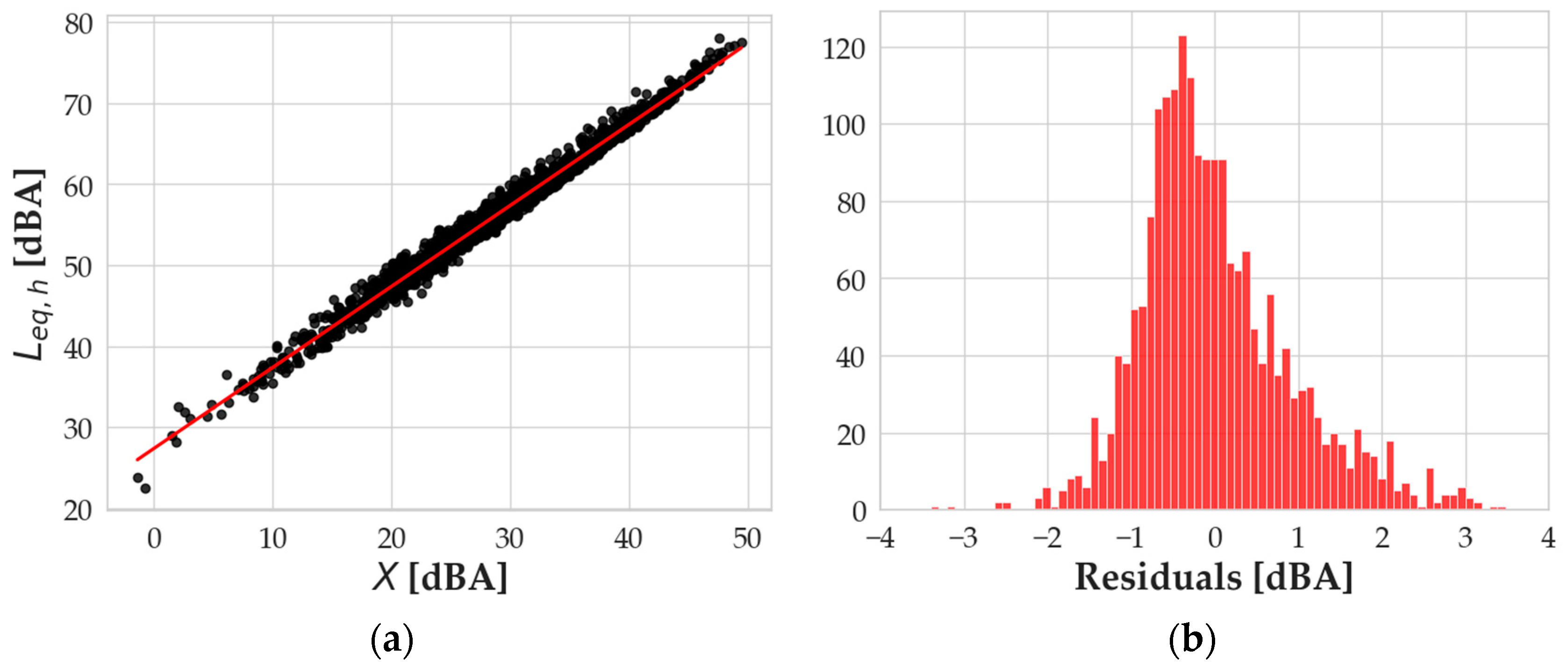
The calibration step goes on with a second linear regression, univariate, which was implemented by correlating L_eq,h as a function of all the independent values together, according to the X variable defined in Equation (6). The results of the regression are reported in Figure 2a. Figure 2b shows a distribution of the residuals that presents a mean value that is basically null (5.4 × 10⁻¹⁵ dBA) and a standard deviation of 0.92 dBA. The kurtosis index is 1.07, making the distribution slightly “leptokurtic”, and the skewness is 0.69, meaning that its right tail is slightly more pronounced than the left one. 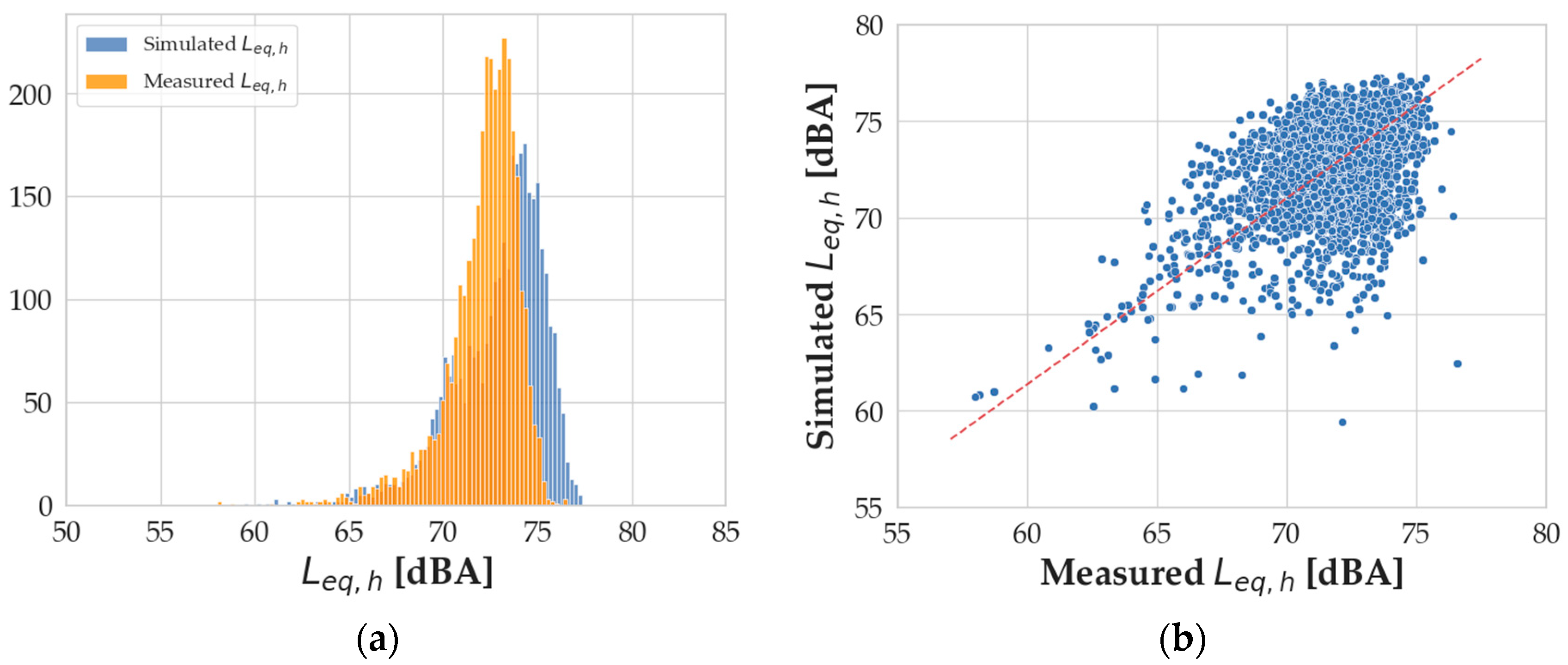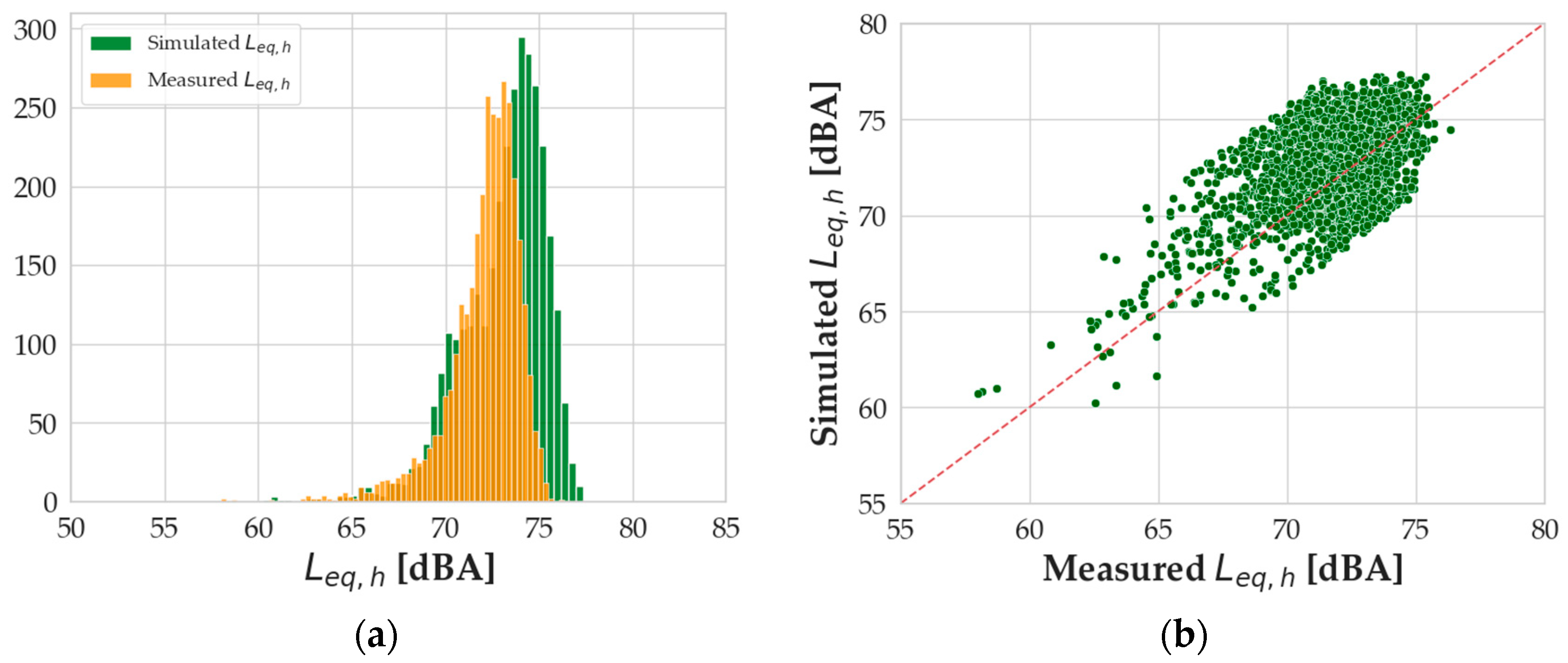Figure 3 shows the distributions of L_eq,h values simulated by the presented model and the L_eq,h measured and reported in the original database, as well as the scatterplot between the two sets of noise levels.

3.2. Validation of Field Measurements

Once the model was calibrated, its validity was tested by simulating the L_eq,h of road traffic flows observed in a real case study. The used dataset is the aforementioned dataset built by the Université Gustave Eiffel of Nantes in the city of Saint-Berthevin. The experimental setup was made of five acoustic masts positioned at different distances from the road and at two heights from the ground. Since the aim of this work was not focused on propagation issues, only measurements coming from the closest receiver to the carriageway were taken into account in order to simplify the output investigation. The chosen receiver was the “reference” one, sited at 5 m height and at 12.5 m—axial distance—from the border of the carriageway. This long-term monitoring station (LTMS) dataset contains 30,347 measurements based on 15 min intervals, in which the following variables are present: sound equivalent levels (L_eq,15min), number of light and heavy vehicles passing by, and average speeds for these vehicle categories.

First of all, the L_eq values of the LTMS database were converted into a 1 h time range. To perform a comparison with the model, which was calibrated on 60 min L_eq values, the following formula was applied:

$$L_{eq,h}=10 \log \left[\frac{1}{4}\left({10}^{\frac{L_1}{10}}+{10}^{\frac{L_2}{10}}+{10}^{\frac{L_3}{10}}+{10}^{\frac{L_4}{10}}\right)\right]$$

(7)

where L_1, L₂…, etc., are the L_eq values recorded in the first and second quarters, and so on. Only hours in which all four quarters are present have been selected to reconstruct the hourly L_eq, as in Equation (7). This operation reduced the number of usable occurrences, since, in the original LTMS database, some of the 15 min L_eq values were removed in a cleaning process, as they were affected by sources other than the highway under study [27].

In addition, in order to adapt the dataset to the inputs of the model, the authors had to perform a data transformation on the number of heavy vehicles passing by and on their velocities. The original dataset only contains information on vehicles exceeding the normal “passenger” category, which are considered “heavy vehicles” in the database. The number of the vehicles tagged as “heavy” in the database was divided by two, assuming that 50% of them were medium vehicles and the other half heavy ones. As for the speed of medium and heavy vehicles, the authors assumed that it was the same. The source distance receiver was not variable in the case study, since the receiver was at a fixed position; thus, the authors calculated the distance (as reported in the detailed description of the experimental setup [29]) and set it as the value of d.

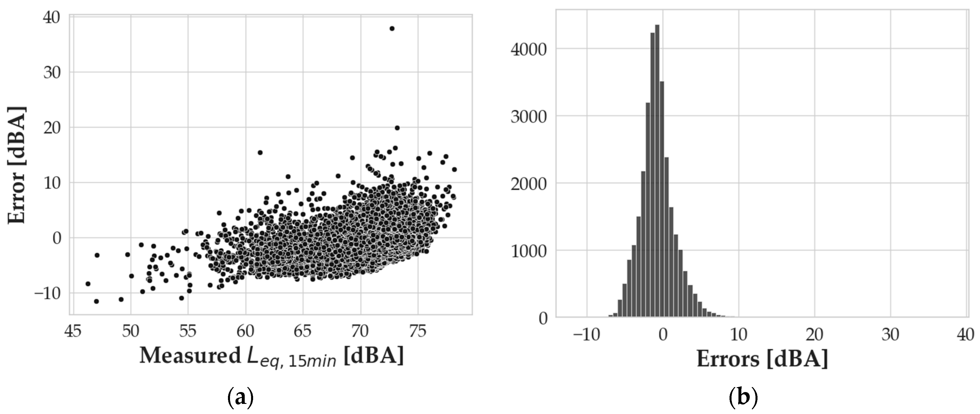
A statistical analysis of the distribution indicates a certain similarity between the distributions, highlighting a slight overestimation of the model. The mean values of the distributions differ for an absolute value of 0.82 dBA and their skewness differs for an absolute value of 0.48. The kurtosis indexes are 4.87 and 2.06 for the measured and computed L_eq,h values, respectively. Error analysis was also performed on the specific application of the model, resulting in Figure 4a, where errors are calculated as the measured L_eq,h minus the simulated L_eq,h.

The cloud of data in the graph in Figure 4a shows that the majority of the errors lie between −5 and +5 dBA, except for some outlier values, especially at high levels of measured L_eq,h. The mean value of the errors is −0.82 dBA, and the standard deviation is 2.25 dBA, while the skewness and kurtosis of the distributions are, respectively, 0.68 and 1.64. The overall error analysis, then, indicates a good-performing model for the case study of the LTMS database.

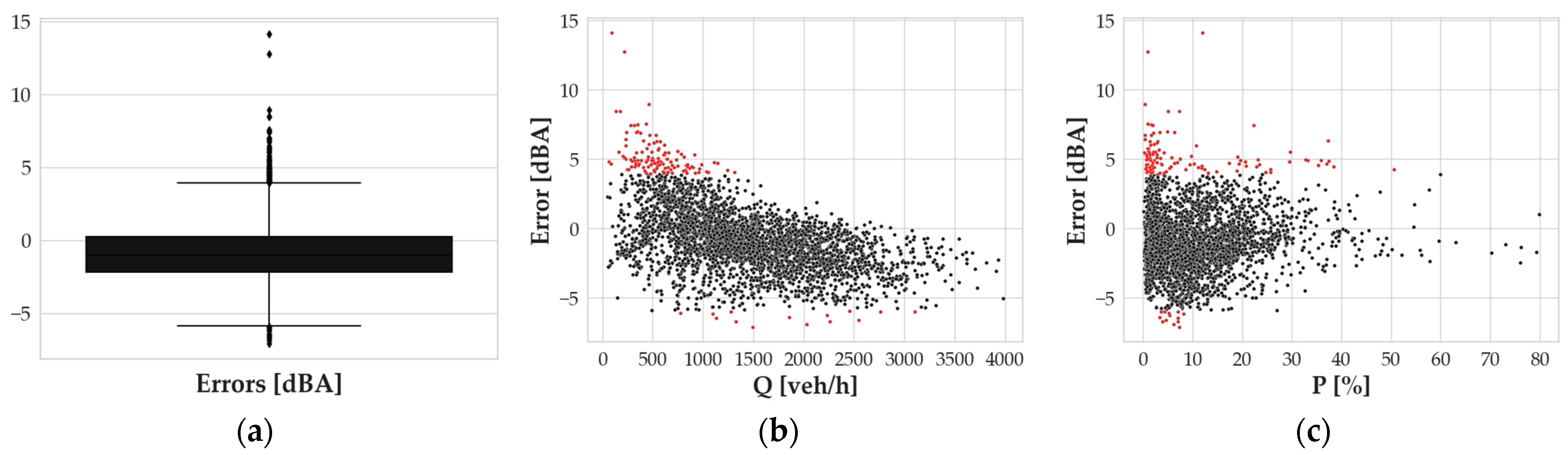
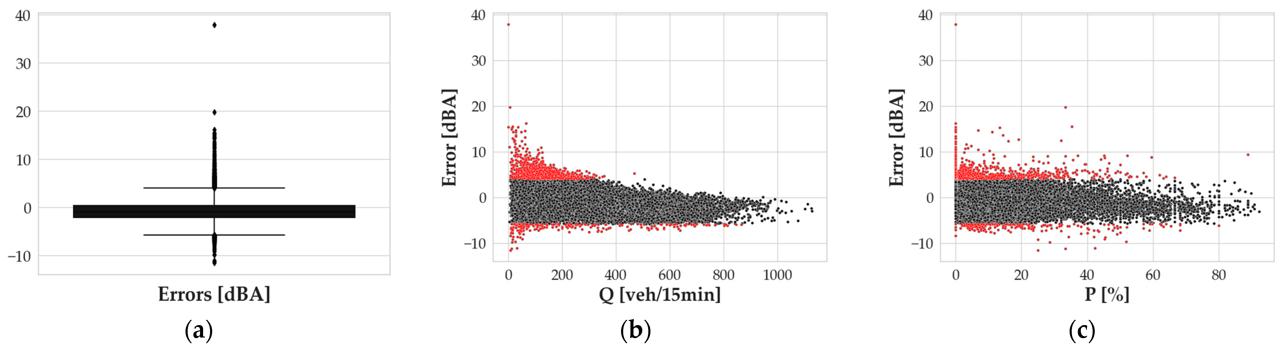
Nevertheless, the authors wanted to deepen the investigation of the performing metrics of the model itself. To do so, the relationship between the error outliers and some specific independent variables was investigated. The investigation was at first carried out using a boxplot analysis (Figure 5a), where the data falling into the interquartile range were represented in the box, and the black diamonds refer to the data falling outside the boundaries of the box ± 1.5 times the interquartile range. The total number of outliers so calculated was 3.93% of the total. These data are also represented by red dots in Figure 5b,c, where error values are represented as a function of Q and P. The outlier data are listed in Appendix A.

As for the graph in Figure 5b, it is clear that the outlier positive values of errors mostly correspond to a low Q value, meaning that the most significant underestimations of the model have to be investigated in periods in which uncommonly high L_eq,h values are associated with a limited amount of traffic. These L_eq,h values are generally related to low P values and high speeds. Such conditions suggest an expectation of values of noise levels lower than those measured (see

Table A1. List of overestimation outlier data.

ID	Leq,h (dBA)	VL (km/h)	VM (km/h)	VH (km/h)	P (%)	Q (veh/h)	Error (dBA)
12	73.47	122.38	85.11	85.11	6.89	508	4.75
221	73.58	101.41	81.26	81.26	19.33	600	4.66
222	74.62	103.98	76.97	76.97	11.10	901	4.43
1165	72.17	120.70	6.00	6.00	0.91	220	12.75
1166	71.80	105.31	90.75	90.75	0.65	619	5.34
1167	72.09	106.02	97.50	97.50	0.30	656	5.50
1168	70.87	102.65	93.00	93.00	1.14	439	5.77
1169	68.28	102.23	92.00	92.00	0.42	236	6.44
1170	73.88	103.55	94.50	94.50	0.43	462	8.95
1171	71.44	104.99	90.50	90.50	1.60	563	4.86
1180	70.43	120.51	83.13	83.13	2.15	325	4.94
1188	72.29	119.09	82.11	82.11	23.16	285	4.99
1190	72.81	115.43	84.67	84.67	1.71	350	7.52
1191	72.75	115.30	90.00	90.00	0.90	558	5.80
1198	73.64	119.97	79.06	79.06	35.92	348	4.94
1199	74.20	117.93	79.01	79.01	25.67	522	4.29
1201	72.98	121.09	79.30	79.30	38.44	320	4.48
1202	73.83	119.65	80.05	80.05	22.93	458	4.48
1245	74.65	117.91	83.83	83.83	0.61	1315	4.08
1246	74.36	119.95	83.83	83.83	1.01	988	4.61
1247	73.78	119.13	88.99	88.99	2.79	610	5.32
1248	73.02	119.93	80.10	80.10	2.17	461	6.10
1249	72.82	118.60	84.88	84.88	3.29	334	6.94
1250	70.16	120.35	81.63	81.63	7.39	230	5.01

in Appendix A). This discrepancy can be related to several reasons; one of them could be the presence of other noise sources occurring during the measurement. Similarly, outliers corresponding to large overestimations are associated with low measured L_eq,h values for the observed flows and speeds. This suggests that some specific situations, not considered in the presented model, could happen during measurements.

The scatterplot of errors vs. P (Figure 5c) represents a similar pattern, and yet, it is more spread over the whole P range. Once they identified the outliers, the authors removed such data and performed a new step of simulation with the “cleaned” dataset to validate the model excluding nonstandard conditions. For the new dataset, the same approach described before was applied by investigating the distributions and the scatterplot of the measured vs. simulated L_eq,h levels reported in Figure 6. A visual comparison between the two histograms is good, and the statistical analyses are comparable: the mean values of the measured and simulated L_eq,h differ in an absolute value of 1.02 dBA; the skewness index of the measured and simulated L_eq,h differs by 0.55, where the kurtosis indexes are now 5.09 and 2.24 for the measured and simulated L_eq,h. The mean and the standard deviations of the error distribution after the removal of the outliers are, respectively, −1.02 dBA and 1.91 dBA, showing a slight worsening of the mean error and a small improvement in the standard deviation with respect to the analysis including the outliers (mean error and standard deviation, respectively: −0.82 dBA and 2.25 dBA). This result confirms that the model can also provide a good average performance when nonstandard conditions of traffic and/or background levels occur.

3.3. Analysis on a 15 Min Timespan

Additional validation of the model’s functioning was performed on the field measurements extracted from the raw LTMS database to evaluate the performance of the model when applied to a set of data provided over 15 min. The choice of applying the model to the same data but with a different timespan thus allowed us to verify the model’s reliability and its usage in situations where an hourly time range is not suitable (for instance, strong variations in the sources) and check the performance of the model using a larger and more detailed set of data.

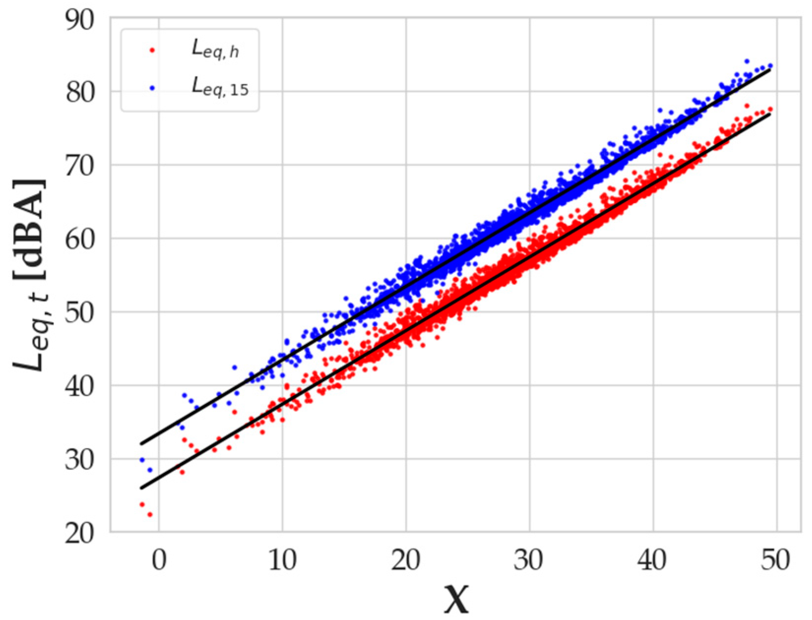
As mentioned in the previous sections, the computed L_eq,h values used for the calibration of the model were obtained with a logarithmic sum where a time-dependent factor was present (1/3600; see Equation (3)). In order to change the timespan to 900 s, a different step of calibration for the model was performed, setting the time factor of Equation (3) to 1/900. The results of the multilinear regression confirm that the L_eq slope lies on the coefficient of the regression, while the intercept accounts for the vertical shift in the simulations (Figure 7). The difference between the intercepts of the two regression lines is 6.02 dBA, which is exactly a result of $10 \log \left(3600/900\right)$, i.e., the conversion from 1 h to 15 min.

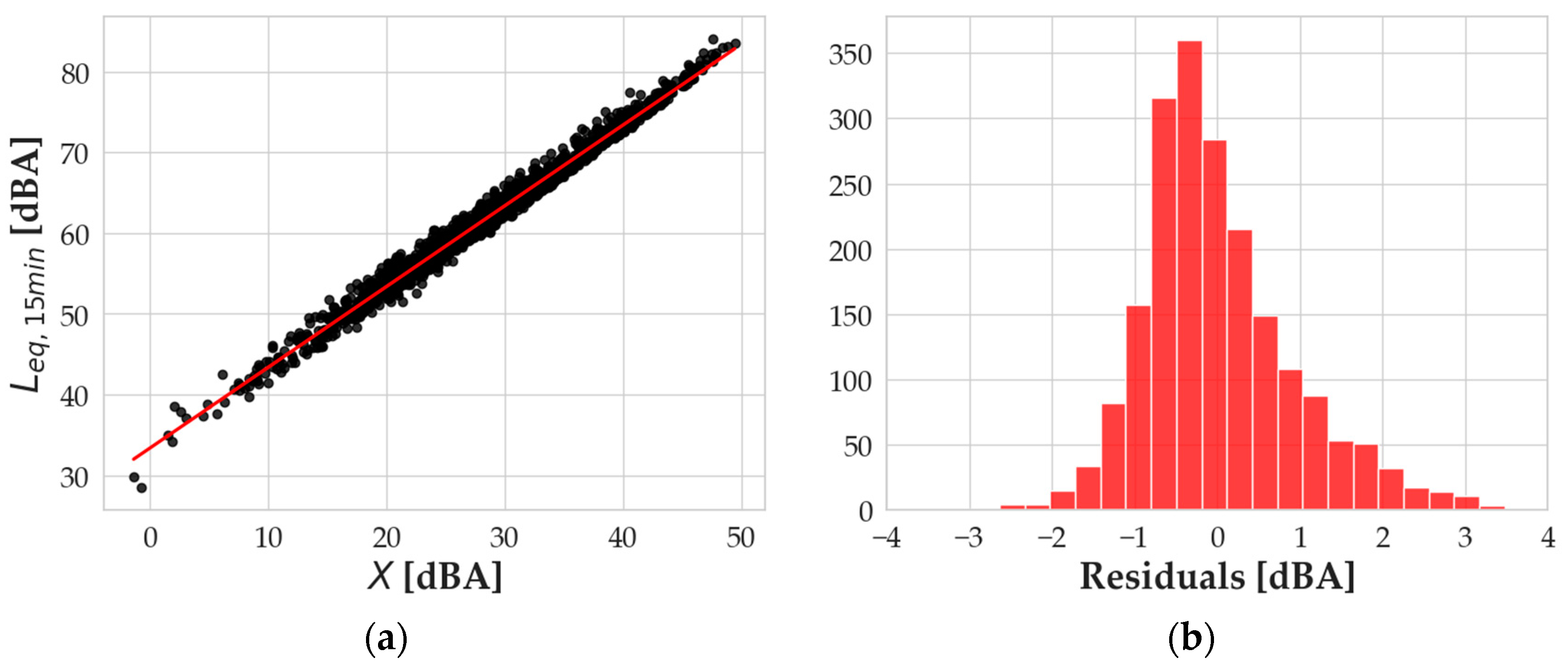
Such an interesting result strongly confirms the possibility of rescaling the computation to any desired time interval, thus adapting to whatever situation needs to be simulated. As for the comparison between the measured and simulated L_eq,15min values, the authors performed the very same approach described above by analyzing the calibration residuals and the validation errors and performing a study on the model performance with and without outlier values. In Figure 8a, the linear regression of the L_eq,15min values vs. the X variable is presented, while in Figure 8b, the distribution of the residuals of the calibration is shown.

Just like the previous application, the residual distribution has a mean value that is basically null (4.3 × 10⁻¹⁴ dBA) and a standard deviation of 0.92 dBA. The kurtosis index is 1.07, making the distribution slightly “leptokurtic”, and the skewness is 0.69, with the right tail more pronounced than the left one. Statistical indexes of residuals, then, are basically equal to the ones obtained when the model was run for L_eq,h, suggesting the goodness of the calibration is independent of the selected timespan.

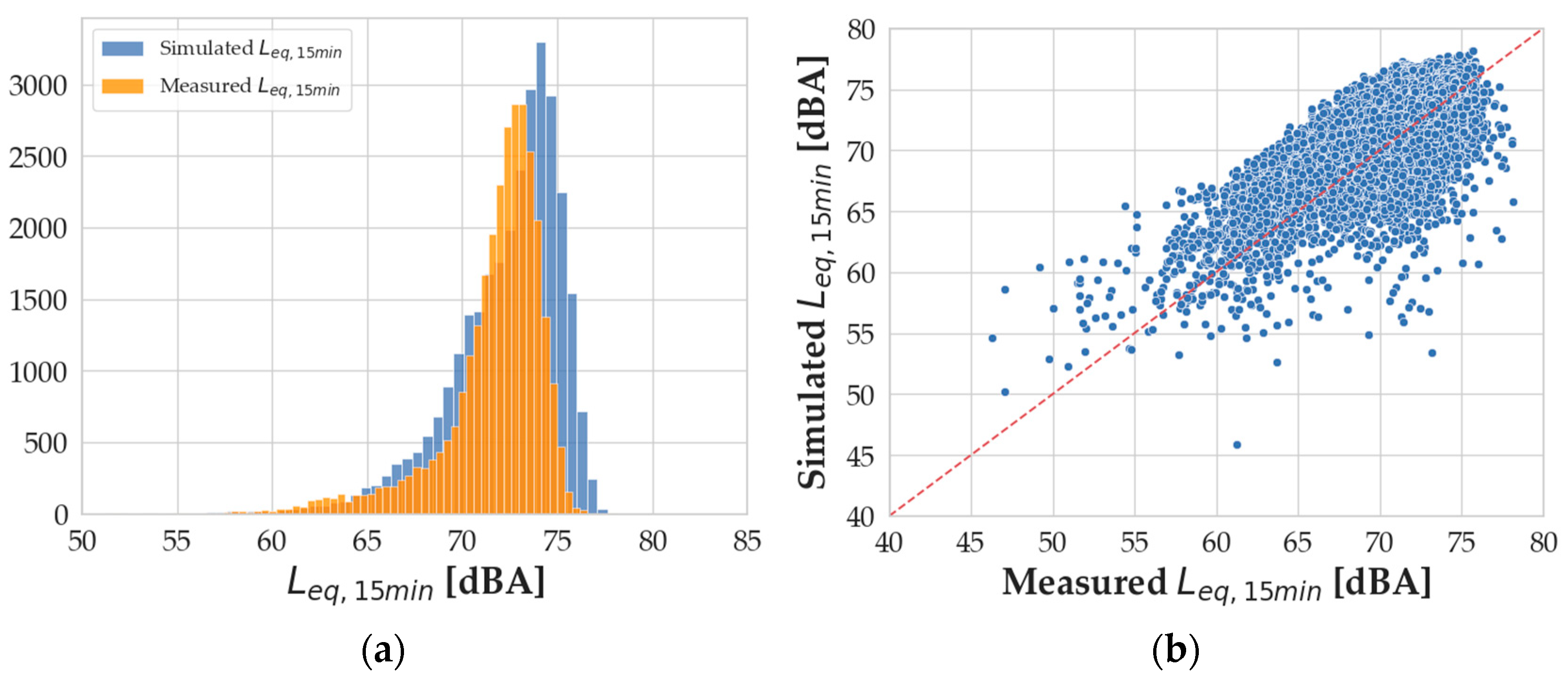
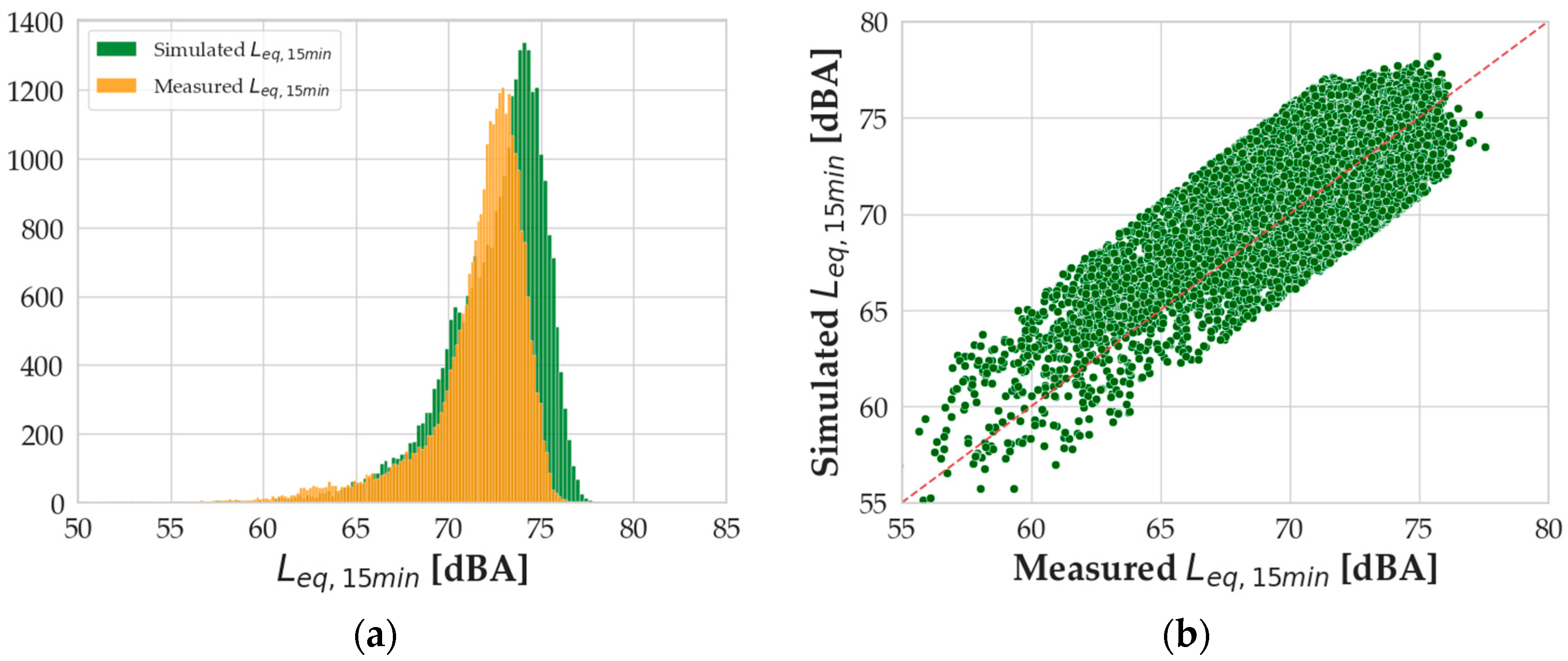
The next step is the validation of the model by using the real traffic data provided by the LTMS database for a 15 min time range and a comparison between the measured and the simulated equivalent levels. In Figure 9, the results are summarized: in the same way as hourly data, the superimposition of the L_eq,15min value distributions shows their similarity, confirmed using statistical indexes. The absolute difference between the mean values is 0.72 dBA. The skewness of the measured L_eq,15min value distribution is −2.04, while the one for the simulated L_eq,15min is −1.52 (absolute difference, 0.51). The kurtosis indexes are 6.11 and 4.24, respectively, for the measured and simulated L_eq,15min value distributions (absolute difference, 1.87).

Figure 10a shows the scatterplot of the validation errors versus the measured L_eq,15min. The error distribution reported in Figure 10b has a mean value of −0.72 dBA and exhibits a quite symmetric shape. The statistical indexes to confirm this visualization are 0.84 for the skewness and 5.11 for the kurtosis.

In performing the outlier analysis, the authors discovered a behavior similar to the one found for the 1 h timespan application of the model. Specifically, outlier values corresponding to the largest errors occurred at low values of Q, as shown in Figure 11b. The error of 37.9 dBA, for instance, corresponds to the measurement performed on 22 September 2004, from 10:30 to 10:45 a.m. In this time slot, the measured L_eq,15min is 72.7 dBA with a total flow of two vehicles over 15 min, one light and one heavy, with a speed of 45 km/h for the light vehicle and 28 km/h for the heavy vehicle. Of course, something occurred in the measurement that is either the presence of an event that altered the noise level measurement or, most probably, a problem in the car counting system.

In general, given the structure of the model, which mimics only the contributions to the noise level from vehicles passing by, when the traffic flow is very small, the background sound level is not negligible.

Following the same approach already described, the authors removed the outliers and performed a new validation process, obtaining the results presented in Figure 12.

The absolute difference in the mean values of the L_eq,15min distributions is now 0.88 dBA; the absolute difference in the skewness of the distributions is now 0.50; and the absolute difference in the kurtosis indexes is 1.88.

Table 3. Statistical values of the distribution of the L_eq,h and L_eq,15min values, with and without outliers.

Distribution	Statistics	Measured	Simulated	Measured without Outliers	Simulated without Outliers
Leq,h	Mean (dBA)	72.1	72.9	72.1	73.1
	Std dev (dBA)	2.0	2.5	2.0	2.6
	Skewness	−1.68	−1.20	−1.72	−1.16
	Kurtosis	4.87	2.07	5.09	2.24
Leq,15min	Mean (dBA)	71.6	72.3	71.6	72.5
	Std dev (dBA)	2.9	3.0	2.8	2.8
	Skewness	−2.04	−1.52	−1.94	−1.44
	Kurtosis	6.11	4.24	5.27	3.39

and

Table 4. Error metrics for 1 h and 15 min timespan datasets, with and without outliers.

Reference Timespan	Error Metrics	Full Dataset	Dataset without Outliers
1 h	Mean error (dBA)	−0.82	−1.02
	Std dev of the error (dBA)	2.25	1.92
	MAE (dBA)	1.90	1.76
	MPE	−1.17%	−1.44%
	MAPE	2.65%	2.46%
15 min	Mean error (dBA)	−0.72	−0.88
	Std dev of the error (dBA)	2.28	1.91
	MAE (dBA)	1.85	1.69
	MPE	−0.36%	−0.76%
	MAPE	2.12%	1.56%

summarize, respectively, the statistical values of the measured and simulated equivalent level distributions and error metrics, with and without outliers. It is possible to see how the statistics of the distributions for the simulation levels are very close to those from the measured distributions, even including outlier data. Similarly, the error metrics are comparable, showing a slight improvement just when the absolute error is considered for the MAE and the MAPE. The removal of outliers, in fact, was not “symmetric” since they were more gathered in the underestimation region; thus, the error metrics that consider the sign of the error tend to move away from zero (see the mean error and MPE in Table 4). On the contrary, the mean absolute error and mean absolute percentage error adopt the absolute value and, thus, decrease thanks to the removal of both high underestimations and overestimations.

Furthermore, the data show that the model output does not have a significant improvement after the removal of outliers, neither for the L_eq,h nor L_eq,15min simulations, suggesting that the model can work properly, on average, when nonstandard conditions occur.

In addition, since all the regulations usually fix limits on day, evening, or night equivalent levels, as well as on entire day levels (L_den), as defined in the European Noise Directive [21], the on-average good performance of the model suggests that this tool can be successfully used to predict these indicators both in proximity to existing road traffic networks and when designing new infrastructures.

4. Conclusions

In this paper, a new model for road traffic noise level assessment was presented. The idea was to build a model with a multilinear regression technique calibrated with computed data rather than measured ones. The implemented formula for computing the L_eq values for the model calibration is simple and versatile since it easily permits to choose a different the Noise Emission Model for the computation of source power levels and provides the opportunity to compute equivalent noise levels over different timespans. The modularity of the choice of the NEM makes the model compatible with any national model and with the EU’s harmonized CNOSSOS framework, also allowing for the inclusion of different propulsion systems, such as electric and hybrid engines, which are more and more present in national fleets. Such a paradigm permitted the creation of a calibration dataset that is as general as possible to cover a multiplicity of traffic flow situations. The random generation of the independent variable values used for the calibration of the model most likely improved this characteristic of the model even more. It is worth noting that the multilinear regression technique allows for the inclusion of different variables according to the situation. All these features make the model usable in a very large number of situations.

A statistical analysis of the residuals of the model in the calibration phase and the errors when validating it with a real dataset allowed us to investigate the model performance as a function of the measured noise levels, total traffic flow, and percentage of heavy vehicles.

The validation was performed also removed unconventional conditions related to traffic and/or the measured levels, thus removing the outliers identified during the analysis. The error metrics confirmed a slight improvement in the absolute errors, although the model also provided average errors lower than 2 dBA, including nonstandard situations. This result is promising since the indicators usually adopted by national regulations are defined by a large time range average, which can be day, evening, or night timespans, as well as full days (L_den). Thus, a model that provides good performance on average is expected to furnish reliable predictions for these time ranges.

The limitations of the model can be highlighted firstly in the use of average speed for the light, medium, and heavy vehicle categories. To achieve a fully dynamic and microscopic model, in fact, the speed of each vehicle is needed. In addition, the presented model assumes that the traffic flows are equally distributed in both direction lanes, resulting in possible underestimation and overestimation during special hours of the day, in which there is a privileged direction of vehicles (for instance, ingoing or outgoing from downtown, respectively, at the beginning and end of working days). To address such limitations, the future steps of this research will be in the direction of the generation of a fully microscopic model, which will take into account the single velocity of each vehicle and its position with respect to the receiver. Finally, as discussed in the outlier analyses, there are possible phenomena that can lead to overestimation or underestimation in the low- and high-value regions of the considered variables. A detailed study of unconventional situations is beyond the scope of this paper and could be a subject of further research, in which the ranges of applicability for the model can be quantitatively estimated.