Abstract
Deep learning plays a highly essential role in the domain of remote sensing change detection (CD) due to its high efficiency. From some existing methods, we can observe that the fusion of information at each scale is quite vital for the accuracy of the CD results, especially for the common problems of pseudo-change and the difficult detection of change edges in the CD task. With this in mind, we propose a New Fusion network with Dual-branch Encoder and Triple-branch Decoder (DETDNet) that follows a codec structure as a whole, where the encoder adopts a siamese Res2Net-50 structure to extract the local features of the bitemporal images. As for the decoder in previous works, they usually employed a single branch, and this approach only preserved the fusion features of the encoder’s bitemporal images. Distinguished from these approaches, we adopt the triple-branch architecture in the decoder for the first time. The triple-branch structure preserves not only the dual-branch features from the encoder in the left and right branches, respectively, to learn the effective and powerful individual features of each temporal image but also the fusion features from the encoder in the middle branch. The middle branch utilizes triple-branch aggregation (TA) to realize the feature interaction of the three branches in the decoder, which enhances the integrated features and provides abundant and supplementary bitemporal feature information to improve the CD performance. The triple-branch architecture of the decoder ensures that the respective features of the bitemporal images as well as their fused features are preserved, making the feature extraction more integrated. In addition, the three branches employ a multiscale feature extraction module (MFE) per layer to extract multiscale contextual information and enhance the feature representation capability of the CD. We conducted comparison experiments on the BCDD, LEVIR-CD, and SYSU-CD datasets, which were created in New Zealand, the USA, and Hong Kong, respectively. The data were preprocessed to contain 7434, 10,192, and 20,000 image pairs, respectively. The experimental results show that DETDNet achieves F1 scores of 92.7%, 90.99%, and 81.13%, respectively, which shows better results compared to some recent works, which means that the model is more robust. In addition, the lower FP and FN indicate lower error and misdetection rates. Moreover, from the analysis of the experimental results, compared with some existing methods, the problem of pseudo-changes and the difficulty of detecting small change areas is better solved.
1. Introduction
Remote image change detection (CD) is the process of obtaining semantic change information such as vegetation and buildings from analyzing multitemporal remote images taken in the same location at different times. Lately, due to the advancement of high-resolution remote images, CD has been broadly employed for disaster monitoring [1,2], in which CD can discover the scope of the damage, so that the rescue and relief personnel can be reasonably arranged and dispatched; urban expansion [3], in which CD can identify alterations in and demolitions of urban buildings and detect the presence of unauthorized buildings; forest and vegetation changes [4], in which CD can effectively identify the growth change areas of forest and vegetation; and many other aspects, which have also attracted more and more scholars to be more interested in this task and to produce a lot of work. The process of CD is shown in Figure 1.
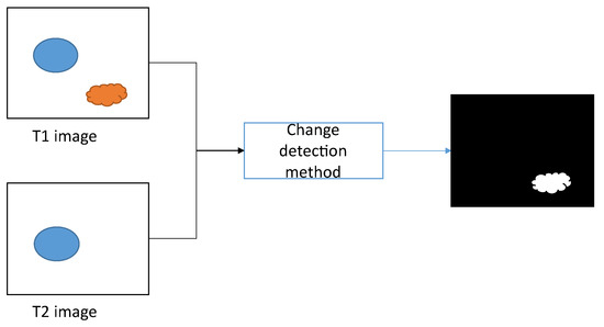
Figure 1.
The process of CD.
Deep learning also has a very promising future in the domain of CD. Owing to the excellent characteristic extraction ability of convolutional neural networks (CNNs), some early CD algorithms have used CNNs to extract bitemporal features [5,6,7,8,9,10,11,12] to complete CD. Zhan et al. [6] established a dual-attention convolutional siamese network, which processed two input images with shared weights and firstly introduced the siamese construction composed of two identical structures in the CD task. However, its loss function only improved the data imbalance and did not effectively solve the problems of pseudo-change and the difficult detection of boundary regions. Daudt et al. [7] first proposed codec-based fully convolutional neural networks (FCNNs), which replaced the fully connected layer with a convolutional layer and could receive inputs of arbitrary size. As none of these methods could obtain the global information of the images due to the local limitations of traditional convolutional feature extraction, some subsequent works made some improvements in this regard as well. Peng et al. [8] put forward the UNet++ Multiple Side-Outputs Fusion network based on UNet++ [13], which fused deep supervision and dense connection mechanisms to optimize the edge details of change regions. In addition, UNet++ consists of different depths of UNet, providing improved segmentation performance for objects of different sizes. Yet, this method ignored the effect of season, light, etc., on change detection. Chen and Shi [10] proposed the pyramid spatial–temporal attention module that modeled the spatial–temporal relationships during the feature extraction phase and considered capturing multiscale spatial–temporal relationships to extract more discriminative features. In [11], a deep-supervised image fusion algorithm was presented to optimize the boundary integrity and compactness inside the target by means of merging multilayer depth features and differential image features. In [12], channel and spatial attention were used when processing images at each moment to obtain more discriminative features. Zhang et al. [9] utilized dilated convolution to enlarge the receptive field, where the dilated convolution was conducted by setting the dilated rate to fill the conventional convolution kernel with 0. Fang et al. [14] adopted UNet++, where features of different levels were closely interconnected in a bottom-up manner to yield fine-grained change maps. These methods somewhat improved the disadvantages of traditional convolution, but they still could not fully extract global information, neither could they accurately identify large-scale objects nor perform well enough to acquire the correlations between the surface objects and the rest of the objects on the entire image.
The Transformer [15] has been gradually applied in the domain of computer vision [16,17,18,19] due to its superior ability to capture long-term dependencies. Similarly, for the purpose of solving the limitations of the CNN mentioned above, the Transformer has made considerable achievements in CD tasks [20,21]. Chen et al. [20] presented a method, where the Transformer was firstly brought into the CD task to enhance the spatial–temporal contextual information extraction capability through the Transformer module, and Were et al. [21] proposed a transformer-based siamese network architecture (abbreviated as ChangeFormer) for CD that united a hierarchical Transformer encoder to generate ConvNet-like multilevel features with a multilayer perceptron (MLP) decoder to effectively extract multiscale long-range relationships. However, these algorithms lacked some capture of local information, and the tight semantic features led to the loss of information such as contour.
Based on the above problems, we realize that both local and global information are important, and the extraction of multiscale features is also an urgent work. SPNet [22] puts forward the feature enhancement and fusion module to fully explore the feature interaction between multimodal information and strengthen the feature communication between different scales, which has made good progress in salient object detection, which is a task to detect the most salient object.
Inspired by SPNet [22], we determined to extend this structure into the field of CD and designed a New Fusion network with Dual-branch Encoder and Triple-branch Decoder (DETDNet). DETDNet adopts a codec architecture. The encoder is a dual-branch siamese structure, and the bitemporal image features are fused by a concise but effective module, namely concatenation and a convolution operation (CAC). Moreover, the decoder uses a triple-branch structure, while using a refined Receptive Field Block (RFB) improved from [23,24] to extract the multiscale contextual characteristics of the three branches, denoted as the multiscale feature extraction module (MFE), and to fuse the features of each layer in the middle branch with the next layer via the triple-branch aggregation (TA) module. Finally, the resolutions of the three change maps are recovered to be in accordance with the raw images after upsampling, and these three change maps are fused to build the final change map we need.
The key work of this article unfolds in three ways:
(1) DETDNet is proposed, in which the encoder is a dual-branch structure that captures the local features of images, and for the first time, a three-branch structure is used in the decoder to obtain multiscale features by using MFE.
(2) We use different feature fusion methods for the decoder and encoder, respectively. The encoder applies CAC to fuse the bitemporal images taken in the same location at different times, and the decoder uses the TA module to fuse the triple-branch features. Futhermore, a cascade operation is adopted to fuse the features from the same stage in the encoder and decoder.
(3) The experiments implemented on three publicly available datasets demonstrate our approach exceeds some recent approaches in terms of the F1 score, IoU, and OA.
2. Related Work
2.1. CNN-Based Network
Deep learning is being broadly employed in CD tasks due to its potent ability to process computer vision tasks. Among them, the powerful feature representation capability of CNN enables it to play a great role in early CD. Zhan et al. [6] framed a two-branch structure with shared weights, and the difference image of the input images could be obtained by calculating the feature maps output from the two-branch network with Euclidean distance. Weighted contrastive loss was used to distinguish the changed pixels from the unchanged pixels more effectively, so as to reduce the influence of data imbalance. However, the network was not well altered to effectively extract image features, and the small sample of datasets used was not convincing enough to perform comparison experiments. Daudt et al. [7] brought fully convolutional into the CD domain by proposing three CD algorithms, namely the FC-EF, FC-Siam-conc, and FC-Siam-diff. The FC-EF is an early fusion-based model that concatenates bitemporal images along the channel dimension and later passes them into a fully convolutional network, while the other two, FC- Siam-conc and FC-Siam-diff, are siamese architectures. Moreover, the models achieved better performance than the previously proposed methods, while being at least 500 times faster than related systems. Similarly, these networks are not a good solution to the problem of pseudo-change and small change targets that are difficult to detect. Aiming to solve the circumstance of pseudo-change and the difficult detection of change edges in remote sensing image CD, much recent research has been directed to the strategy of feature fusion. STANet [10] designed a siamese neural network through obtaining illumination invariance and misalignment robustness features, but the proposed BAM and PAM only considered the spatial attention weights between bitemporal images. Zhang et al. [11], using dual branches, presented a depth-supervised strategy to optimize the change boundary by means of merging multilayer deep features and differential image features. In addition to this, various works have been conducted by researchers to expand the receptive field, such as the use of atrous convolution [25] and the use of various attention mechanisms. SNUNet [14] presented a dense connection network based on UNet++ that incorporated multiscale features, and finally, the ECAM module enhanced the feature representation by an attention mechanism [26]; however, ECAM only employed a channel attention mechanism and ignored spatial relations. Liu et al. [12] described a dual-attention module to obtain both the spatial and channel attention at the same time.
Although a growing number of CNN-based works consider CD from the perspective of multiscale feature fusion, these works still lack the modeling of global contextual features; therefore, we remedy this shortcoming in our work.
2.2. Transformer-Based Network
Given the predominance of the Transformer in modeling long-range dependencies, it has also been applied to CD tasks in recent years. A bitemporal image Transformer network (BiT) was put forward in [20], in which the Transformer was firstly applied in the domain of CD. The BiT effectively modeled contextual information in the token-based spatial–temporal, and context-rich tokens were used to boost the original features. This method takes into account the influence of pseudo-change on the change detection results. Nevertheless, the BiT ignored the utilization of multiscale features. A Transformer-based siamese network was later presented in [21], which efficiently extracted multiscale long-range information by combining a hierarchical Transformer encoder well as a simple MLP decoder to locate the change location more precisely. Nevertheless, Changeformer did not have an advantage in terms of computation.
Based on the above presentation and analysis of some of the previous works, we propose DETDNet, a model to compensate for the shortcomings of the above works, mainly including the effect of pseudo-change on the CD results, the detection of small target objects, the detection of change boundaries, etc. The model achieves a good tradeoff in performance and computation. The network presented in this article is described in detail in the next section.
3. Methodology
In this section, we demonstrate the general framework of DETDNet first, followed by a detailed description of the encoder structure and then the decoder. The MFE module is then shown in Section 3.4. Finally, two different feature fusion modules are provided, one for the encoder and another for the decoder.
3.1. Overview
The DETDNet presented in this article involves a dual-branch input and a triple-branch output. The model diagram, as depicted in Figure 2, employs a U-shaped structure overall. More detailed internal implementation of the encoder and decoder are revealed in Figure 3 and Figure 4. Initially, the bitemporal images are input into a dual-branch encoder to obtain multilevel local feature representations, where the feature representations of each level are fused by CAC. In addition, the original features of each layer from the encoder are aggregated to the corresponding layer of the decoder by a skip connection. The decoder adopts a triple-branch structure, which extracts the multiscale contextual features using MFE and aggregates the features extracted by the MFE from the three branches using the proposed TA module at each layer of the decoder. The concrete details of each module are elaborated as follows.
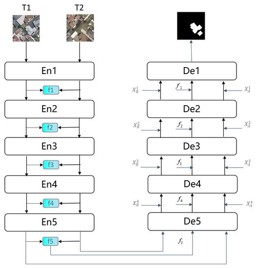
Figure 2.
Overview of DETDNet.
3.2. Encoder
As shown in Figure 3, we used Res2Net-50 [27] to construct the encoder, used for local feature extraction, and pretrained it first on the ImageNet [28] dataset. Given the aligned original input images T1 and T2, both of size , T1 and T2 passed through 5 stages (En1, En2, En3, En4, and En5, respectively) to obtain the multiscale feature representations, respectively. Here, the multiscale feature maps output after 5 stages of encoder are expressed as and , i means the ith layer, and . Their sizes were 1/4, 1/4, 1/8, 1/16, and 1/32 of the original size, respectively, and the channels were 64, 256, 512, 1024, and 2048. The and obtained from each level were fused to output the corresponding through a simple but effective CAC module, and the specific output sizes of each stage are shown in Table 1. Owing to local correlation and translational invariance, traditional CNNs can effectively model local fine-grained information using prior information [29].

Table 1.
Encoder output feature size for each stage.

Figure 3.
The structure of the encoder.
3.3. Decoder
As shown in Figure 4, the work in this paper adopted a triple-branch structure in the decoder for the first time, where the left and right branches represent the feature decoding process of T2 and T1, respectively, and the middle branch represents the feature fusion of T2 and T1.
(1) Left and right branches: The left and right branches of the decoder each included five stages. In the former four stages, each one consisted of an MFE module and a concatenation operation. The last stage was composed of three parts, namely the MFE, convolution, and the upsampling operation. Taking the left branch as an example, the feature generated from the last stage of the encoder was put into the MFE module to produce a feature, represented by . In addition, to better integrate the multilevel features and fuse the local features with multiscale contextual information, a skip connection was built, located between the encoder and decoder, that is, for and after upsampling to perform concatenation operation along the channel dimension, and we denote the obtained features by . The concrete process of the first 4 stages is shown as follows:
In the last stage, went through an MFE, after which the output features underwent a convolution for channel dimension reduction; finally, the feature map size was recovered to be in accordance with the raw image employing a bilinear interpolation upsampling operation.

Figure 4.
The structure of the decoder.
(2) Middle branch: Similarly, the middle branch was divided into 5 stages, the first 4 of which were the same, each of which contained an MFE, TA, and a concatenation operation. The last stage was the same as the left and right branches. In the first four stages, taking the first stage as an example, the two-branch fusion feature generated by CAC from the encoder last stage passed through an MFE block, and the feature was represented by . Together with the output and of the same stage of the left and right branches, they were first upsampled and then sent to a TA block to fuse three-branch features. Finally, the from the encoder performed a concatenation operation with the three-branch fused features through a skip connection for the purpose of combining local and more global information. The first 4 stages of the process are specified as follows:
The feature maps’ sizes from every stage in the decoder are shown in Table 2.
Table 2.
Decoder output feature size for each stage.
3.4. MFE
Motivated by [23], we employed an MFE module at each layer of the decoder, as displayed in Figure 5. The MFE added a branch on the basis of the original RFB [22] module to enlarge the receptive field even more and added an asymmetric convolution layer [30] on top of the RFB-s to extract more discriminative features and enhance the robustness of the model without increasing the computational effort. On the side, a channel attention mechanism (CAM) [25] was added. In the MFE, firstly, a convolution was chosen to shorten the channels to 32 to speed up the inference, and the output features are indicated by , where . Next, for the second, third, and fourth branches, the original features were fed into three convolutional layers, successively, once again after the convolution in the first layer, with convolutional kernel sizes of , , and , after which the features extracted from the corresponding branch were output. After obtaining the features of the five branches, the first four branches were concatenated, whereafter, there was a convolution operation. The was obtained by summing the features of the fifth branch, multiplying the by the attention weights obtained by the CAM, and then summing them again, after an activation function to obtain the final MFE output. The overall process of the MFE is shown in the following equations:
where is the output feature of each branch, and Y is the final output of the MFE.
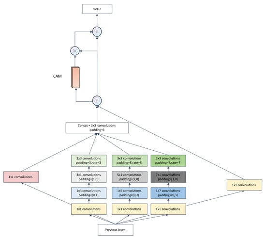
Figure 5.
The structure of the MFE.
3.5. Feature Fusion Module
In CD tasks, there are different forms of bitemporal feature fusion; Fang et al. [14] used simple channel concatenation in the decoder, and Lan et al. [31] studied difference maps using pixel-wise subtraction. As for the decoder, channel concatenation is commonly used for fusing features at the same layer of the encoder and decoder. However, simple channel concatenation, subtraction, and element-wise summation do not effectively explore the relationship between bitemporal images and do not achieve the interaction between channels well. In view of this, this paper adopted different feature fusion approaches in the encoder and decoder stages.
For the encoder phase, we first concatenated the bitemporal features along the channel dimension, and then the concatenated features underwent a CNN block, which mainly contained a convolution, BN, and ReLU. The CNN block here could significantly strengthen the nonlinear representation of the network, in addition to reducing the dimensions of the features and realizing the mutual information effect between channels for fusion with the same-layer features in the decoder.
For the purpose of fully exploiting the relationship between the bitemporal features, a new module TA was introduced in the decoder, as shown in Figure 6. The left, right, and middle are the features of each layer of the decoder after the MFE, where the left is the left branch, which corresponds to the T2 image branch of the encoder, the right is the right branch, which corresponds to the T1 image branch of the encoder, and the middle corresponds to the T1 and T2 fusion feature branch of the encoder. Particularly, we used the left and right branch features to enhance the fusion features of the middle branch. The specific operations were as follows: Firstly, the left and right moved through a spatial attention module (SAM) [25], respectively, and the two output attention maps were then multiplied by the original middle branch for adaptive feature refinement. Secondly, the two obtained outputs were channel concatenated, and the obtained outputs were finally combined with the original middle fusion features through a summation operation, followed immediately by a convolution for the fusion features to avoid the aliasing effect introduced by element-wise summation.
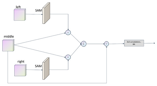
Figure 6.
The structure of the TA.
4. Experiments
To confirm the superiority of this method, we executed experiments on the BCDD [32], LEVIR-CD [10], and SYSU-CD [33] datasets, and a sequence of comparative experiments was designed to compare this model with some classical models from recent years. To be fair, the experimental settings were conducted according to the original article.
4.1. Datasets
The BCDD dataset was collected in New Zealand and covered Christchurch. It contains two high-resolution remote sensing images with a registration error of 1.6 pixels. The imaging dates were 2012 and 2016, respectively, the resolution is 0.3 m/pixel, and the size is 32,507 × 15,354 pixels. To make the training more convenient, we cropped the images into non-overlapping 256 × 256 image pairs, for a total of 7434 pairs, and divided them randomly in the ratio of 8:1:1 into a training set, validation set, and testing set.
The LEVIR-CD dataset originated from the Beihang LEVIR team, and the imaging locations were 20 different areas in several cities in Texas, USA. The imaging time varied from 2002 to 2018. Over 31,000 individual instances of change were fully labeled in 637 image pairs of 1024 × 1024 pixels and a resolution of 0.5 m, among which the change in land use types such as urban expansion was more significant. For the convenience of training, we cropped the image into small nonoverlapping blocks of 256 × 256 pixels, and the dataset was randomly partitioned, with 7120 image pairs as the training set, 2048 image pairs as the validation set, and 1024 image pairs as the testing set.
The SYSU-CD dataset includes 20,000 pairs of 0.5 m aerial images collected in Hong Kong in 2007 and 2014. The primary change types in the dataset comprised suburban sprawl, new urban construction, pre-construction groundwork, road expansion, vegetation changes, and marine construction. In this experiment, we partitioned the whole dataset into a training set, a validation set, and a testing set in the proportion of 6:2:2.
Table 3 shows the sizes of the three datasets used.
Table 3.
Detailed information of the three datasets.
4.2. Implementation Details
For this experiment, pytorch was used as the training framework. For the convergence acceleration of the model, Res2Net-50 [27] was pretrained on the ImageNet [28] dataset to initialize the parameters of DETDNet. The training batch size was set to 16, the optimizer was Adam, the initial learning rate was set to 0.001, and the model was iterated for 100 epochs, with the learning rate decaying by 0.5 for every eight epochs. The specific hardware configuration was an NVIDIA TITAN RTX (24 GB) GPU.
4.3. Evaluation Metrics
Considering that the remote sensing CD task can be seen as a binary classification task, the precision, recall, F1 score, intersection over union (IoU), and overall accuracy (OA) were selected as the evaluation metrics to quantitatively validate the efficiency of the algorithm presented in this article. These evaluation metrics are always used to measure binary classification models in machine learning. The expressions of these evaluation metrics are listed below:
denotes the sum total of the changed pixels predicted to be changed, denotes the total number of unchanged pixels predicted to be changed, denotes the total number of unchanged pixels predicted to be unchanged, and denotes the total number of changed pixels predicted to be unchanged.
4.4. Performance Comparison
To prove the superiority of the method put forward in this article, DETDNet was compared with some advanced methods in current CD tasks, including FC-EF [7], FC-Siam-conc [7], FC-Siam-diff [7], CDNet [34], STANet [10], BiT [20], SNUNet [14], and ChangeFormer [21]. To be fair, we conducted comparative experiments in the same environment, that is, the same software environment, hardware environment, and dataset processing methods.
4.4.1. Comparative Experiments on the BCDD Dataset
We display the quantitative experimental results of various algorithms on the BCDD dataset in Table 4. The results in the table reveal that our algorithm achieved 93.84%, 91.59%, 92.70%, 86.40%, and 99.32% for the precision, recall, F1 score, IoU, and OA, respectively, which were higher than all the other methods and 3.3%, 5.56%, and 0.2% over the second-best method on the main metrics of the F1 score, IoU, and OA, respectively. The highest precision and recall also indicate that our model is more robust compared to the other methods. The above results proved the method in this article surpasses these comparative methods. Figure 7 illustrates the visualization results of the comparative experiments performed on the BCDD dataset. For easier observation, the , , , and are marked in the figure with white, black, red, and green, respectively. It is obvious that our model can avoid the and more effectively than other methods. The first and third rows show that the comparison methods had poorer detection accuracy for the change edges, leading to boundary misses or misdetections, thus making the boundary more blurry, while our method detected clearer boundaries, probably due to our TA module, which can efficiently extract the spatial relationships between bitemporal features. As viewed from the second and fourth rows, the influence of the land cover and color around the building in the bitemporal images caused the comparison methods to easily detect the non-changing areas as changing areas. By contrast, the proposed method in this paper circumvented this drawback. This is mainly due to the MFA module. By increasing the receptive field, the MFA module can obtain more global feature relationships and enhance the extraction of semantic information, thus reducing the influence of the pseudo-changes on the CD results. Moreover, due to the use of the dilated convolution and strip convolution, our method is superior to the second-best model in terms of the number of parameters.
Table 4.
Comparison results on the BCDD Dataset.
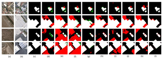
Figure 7.
Visualization results of several CD methods on the BCDD dataset. (a) T1 images. (b) T2 images. (c) Ground truth. (d) FC-EF. (e) FC-Siam-conc. (f) FC-Siam-diff. (g) CDNet. (h) STANet. (i) BIT-CD. (j) SNUNet. (k) ChangeFormer. (l) DETDNet.
4.4.2. Comparative Experiments on the LEVIR-CD Dataset
The quantitative results of the comparison experiments conducted on another public dataset LEVIR-CD are exhibited in Table 5. As Table 5 shows, our algorithm was significantly better than the rest of the algorithms in the main metrics of performance, the F1 score, IoU, and OA, and was 0.82%, 1.37%, and 0.06% better than the second best algorithm, respectively. Figure 8 depicts the visualization results of the comparison experiments. As the spectral information of the images taken at different times may be different, it may cause misdetections or missing detections; as shown in the first line, with respect to the changed area at the bottom right corner, because of the influence of the spectral information, some other methods showed red and some showed green, while our method detected the changed area more accurately. As seen in lines 2 and 7, our method detected both large target regions and small change regions relatively accurately, due to the proposed idea of combining the local features from the encoder as well as the more global features from the decoder. In lines 3, 4, 5, and 6, the shadowed parts of the images caused the comparison methods to easily detect non-changing regions as changing regions; however, our method successfully avoided such pseudo-change.
Table 5.
Comparison results on the LEVIR-CD dataset.
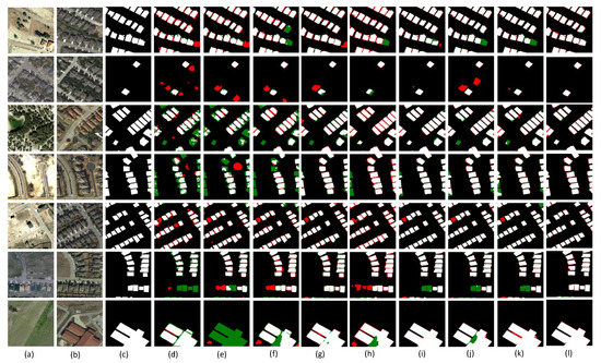
Figure 8.
Visualization results of several CD methods on the LEVIR-CD dataset. (a) T1 images. (b) T2 images. (c) Ground truth. (d) FC-EF. (e) FC-Siam-conc. (f) FC-Siam-diff. (g) CDNet. (h) STANet. (i) BIT-CD. (j) SNUNet. (k) ChangeFormer. (l) DETDNet.
4.4.3. Comparative Experiments on the SYSU-CD Dataset
The quantitative results of all kinds of comparison methods with DETDNet performed on the SYSU-CD dataset are exhibited in Table 6. As displayed in Table 5, our model outperformed the second highest model in the F1 score, IoU, and OA by 1.41%, 1.98%, and 0.71%, respectively. As for the visualization results, they are presented in Figure 9. The main changes in rows 1, 2, 3, 4, and 6 were the building expansions. It can be seen that whether it was the new buildings around the vegetation in rows 1 and 2, the expansion of the seaside buildings in row 3, or the building expansions around the highway in rows 4 and 6, our model was better able to handle the change boundaries and obtain more accurate boundaries. For the change area in the middle of row 2 and the color change of the building roof in row 4, our model recognized the pseudo-change due to the color better. For the change type of vegetation in rows 2 and 5, we can see that our model also had better prediction results. From a comprehensive point of view, since the scenes in the SYSU-CD dataset were relatively complex, there may be various types of changes in the single image, which makes it more difficult to detect, and our model was comparatively better at extracting the features of the different changes and arriving at a more accurate change map.
Table 6.
Comparison results on the SYSU-CD dataset.
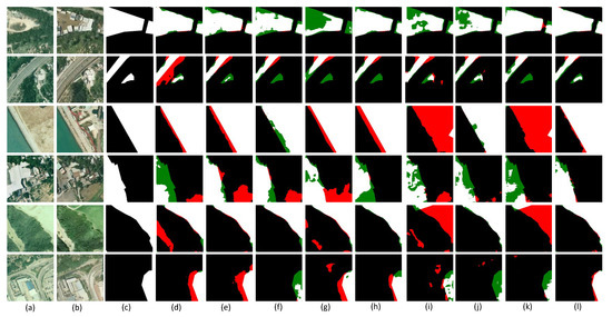
Figure 9.
Visualization results of several CD methods on the SYSU-CD dataset. (a) T1 images. (b) T2 images. (c) Ground truth. (d) FC-EF. (e) FC-Siam-conc. (f) FC-Siam-diff. (g) CDNet. (h) STANet. (i) BIT-CD. (j) SNUNet. (k) ChangeFormer. (l) DETDNet.
4.5. Ablation Experiments
We conducted ablation experiments mainly on the BCDD and LEVIR-CD datasets to determine the improvement in each part of the model, which were mainly divided into the following four aspects.
4.5.1. Effectiveness of the Pretraining
Before training, we first initialized the weight parameters using Res2Net-50 [27] pretrained on the ImageNet [28] dataset, with the pretrained model provided by Res2Net-50 [27]. To demonstrate the necessity of pretraining, the ablation experiment was conducted on the BCDD dataset. Moreover, the results are tabulated in Table 7, where × indicates no pre-trained and √ indicates pre-trained. From the visualization results in Figure 10, it is noticeable that the metrics were significantly lower without pretraining than with pretraining, based on which the necessity of pretraining is confirmed.
Table 7.
The effect of pretraining.
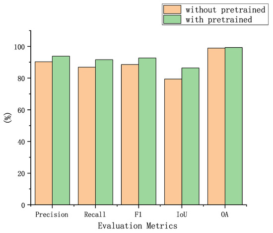
Figure 10.
Visualization results of the impact of pretraining.
4.5.2. The Selection of the Feature Fusion Method
As described above, different feature fusion methods were used between the branches within the encoder and decoder, where the encoder used the CAC to fuse the dual-branch features, and the decoder used the TA to aggregate the triple-branch features. To confirm the adaptability of the two fusion methods in the encoder and decoder, this paper tried to use the TA in the encoder and the CAC in the decoder, based on which ablation experiments were implemented on the BCDD dataset. Table 8 includes the results, which shows that the effect of using the TA in the encoder was somewhat lower than that of the original fusion mode in the F1 score, IoU, and the OA. In addition, we changed the TA in the decoder to the CAC, and Table 9 lists the results, whose performance was also reduced as opposed to the original TA fusion method. In the encoder stage, using the CAC can simply and effectively fuse the dual-temporal features, while using the TA module will cause the redundancy of features. In the decoder stage, on account of the integration of local and multiscale contextual features, the features are relatively more complex, and for the fusion of the left and right branches and the middle branch, using the TA can extract the change features more accurately.
Table 8.
Impact of the feature fusion method in the encoder.
Table 9.
Impact of the feature fusion method in the decoder.
4.5.3. Impact of the MFE
The model in this paper used a modified RFB module, which we referred to as an MFE. According to [30], the MFE has a stronger feature representation, and the model is more robust compared to the original RFB [24] and RFB-s [24]. For this reason, the related ablation experimental results rendered on the LEVIR-CD dataset are provided in Table 10. The setup of the specific ablation experiments was that the MFE module in the decoder was replaced by an RFB and RFB-s, respectively, which are also used for extracting multiscale contextual features. The metrics of the MFE module were remarkably higher than those of RFB and RFB-s, except for the recall, which was slightly lower than those of RFB and RFB-s.
Table 10.
Impact of the MFE.
4.5.4. The Importance of Each Branch of the MFE
We performed a variety of experiments on the BCDD to determine the implications of each branch in the MFE on the model as a whole. The MFE contained a total of five branches, and in the experimental setup, four of them were kept unchanged and branches 0, 1, 2, and 3 were removed in turn. This operation was executed to demonstrate the importance of extracting multiscale contextual features. The resulting data in Table 11 imply that the model yielded better performance than the rest of cases when the MFE was used. Moreover, Figure 11 shows the trend of the F1 score at various settings in the training process.
Table 11.
Importance of each branch of the MFE.
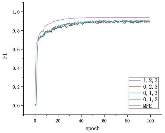
Figure 11.
Visualization results for the importance of each branch in the MFE.
5. Conclusions
The model in this paper is designed to focus on remote sensing image change detection. The model uses a dual-branch structure in the encoder to extract local features, a triple-branch structure in the decoder to extract more global contextual information, and a TA module to effectively fuse the left and right branches with the middle branch. We validated the performance of the DETDNet on the SYSU-CD, LEVIR-CD, and BCDD datasets. In the three datasets, our model reached the optimal value in the F1 score, OA, and IoU. Among them, in the BCDD dataset, our F1 score, OA, and IoU were 3.3%, 0.2%, and 5.56% higher than the second best method, respectively. In the LEVIR-CD dataset, our model outperformed the next best method by 0.82%, 0.06%, and 1.37%, respectively. In the SYSU-CD dataset, our model was 1.41%, 0.71%, and 1.98% higher than the second best method, respectively. The BCDD dataset mainly contains large sparse buildings, and the LEVIR-CD contains small dense buildings. However, both contain pseudo-changes, and the data volume is relatively small compared to the SYSU-CD. These two datasets test the model’s ability to learn and explore potential relationships with a small amount of data. The SYSU-CD has a large amount of data but not high labeling accuracy, which tests the model’s generalization ability. In addition to this, we conducted four sets of ablation experiments to prove the significance of each component in the model. Although the receptive field was increased by the MFA module, the maximum receptive field was 23 after calculation. Therefore, it can be seen that the global features cannot be fully obtained in the shallow layers. Based on this, our subsequent work will focus on using the Transformer or MLP to obtain the global features to achieve a higher performance.
Author Contributions
Conceptualization, C.Z.; methodology, J.Y. and C.Z.; software, C.Z.; validation, L.W., C.Z. and J.Y.; formal analysis, L.W.; resources, L.W.; data curation, C.Z.; writing—original draft preparation, C.Z.; writing—review and editing, L.W.; visualization, L.W.; supervision, L.W. All authors have read and agreed to the published version of the manuscript.
Funding
This research was funded by the National Science Foundation of China under Grant U1903213 and the Scientific and Technological Innovation 2030 Major Project under Grant 2022ZD0115802.
Data Availability Statement
The BCDD, LEVIR-CD, and SYSU-CD datasets are openly available at http://gpcv.whu.edu.cn/data/building_dataset.html (accessed on 30 March 2023), https://justchenhao.github.io/LEVIR/ (accessed on 30 March 2023), https://mail2sysueducn-my.sharepoint.com/personal/liumx23_mail2_sysu_edu_cn/_layouts/15/onedrive.aspx?ga=1 (accessed on 30 March 2023), respectively.
Conflicts of Interest
The authors declare no conflict of interest.
Abbreviations
The following abbreviations are used in this manuscript:
| CNN | convolutional neural network |
| RS | remote sensing |
| CD | change detection |
| FCNNs | fully convolutional neural networks |
| FC-EF | fully convolutional early fusion |
| FC-Siam-conc | fully convolutional siamese concatenation |
| FC-Siam-diff | fully convolutional siamese difference |
| STANet | spatial–temporal attention-based network |
| BiT | bitemporal image Transformer |
| SNUNet | a combination of siamese network and NestedUNet |
| ChangeFormer | a Transformer-based siamese network architecture for change detection |
| ReLU | rectified linear unit |
| DETDNet | a new fusion network with dual-branch encoder and triple-branch decoder |
| MFE | multiscale feature extraction |
| TA | triple-branch aggregation |
| CAC | concatenation and convolution |
| SAM | spatial attention module |
| CAM | channel attention module |
| IoU | intersection over union |
| OA | overall accuracy |
References
- Vetrivel, A.; Gerke, M.; Kerle, N.; Nex, F.; Vosselman, G. Disaster damage detection through synergistic use of deep learning and 3D point cloud features derived from very high resolution oblique aerial images, and multiple-kernel-learning. ISPRS J. Photogramm. Remote Sens. 2018, 140, 45–59. [Google Scholar] [CrossRef]
- de Alwis Pitts, D.A.; So, E. Enhanced change detection index for disaster response, recovery assessment and monitoring of accessibility and open spaces (camp sites). Int. J. Appl. Earth Obs. Geoinf. 2017, 57, 49–60. [Google Scholar] [CrossRef]
- Huang, X.; Zhang, L.; Zhu, T. Building change detection from multitemporal high-resolution remotely sensed images based on a morphological building index. IEEE J. Sel. Top. Appl. Earth Obs. Remote Sens. 2013, 7, 105–115. [Google Scholar] [CrossRef]
- Desclée, B.; Bogaert, P.; Defourny, P. Forest change detection by statistical object-based method. Remote Sens. Environ. 2006, 102, 1–11. [Google Scholar] [CrossRef]
- Chen, J.; Yuan, Z.; Peng, J.; Chen, L.; Huang, H.; Zhu, J.; Liu, Y.; Li, H. DASNet: Dual attentive fully convolutional Siamese networks for change detection in high-resolution satellite images. IEEE J. Sel. Top. Appl. Earth Obs. Remote Sens. 2020, 14, 1194–1206. [Google Scholar] [CrossRef]
- Zhan, Y.; Fu, K.; Yan, M.; Sun, X.; Wang, H.; Qiu, X. Change detection based on deep siamese convolutional network for optical aerial images. IEEE Geosci. Remote Sens. Lett. 2017, 14, 1845–1849. [Google Scholar] [CrossRef]
- Daudt, R.C.; Le Saux, B.; Boulch, A. Fully convolutional siamese networks for change detection. In Proceedings of the 2018 25th IEEE International Conference on Image Processing (ICIP), Athens, Greece, 7–10 October 2018; IEEE: Piscataway, NJ, USA, 2018; pp. 4063–4067. [Google Scholar]
- Peng, D.; Zhang, Y.; Guan, H. End-to-end change detection for high resolution satellite images using improved UNet++. Remote Sens. 2019, 11, 1382. [Google Scholar] [CrossRef]
- Zhang, M.; Xu, G.; Chen, K.; Yan, M.; Sun, X. Triplet-based semantic relation learning for aerial remote sensing image change detection. IEEE Geosci. Remote Sens. Lett. 2018, 16, 266–270. [Google Scholar] [CrossRef]
- Chen, H.; Shi, Z. A spatial-temporal attention-based method and a new dataset for remote sensing image change detection. Remote Sens. 2020, 12, 1662. [Google Scholar] [CrossRef]
- Zhang, C.; Yue, P.; Tapete, D.; Jiang, L.; Shangguan, B.; Huang, L.; Liu, G. A deeply supervised image fusion network for change detection in high resolution bi-temporal remote sensing images. ISPRS J. Photogramm. Remote Sens. 2020, 166, 183–200. [Google Scholar] [CrossRef]
- Liu, Y.; Pang, C.; Zhan, Z.; Zhang, X.; Yang, X. Building change detection for remote sensing images using a dual-task constrained deep siamese convolutional network model. IEEE Geosci. Remote Sens. Lett. 2020, 18, 811–815. [Google Scholar] [CrossRef]
- Zhou, Z.; Rahman Siddiquee, M.M.; Tajbakhsh, N.; Liang, J. Unet++: A nested u-net architecture for medical image segmentation. In Proceedings of the Deep Learning in Medical Image Analysis and Multimodal Learning for Clinical Decision Support: 4th International Workshop, DLMIA 2018, and 8th International Workshop, ML-CDS 2018, Held in Conjunction with MICCAI 2018, Granada, Spain, 20 September 2018; Springer: Berlin/Heidelberg, Germany, 2018; pp. 3–11. [Google Scholar]
- Fang, S.; Li, K.; Shao, J.; Li, Z. SNUNet-CD: A densely connected Siamese network for change detection of VHR images. IEEE Geosci. Remote Sens. Lett. 2021, 19, 1–5. [Google Scholar] [CrossRef]
- Vaswani, A.; Shazeer, N.; Parmar, N.; Uszkoreit, J.; Jones, L.; Gomez, A.N.; Kaiser, Ł.; Polosukhin, I. Attention is all you need. Adv. Neural Inf. Process. Syst. 2017, 30. [Google Scholar]
- Dosovitskiy, A.; Beyer, L.; Kolesnikov, A.; Weissenborn, D.; Zhai, X.; Unterthiner, T.; Dehghani, M.; Minderer, M.; Heigold, G.; Gelly, S.; et al. An image is worth 16x16 words: Transformers for image recognition at scale. arXiv 2020, arXiv:2010.11929. [Google Scholar]
- Liu, Z.; Lin, Y.; Cao, Y.; Hu, H.; Wei, Y.; Zhang, Z.; Lin, S.; Guo, B. Swin transformer: Hierarchical vision transformer using shifted windows. In Proceedings of the IEEE/CVF International Conference on Computer Vision, Montreal, BC, Canada, 11–17 October 2021; pp. 10012–10022. [Google Scholar]
- Chen, J.; Lu, Y.; Yu, Q.; Luo, X.; Adeli, E.; Wang, Y.; Lu, L.; Yuille, A.L.; Zhou, Y. Transunet: Transformers make strong encoders for medical image segmentation. arXiv 2021, arXiv:2102.04306. [Google Scholar]
- Zhang, D.; Zhang, H.; Tang, J.; Wang, M.; Hua, X.; Sun, Q. Feature pyramid transformer. In Proceedings of the Computer Vision–ECCV 2020: 16th European Conference, Part XXVIII 16, Glasgow, UK, 23–28 August 2020; Springer: Berlin/Heidelberg, Germany, 2020; pp. 323–339. [Google Scholar]
- Chen, H.; Qi, Z.; Shi, Z. Remote sensing image change detection with transformers. IEEE Trans. Geosci. Remote Sens. 2021, 60, 1–14. [Google Scholar] [CrossRef]
- Bandara, W.G.C.; Patel, V.M. A transformer-based siamese network for change detection. In Proceedings of the IGARSS 2022—2022 IEEE International Geoscience and Remote Sensing Symposium, Kuala Lumpur, Malaysia, 17–22 July 2022; IEEE: Piscataway, NJ, USA, 2022; pp. 207–210. [Google Scholar]
- Zhou, T.; Fu, H.; Chen, G.; Zhou, Y.; Fan, D.P.; Shao, L. Specificity-preserving RGB-D saliency detection. In Proceedings of the IEEE/CVF International Conference on Computer Vision, Montreal, BC, Canada, 20–25 June 2021; pp. 4681–4691. [Google Scholar]
- Wu, Z.; Su, L.; Huang, Q. Cascaded partial decoder for fast and accurate salient object detection. In Proceedings of the IEEE/CVF Conference on Computer Vision and Pattern Recognition, Long Beach, CA, USA, 15–20 June 2019; pp. 3907–3916. [Google Scholar]
- Liu, S.; Huang, D. Receptive field block net for accurate and fast object detection. In Proceedings of the European Conference on Computer Vision (ECCV), Munich, Germany, 8–14 September 2018; pp. 385–400. [Google Scholar]
- Woo, S.; Park, J.; Lee, J.Y.; Kweon, I.S. Cbam: Convolutional block attention module. In Proceedings of the European Conference on Computer Vision (ECCV), Munich, Germany, 8–14 September 2018; pp. 3–19. [Google Scholar]
- Chen, L.C.; Papandreou, G.; Schroff, F.; Adam, H. Rethinking atrous convolution for semantic image segmentation. arXiv 2017, arXiv:1706.05587. [Google Scholar]
- Gao, S.H.; Cheng, M.M.; Zhao, K.; Zhang, X.Y.; Yang, M.H.; Torr, P. Res2net: A new multi-scale backbone architecture. IEEE Trans. Pattern Anal. Mach. Intell. 2019, 43, 652–662. [Google Scholar] [CrossRef] [PubMed]
- Russakovsky, O.; Deng, J.; Su, H.; Krause, J.; Satheesh, S.; Ma, S.; Huang, Z.; Karpathy, A.; Khosla, A.; Bernstein, M.; et al. Imagenet large scale visual recognition challenge. Int. J. Comput. Vis. 2015, 115, 211–252. [Google Scholar] [CrossRef]
- Xia, M.; Zhang, X.; Weng, L.; Xu, Y. Multi-stage feature constraints learning for age estimation. IEEE Trans. Inf. Forensics Secur. 2020, 15, 2417–2428. [Google Scholar] [CrossRef]
- Ding, X.; Guo, Y.; Ding, G.; Han, J. Acnet: Strengthening the kernel skeletons for powerful cnn via asymmetric convolution blocks. In Proceedings of the IEEE/CVF International Conference on Computer Vision, Seoul, Republic of Korea, 27 October–2 November 2019; pp. 1911–1920. [Google Scholar]
- Lan, L.; Wu, D.; Chi, M. Multi-temporal change detection based on deep semantic segmentation networks. In Proceedings of the 2019 10th International Workshop on the Analysis of Multitemporal Remote Sensing Images (MultiTemp), Shanghai, China, 5–7 August 2019; IEEE: Piscataway, NJ, USA, 2019; pp. 1–4. [Google Scholar]
- Ji, S.; Wei, S.; Lu, M. Fully convolutional networks for multisource building extraction from an open aerial and satellite imagery data set. IEEE Trans. Geosci. Remote Sens. 2018, 57, 574–586. [Google Scholar] [CrossRef]
- Shi, Q.; Liu, M.; Li, S.; Liu, X.; Wang, F.; Zhang, L. A deeply supervised attention metric-based network and an open aerial image dataset for remote sensing change detection. IEEE Trans. Geosci. Remote Sens. 2021, 60, 1–16. [Google Scholar] [CrossRef]
- Alcantarilla, P.F.; Stent, S.; Ros, G.; Arroyo, R.; Gherardi, R. Street-view change detection with deconvolutional networks. Auton. Robot. 2018, 42, 1301–1322. [Google Scholar] [CrossRef]
Disclaimer/Publisher’s Note: The statements, opinions and data contained in all publications are solely those of the individual author(s) and contributor(s) and not of MDPI and/or the editor(s). MDPI and/or the editor(s) disclaim responsibility for any injury to people or property resulting from any ideas, methods, instructions or products referred to in the content. |
© 2023 by the authors. Licensee MDPI, Basel, Switzerland. This article is an open access article distributed under the terms and conditions of the Creative Commons Attribution (CC BY) license (https://creativecommons.org/licenses/by/4.0/).