Abstract
There is an abundance of digital video content due to the cloud’s phenomenal growth and security footage; it is therefore essential to summarize these videos in data centers. This paper offers innovative approaches to the problem of key frame extraction for the purpose of video summarization. Our approach includes the extraction of feature variables from the bit streams of coded videos, followed by optional stepwise regression for dimensionality reduction. Once the features are extracted and their dimensionality is reduced, we apply innovative frame-level temporal subsampling techniques, followed by training and testing using deep learning architectures. The frame-level temporal subsampling techniques are based on cosine similarity and the PCA projections of feature vectors. We create three different learning architectures by utilizing LSTM networks, 1D-CNN networks, and random forests. The four most popular video summarization datasets, namely, TVSum, SumMe, OVP, and VSUMM, are used to evaluate the accuracy of the proposed solutions. This includes the precision, recall, F-score measures, and computational time. It is shown that the proposed solutions, when trained and tested on all subjective user summaries, achieved F-scores of 0.79, 0.74, 0.88, and 0.81, respectively, for the aforementioned datasets, showing clear improvements over prior studies.
1. Introduction
There is a surge in the number of digital videos around the world due to the growth of the Internet and surveillance footage. Databases must be used to summarize these videos, which is where video summarization comes in handy. Video summarization is the process of creating a meaningful summary of the original video to make it easier to retrieve the video and identify anomalies; it also facilitates activity tracking [1]. Video summarization is important for several reasons, such as allowing users to quickly navigate through large amounts of video content and reducing storage space in archives, and has many practical applications in a variety of fields. Video summarization techniques can be categorized into two groups [2]. The first involves choosing sections from the original video, while the second, which is the most popular group, involves choosing key frames from the original video. Therefore, this work focuses on video summarization via automatically selecting key frames from a video.
Video summarization requires a significant amount of computational power; thus, more effective methods are always encouraged. The summarizing process can be lengthy, and computing resources are wasted on redundant or similar frames if every frame in a video is reviewed for selection. Space reduction should also be utilized for any group of features to speed up the process and guarantee that only important features are considered [3]. This work aims to address these two issues.
In recent years, deep learning has become more common for generation tasks in image and video processing. To achieve the desired results, a variety of tools and techniques can be employed alone or together. Some of the most notable tools include random forests (RFs) [4], convolution neural networks (CNNs) [5], and long short-term memory (LSTM) networks [6].
While the video compression community belongs to the electrical engineering discipline, the deep learning community belongs to the computer and data science disciplines. The deep learning community frequently struggles with an inadequate understanding of video compression due to the division between these research fields. With the increase in the high efficiency video codec (HEVC) video standard [7], HEVC information in the video bitstream is often ignored and underutilized in the deep learning field. This work aims to leverage the useful information encapsulated by HEVC coding in the video bitstream. HEVC bitstream information in the form of features was proven to be useful in several applications, such as static video summarization [8], encoding speedup and video transcoding [9], data embedding [10], the detection of double and triple compression [11], and saliency detection [12].
This work also presents novel methods for the temporal subsampling of frames based on HEVC features, a principle component analysis (PCA), and cosine similarity. In addition, this paper presents the use of stepwise regression (SW) for reducing the dimensionality of the feature space. A general overview of the system architecture is shown in Figure 1. The main contributions of this paper can be summarized as follows:
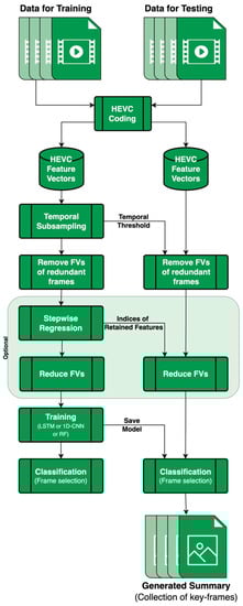
Figure 1.
General overview of the system architecture. Feature extraction is performed through HEVC coding. Temporal subsampling using HEVC features, PCA, or cosine similarity. The reduction of the feature space is optional with stepwise regression. Training is performed with LSTM networks, 1D-CNNs, or random forests.
- The introduction of two new architectures for video summarization based on HEVC features, using LSTM networks and 1D-CNNs.
- The introduction of two new subsampling methods based on cosine similarity and the projections of HEVC feature vectors.
- Complete experimental results with the four most commonly used datasets in video summarization, namely, TVSum, SumMe, OVP, and VSUMM. The use of all four datasets in one research paper rarely occurs in the literature, if at all. From our observations and experimental results, it is rarely the case that a reported video summarization solution works well for all four datasets. Therefore, most papers opt to use a subset of these four datasets.
- A detailed discussion regarding the suitability of different methodologies used in digital video summarization, including accuracy and computational time.
Video summarization has been the subject of substantial research over the past two decades. The efforts made to handle the challenge of video summarization are outlined in this section, with a focus on deep-learning-based approaches.
The authors of [13] took advantage of spatio-temporal learning with 3D-CNNs, LSTMs, and recurrent neural networks to detect soccer video highlights. A GAN-based framework was presented in [14] with an attention-aware Ptr-Net generator and a 3D-CNN discriminator. HEVC intra-frame coding was leveraged by the authors of [15] via merging weighted luminance and chrominance values with a texture-based feature against a threshold to group frames into a video summary. In [16], a stacked memory network (SMN) with LSTM layers was presented that models long dependencies among frames to decrease redundancy in the final summaries. A framework presented in [17] focuses on cost-sensitive learning by having a spatial stream that represents the appearance of frames and a temporal stream that uses motion vectors to represent the temporal information of a video.
The authors of [18] built an unsupervised GAN with an attention mechanism to detect meaningful parts of a video. In [19], motion information between frames is leveraged as spatio-temporal information is extracted and inter-frame motion is generated from it, and a self-attention model selects key frames for the summary. Multi-video summarization was explored by the authors of [20], who applied target-appearance-based shot segmentation in addition to feature extraction from frames; these features were passed to a bidirectional LSTM to generate probabilities to form a summary. An attentive encoder–decoder network was presented by the authors of [21], in which they used a bidirectional LSTM as the encoder to extract contextual information between frames and then two attention-based LSTM networks as the decoder, which used additive and multiplicative objective functions. An encoder–decoder CNN structure was developed by the authors of [22], who used a diagnostic view plane detection network as the encoder, followed by a decoder that feeds features into a bidirectional LSTM to analyze the features of preceding and future frames. The final reinforcement learning network selected key frames for the summary. Video summarization was achieved by the authors of [23] in the Internet of Things (IoT) domain by developing a CNN for shot segmentation and image memorability, using aesthetic- and entropy-based features to ensure summary variation. The work in [24] used motion information and a clustering validity index to segment shots and select key frames by estimating their forward and backward motion.
A self-attention binary neural tree (SABT-Net) model was presented in [25], in which the authors used GoogleNet for feature extraction in addition to shot encoding, branch routing, self-attention, and score prediction modules to achieve video summarization. The authors of [26] used a sparse autoencoder to combine feature vectors derived from multiple pre-trained CNNs into a reduced space with a random forest classifier to form video summaries. A TTH-RNN was presented in [27] and comprised a tensor train embedding layer with a hierarchical LSTM to capture forward and backward temporal intra-shot dependencies and encoded inter-shot dependencies to establish the importance of each frame and form a final summary. The authors of [28] offer CLIP-It, a framework for dealing with query-focused video summarization through the use of a multimodal transformers that correlates frames with user-written queries.
The authors of [29] proposed a deep hierarchical LSTM with attention for video summarization (DHAVS) in response to the LSTM’s inability to handle longer video sequences. They used a 3D-CNN to extract spatio-temporal features and an attention-based hierarchical LSTM module to capture the temporal correlations between video frames. Since most summarizing techniques analyze the visual components of the video and ignore audio elements, the authors of [30] provide a method that uses both visual and audio information. A structural similarity index was used to determine similarity among frames, and the mel-frequency cepstral coefficient was used for feature extraction from audio signals.
The authors of [31] used GANs to extract representative parts of the videos as features through reconstruction loss followed by knowledge distillation, using a basic network for key frame selection. The authors of [32] used a bidirectional LSTM that took advantage of the underlying hierarchical structure of video sequences and learned temporal representations via intra-block and inter-block attention. They then partitioned shots and calculated shot-level importance scores to rank the frames that were included in the final video summary.
2. Methodology
2.1. Data Preprocessing
The original videos were converted into YUV frames before they were encoded using a HEVC/H.265 video coder. We modified the coder to produce low-level features, which are discussed in this section. The HEVC codec is used to compress the videos; hence, rich feature sets can be extracted from it based on the quadratic recursive splitting of the coding units (CUs) in the HEVC. An overview of the process of acquiring the HEVC feature set is shown in Figure 2.
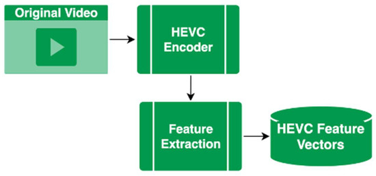
Figure 2.
MPEG to HEVC video conversion process to extract HEVC features.
CUs in HEVC can vary in depth from 0, which is typically equivalent to a maximum block size of 64 × 64 pixels, to 3, which is equivalent to a block of 16 × 16 pixels. The CUs are then split to prediction units (PUs) of a size from 4 × 4 to 32 × 32, which are then further split into transform units (TUs) of a size from 4 × 4 to 32 × 32. Figure 3 illustrates the partitioning scheme followed in HEVC coding. We based our feature vectors on the partitioning and prediction information found in the output bit streams.
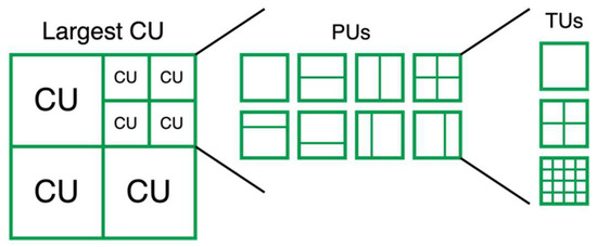
Figure 3.
Coding unit partitioning in HEVC coding.
For video summarization, we presented a set of 64 feature variables. The variables were chosen to quantify the spatio-temporal activity of the video frames. Table 1 presents a list of the variables. The feature variables in Table 1-A are averaged per frame, and the rest in Table 1-B are not. The tables use the abbreviations MVD for motion vector difference, SAD for the sum of absolute differences, and CU for coding unit.

Table 1.
HEVC features extracted per frame from a custom HEVC decoder [8]. (A) Feature variables that are averaged per frame. (B) Feature variables that are not averaged per frame.
These features were chosen as they capture the spatio-temporal activities of the video frames; they also rely on motion estimation and compensation with previous video frames and thus preserve the temporal dependencies.
2.2. Temporal Subsampling
The temporal subsampling of frames is necessary to reduce the amount of video data that must be fed into our proposed models. This is commonly practiced in video summarization as many frames contain redundant content in the temporal sense. In this work, temporal subsampling was carried out through one of the following proposed methods.
2.2.1. HEVC-Based Temporal Subsampling
We used the sum of the HEVC features as an indication of the temporal activity of individual video frames. This can be achieved by summing up all the HEVC feature values to create a temporal activity index. The lower the index, the lower the temporal activity, indicating that the underlying frame is potentially redundant and can be safely deleted. We carried out comprehensive experiments, and we found that the summations of the HEVC feature variables were lower for redundant frames. Conceptually, this is a valid conclusion as the HEVC feature variables mainly rely on motion estimation and compensation, thus capturing the temporal activity of the video frames. Lower summations pertain to redundant frames and vice versa.
In general, the temporal activity index of each frame was compared with a threshold to determine whether it would be deleted.
The calculation of the threshold was based on the training split in each of the five splits in each run. The average values of each and every feature listed in Table 1 were calculated per training split using video frames with a ground truth value of zero (i.e., video frames that were not included in the video summary). This resulted in 64 average values that were summed to generate a “sum of averages”. Likewise, the standard deviations of each and every feature listed in Table 1 were calculated per training split using video frames with a ground truth value of zero. This resulted in 64 standard deviation values that were summed to generate a “sum of standard deviations”. Lastly, the threshold was computed as: “sum of averages” + “sum of standard deviations”. This process is illustrated in Figure 4. To vary the percentage of deleted frames, we added a multiplier to the calculated threshold which had a range of 0 to 1. In this work, using empirical testing, we set the multiplier to 0.3. Consequently, a video frame was retained if its sum of features was greater than the calculated threshold and vice versa.
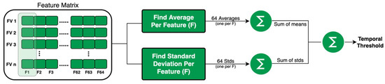
Figure 4.
Calculation of temporal activity threshold for temporal subsampling with HEVC features.
2.2.2. PCA-Based Temporal Subsampling
A principal component analysis (PCA) is a well-known dimensionality reduction method [33]. In our proposed setup, we used a PCA to project each of the feature vectors into a scalar value. Consequently, the consecutive differences of the projected values were computed and stored in list D. Then, for each difference element d in D, we checked it against a threshold and decided whether to retain the underlying video frame. The threshold was based on statistics gathered from the projected feature vector values, as detailed in Algorithm 1.
The theory behind this is that that smaller differences between principal components belonging to feature vectors of frames indicate a higher similarity between them, which indicates redundancy and allows us to remove one of the frames. For example, for the following frames and their feature vectors , the first principle component would appear as , and the consecutive differences would be with and being the differences between and , respectively. In Algorithm 1, with the calculation of the TH, the mean and std are the mean and standard deviation of all values in D, respectively. If is less than the composite thresholding value, then is marked for elimination. This continues until all feature vectors are covered.
This proposed algorithm relies on projecting feature vectors into scalars. The temporal activity threshold is computed based on the means and standard deviations of the differences of these scalar values pertaining to the consecutive feature vectors of a video sequence, hence the use of the first PCA component only.
| Algorithm 1: PCA-based temporal subsampling of frames. |
| Input: FVs_train[]: Feature matrix of train data set FVs_test[]: Feature matrix of test data set k: Predetermined multiplier Output: IDX_DEL[]: Frame indices to delete // Calculate temporal TH [Projected_FVs, first_PC] = Project FVs_train using PCA into scalar values D = Consecutive differences of Projected_FVs mean = Mean of all values in D std = Standard deviation of all values in D TH = // Perform temporal subsampling for each FV in FVs_test do p = Project FV using first_PC if p ≤ TH Append index of FV to IDX-DEL[] end end |
2.2.3. Cosine-Based Temporal Subsampling
Cosine similarity [34] is a metric that assesses how similar two vectors are to one another. It represents the cosine of the angle formed by the two vectors. Cosine similarity is formally defined as the division between the dot product of the vectors and the product of the Euclidean magnitude of each vector. The range of the cosine similarity value is from 0 to 1, with 1 denoting the highest similarity and 0 denoting the lowest. The following is the equation for the cosine similarity score between two feature vectors fi and fj:
In our setup, we applied cosine similarity between each feature vector and its successor, and then stored the similarity score and index of the first feature vector in a tuple list S. After gathering all the similarity scores, the tuple list S was sorted ascendingly. All the feature vectors denoted by scores in the upper 90% (i.e., the scores closer to 1) in the tuple list S were marked for elimination. This subsampling process is detailed in Algorithm 2.
| Algorithm 2: Cosine-based temporal subsampling of frames. |
| Input: FVs[]: Feature matrix of train and test data sets Output: IDX_DEL[]: Frame indices to delete Scores{}: Empty tuple to hold cosine scores for i = 0…count_of(FVs)-1 do C = Cosine score between FVs(i,:) and FVs(i + 1,:) Append [C, i] to Scores {} end Sort Scores{} ascendingly (based on C values) IDX_DEL[] = Indices (i) of upper 90th percentile in Scores{} |
The concept here is that higher similarity scores between feature vectors imply a higher degree of similarity between them, which indicates redundancy and allows the algorithm to eliminate one of the frames. For example, if we have the frames and their feature vectors: , the cosine similarity scores between them are with and being the scores between and , respectively. If is in the upper 90% of the similarity indices then , which is represented by , is marked for elimination, and this continues until all feature vectors are covered.
2.3. Reducing the Feature Space
A supervised feature selection approach known as stepwise regression is used to automatically select the most relevant predictor variables used to predict response variables [35]. The authors of [36] first suggested using stepwise regression in video-based intelligent systems. Since then, it has been effectively employed in many vision-based applications, as documented in several works, including [12,37,38].
In this study, we used stepwise regression to reduce the dimensionality of our feature vectors, where features were treated as predictors and the class labels were treated as response variables. This was carried out to assess the suitability of the selected features and consequently reduce the dimensionality of the feature vectors if needed. Stepwise regression was only used with the training data because it is a supervised approach. Later, the dimensionality of the test data was reduced by using the indices of the retained feature variables of the training set, as illustrated in Figure 5.

Figure 5.
General overview of feature space reduction with stepwise regression.
For completeness, a summary of the stepwise regression algorithm is as follows: for a feature set of , is the F-random feature for the feature to be added to the reduced feature space, and is the feature to be dropped from the reduced feature space. The steps for stepwise regression are as follows:
- 1.
- Create single-set models from all features:where is the hypothesis that the added features are important for classification. was one of the features that yielded the highest F-score. is the statistic of , and is given by the following formula:where is the mean square error, and is the regression sum square error.
- 2.
- Repeat step 1 for all feature variables. For every new h(x) produced, it is examined in combination with the existing h(x) if they produce a higher hypothesis than the older alone. We add if its is greater than and obtain the following:
After adding , is checked for removal by comparing to the new . If is lesser, then is dropped.
- 3.
- The algorithm continues until there are no features to add or drop, with the final hypothesis appearing similar to the following:
2.4. Video Summarization Architectures
2.4.1. LSTM-Based Architecture
Recurrent neural networks (RNNs) [39] are a type of neural network used with sequential or time series data. They differ from standard neural networks, which assume that inputs and outputs are independent, in that they remember information from earlier inputs and use it to impact the current input and output. A major drawback of RNN networks is that they are susceptible to the vanishing gradient problem [40]. The gradient of the loss function approaches zero as the network’s number of layers with activation functions increases, making the network more challenging to train. Due to the vanishing gradient problem, RNNs are not able to remember long-term dependencies. A long short-term memory network (LSTM) is an advanced RNN network that allows information to persist [6]. It is capable of handling the vanishing gradient problem with a chain structure that contains memory blocks called cells.
These cells can forget information that is no longer useful before passing it to the next cell. The output of one cell is taken as input of another. This chain structure is what allows the LSTM to retain only the useful information without suffering from the vanishing gradient problem. The LSTM network can remember the information between different frames of the video while only retaining the important information.
The LSTM architecture used in this work was a four-layer LSTM network with 50 nodes in each layer. The proposed LSTM architecture is shown in Figure 6 (left).
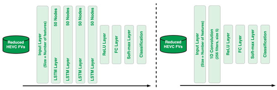
Figure 6.
Proposed LSTM network architecture (left), and 1D-CNN network architecture (right).
2.4.2. One-Dimensional-CNN-Based Architecture
Convolutional neural networks (CNNs), as opposed to conventional artificial neural networks, can combine feature extraction and classification into a single learning body, averting the need for fixed and manually constructed features. In a typical two-dimensional CNN, the kernel can slide along two dimensions of the data [5]. A kernel is a matrix of weights that extracts key information by multiplying them by the input. Contrary, in one-dimensional CNN (1D-CNN), the kernel slides along one dimension of the data in which the convolution operation is applied, significantly reducing the computational complexity.
One-dimensional CNNs are usually used with sequential data due to their simplicity and effectiveness, which is why the architecture used in this work is a single-layer 1D-CNN with 256 filters of size 5. Figure 6 (right) shows the proposed 1D-CNN architecture.
2.4.3. Random-Forest-Based Architecture
The random forest algorithm is a supervised learning approach. An ensemble of decision trees, or a “forest”, are usually trained using the “bagging” method. The fundamental concept of the bagging method is that the final output is improved by combining several learning models [4]. Random forests increase the model’s randomness while creating the decision trees. When splitting a node, it looks for the strongest feature among a random group of features rather than the best feature from the entire set. There is significant variety as a result, which usually results in a better overall model. By using random thresholds for each feature, random forests make trees even more random, as opposed to searching for the best thresholds (such as in conventional decision trees). We employed a threshold of 0.9 in our implementation in order to keep features with values over the threshold. When none of the features were higher than the threshold, they were then all used. For training across the chosen features, we specified that the forest produced 128 trees. Then, in order to quantify the findings, we computed a few performance measures using the predicted labels that we had previously saved.
3. Experimental Results
This section may be divided by subheadings. It should provide a concise and precise description of the experimental results, their interpretation, as well as the experimental conclusions that can be drawn.
3.1. Datasets
In this work, the proposed solutions are evaluated using four popular datasets for video summarization, namely, TVSum [41], SumMe [42], OVP [43], and VSUMM [43]. The TVSum dataset contains 50 videos of various genres such as news, documentaries, and vlogs at 30 fps. The SumMe dataset contains 25 videos at 30 fps. The OVP (Open Video Project) dataset has 50 videos of several genres from the Open Video Project, presented at 30 and with a duration of 1–4 min. The VSUMM dataset contains 50 videos from YouTube, also from several genres, provided at 30 fps with a duration of 1–10 min.
In these datasets, video summaries are generated manually by a number of users and stored in a matrix referred to as “user summaries” which is used as the ground truth. Some existing research papers clearly state that they compare their automatically generated summaries against each of the user summaries and report the average F-score, while other research papers loosely mention that their automatically generated summaries are compared against the ground truth without further details.
Since this work was concerned with static video summarization or key frame extraction, we trained and tested the datasets on the disjunction (inclusive OR) of all user summaries. In our published datasets, we refer to these vectors as “user_summary_inclusive_OR”, which we added to the files of the datasets and made publicly available.
To the best of our knowledge, the use of all four datasets in one research paper rarely occurs in the reporting of experimental results in the literature. From our observations and experimental results, it is rarely the case that a reported video summarization solution works well on all four datasets. Therefore, most papers opt to use a subset of these four datasets.
3.2. Evaluation Criteria
We used quantitative metrics similar to the criteria used in other works for a fair comparison. We define the following metrics using the temporal overlap between the predicted summary A and the ground truth summary B:
To put these metrics into words: precision (P) is the percentage of true positive predictions over all positive predictions, recall (R) is the percentage of true positive predictions over the ground truth, and the F-score (F) is the harmonic mean between them.
3.3. Experimental Setup
Before presenting the results, we describe the general setup that is common to all three proposed architectures. After the video coding feature vectors are generated and the temporal subsampling algorithm is applied, the feature vectors are split in a 20–80% fashion for testing and training, respectively. We apply cross-validation with five folds (K = 5) in which, in every fold, the new testing set shifts by 20% and the older testing set is added back to the training set. The results are then averaged over five folds. The training setup is illustrated in Figure 7.
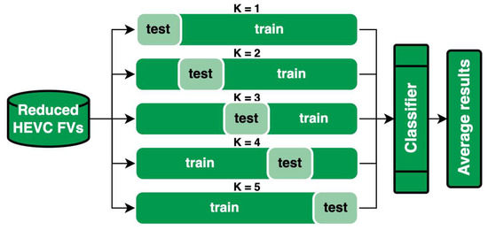
Figure 7.
General overview of learning architecture with averaged results over five folds of cross-validation.
We use HEVC features derived from the custom re-encoder mentioned in Section III. We test our setups with and without a dimensionality reduction of the feature space. In addition, the proposed temporal subsampling of video frames methods using HEVC features, PCA projections, and cosine similarity are all tested with the following three learning architectures: 1D-CNNs, LSTM networks and random forests. For each of the four datasets, the top-performing model from each learning architecture is shortlisted and compared against benchmark methods in the literature. First, the results are reported for every dataset, and the best models are then compared with the literature, followed by a thorough discussion of the results.
The metrics used for comparison are precision (P), recall I and the F-score. The experiments were conducted on a PC with 9th gen Intel i9, 32 GB of RAM, and an NVIDIA RTX 2070 GPU.
3.4. Results
3.4.1. TVSum Dataset
The best results across all learning architectures in Table 2-A do not use stepwise regression (denoted as SW in the tables), while the second-best results do use it for the dimensionality reduction of the feature space. HEVC-based temporal subsampling achieves the highest results in the TVSum dataset, regardless of using stepwise regression or not. The highest overall scores appear with the use of the LSTM network.
Table 2.
Proposed solutions: F-scores of the two best-performing models using the three proposed learning architectures, with and without the reduction of the feature space, and across the three proposed temporal subsampling methods on the TVSum (A), SumMe (B), OVP (C), and VSUMM (D) datasets. Bold scores indicate the highest and underlined scores indicate the second highest.
3.4.2. SumMe Dataset
Regardless of the temporal subsampling method used, all results in the SumMe dataset in Table 2-B are without stepwise regression. Across all learning architectures, the best model uses HEVC-based temporal subsampling, and the second-best model uses PCA-based temporal subsampling. The highest overall scores appear with the use of the random forest architecture.
3.4.3. OVP Dataset
Across all three learning architectures in Table 2-C, the best results in the OVP dataset come from using HEVC-based temporal subsampling and without applying stepwise regression. The second-best model across all learning architectures, however, uses stepwise regression for the dimensionality reduction and cosine similarity for temporal subsampling. The highest overall score appears with the use of the LSTM network.
3.4.4. VSUMM Dataset
In Table 2-D for the VSUMM dataset, all results across all three learning architectures use HEVC-based temporal subsampling. The first across all learning architectures is without stepwise regression, while the second is with stepwise regression. The highest overall scores are with the use of random forests.
3.4.5. All Datasets Versus Benchmarks
Again, as mentioned above, we carried out training and testing using all user summaries combined into one label vector. In the existing work, different papers used different approaches for training and testing, with some of them loosely using the term ground truth without further details. Nonetheless, for completeness, in this section, we provide comparisons against the existing work which carry out training and testing using different approaches but with the same datasets.
Table 3 (A–D) contain the F-scores of our best-performing models from each learning architecture compared against state-of-the-art works in the literature on the SumMe, TVSum, OVP, and VSUMM datasets. With the SumMe dataset in Table 3-A, our random forest model with no dimensionality reduction and with HEVC-based temporal subsampling surpasses the highest scores in the literature.
Table 3.
F-scores of our best performing models from the three proposed learning architectures against benchmark models in the literature on the TVSum (A), SumMe (B), OVP (C), and VSUMM (D) datasets. Sorted ascendingly from top to bottom. Bold scores indicate the highest and underlined scores indicate the second highest.
With the TVSum dataset in Table 3-B, our LSTM network model with no dimensionality reduction and with HEVC-based temporal subsampling also exceeds the highest scores in the literature. Our second- and third-best models with random forests and 1D-CNNs, without dimensionality reduction and with the HEVC-based temporal subsampling of frames, also exceed the benchmark scores.
With the OVP dataset in Table 3-C, our model with the LSTM network without dimensionality reduction and with the HEVC-based temporal subsampling of frames surpasses the highest scores in the literature. Our second- and third-ranking models with random forests and 1D-CNNs, without dimensionality reduction, and with HEVC-based temporal subsampling also outperform the benchmark scores.
With the VSUMM dataset in Table 3-D, our model with random forests, without using stepwise regression, and with HEVC-based temporal subsampling tops the best scores in the literature. Our second- and third-best models with LSTM networks and 1D-CNNs, without stepwise regression and with the HEVC-based temporal subsampling of frames, also exceed benchmark scores.
4. Discussion of Results
4.1. Reduction of Feature Space
One observation from the results in Table 2 is that the highest score is constantly achieved without resorting to reducing the dimensionality of the HEVC feature set. Dimensionality reduction methods aim to retain the most representative features and discard the features that are deemed unnecessary, redundant, or non-representative of the original image information. The fact that retaining all and not some of the 64 HEVC features yields higher scores means that all 64 HEVC features are excellent representatives, and none of them can be discarded.
This is also true for the second-highest scores across all learning architectures in the SumMe dataset but with the PCA-based temporal subsampling of frames per training set. This means that for the SumMe dataset, the quality of the features used is more important or influential than the method used for the temporal subsampling of frames due to the difficult nature of the videos it contains, which were intended to be used with importance- and interestingness-based applications of video summarization [52]. According to the presented results, HEVC features successfully capture importance and interestingness information of video frames.
For TVSum, OVP, and VSUMM, the second-highest score across all three learning architectures is achieved when HEVC features are reduced with stepwise regression regardless of the temporal subsampling method used. The interesting finding with the TVSum and VSUMM datasets is that the F-score of the video summarization is negatively affected by less than 2% when the HEVC-based temporal subsampling of frames is used compared to the best scores. Even in the case of the second-highest scores in the OVP dataset, in which dimensionality reduction is applied and cosine similarity is used for temporal subsampling, the decrease in the F-score is less than 2% as well. This indicates that even when some of the HEVC features are removed, regardless of the method being used for temporal subsampling, the retained features are still highly representative of the frame content and contain close and comparable information compared to the full set of HEVC features.
In general, the use of stepwise regression did not generate the best results in any of our experiments. This can be justified by the fact that stepwise regression uses linear multivariate regression for variable selection. However, the problem at hand, which is mapping feature variables to key frames, is clearly non-linear, leading the stepwise regression approach to fail.
The following are examples of using stepwise regression with the TVSum and SumMe datasets. For the TVsum dataset, we found that the most significant features pertain to the following IDs from Table 1: 4, 5, 8, and 9 and standard deviations of (2–4, 6–8), 10–13, 23–25, and 30, and 10 bins of MVx histogram and 12 bins of the MVy histogramm whereas for the SumMe dataset, we found that the most significant features pertain to the following IDs from Table 1: 3 and 5–7, standard deviations of 1 and 4, 23, standard deviations of 23 and 30, and 7 bins of MVx histogram and 5 bins of the MVy histogram.
4.2. Learning Architecture
Recall that the HEVC features are extracted from the HEVC video coding process. Such a process is based on motion estimation and compensation, which is known to make use of previous video frames in the coding of the present video frame. As such, the resultant feature vector of a video frame inherently contains information from previous frames. This justifies the outstanding results obtained using the RF and 1D-CNN architectures which, unlike LSTM networks, lack the ability to maintain information beyond the current frame.
On the other hand, in SumMe and VSUMM, RFs achieved higher scores compared to the other two learning architectures, implying less content or scene changes in the content of the videos within these datasets. When a video contains many scene changes, LSTMs excel; however, when there are not many changes, RFs can keep up with and exceed LSTMs in terms of classification accuracy.
The datasets in which LSTM networks performed better, i.e., TVSum and OVP, indicate that the videos contained in them have more temporal variance or scene changes in their content compared to the other two datasets. This can be explained by the way LSTM networks work; they can retain information about older frames or content through their long memory in addition to the recently preceding frames with their short memory.
4.3. Elapsed Runtimes
LSTM networks are computationally expensive and require at least four times the resources required by 1D-CNNs or random forests, according to our experiments. When runtime is not a priority, LSTM networks are recommended. On the other hand, when runtime is a priority, random forests are the learning architecture of choice. One-dimensional CNNs still have a place when the runtime is of absolute significance and the accuracy of the summary is not highly prioritized or is not intended to be relied upon in a sensitive application. Recall that in this work, we used cross-validation with K = 5 to generate the results; the results reported in the experiment are for both K = 5 and K = 1.
In conclusion, as the proposed feature set contains only 64 variables, the model generation and testing time is very fast in comparison to typical works in which hundreds or thousands of CNN features are used.
5. Limitations and Future Work
This work was designed for key frame extraction or static video summarization; however, we do not know how it can be expanded or modified to work for dynamic video summarization, which is usually a computationally heavier task. For the learning architectures used, LSTM architectures can be a limiting factor due to expensive computation. However, this can be remedied by using alternative architectures, such as light-weight 1D-CNNs and random forests.
In HEVC-based temporal subsampling, we mentioned using a multiplier to vary the mount of deleted or eliminated frames that was arrived at through empirical testing. This multiplier can be potentially calculated dynamically or in an automated manner.
6. Conclusions
In this work, we presented multiple proposals for generating summaries of video content in the form of key frames. The proposals are based on a precise and concise feature set generated from an HEVC video coder. We presented novel methods for the temporal subsampling of frames using PCA projections and cosine similarity, in addition to the use of stepwise regression for the reduction of the feature space.
We also developed three learning architectures using LSTM networks, 1D-CNNs, and random forests. The experimental results section presented extensive results using all four well-known datasets in the video summarization domain, namely, TVSum, SumMe, OVP, and VSUMM. The reported results surpass reviewed work in the literature in terms of their F-scores. The advantage against existing work is mainly attributed to our use of HEVC features that are based on video coding. Such coding is based on motion estimation and compensation, leading the final HEVC feature vectors to successfully capture temporal dependencies across frames. The reported results are not exclusive to high F-scores but also include reasonable runtimes. The feature vectors have a length of 64 features only, making them compact compared to traditional features from well-known pre-trained CNN networks, which have lengths that are usually in the hundreds or thousands of features.
Author Contributions
Conceptualization, O.I. and T.S.; methodology, O.I. and T.S.; software, O.I. and T.S.; validation, O.I. and T.S.; formal analysis, O.I. and T.S.; investigation, O.I. and T.S.; resources, O.I. and T.S.; data curation, O.I. and T.S.; writing—original draft preparation, O.I. and T.S.; writing—review and editing, O.I. and T.S.; visualization, O.I. and T.S.; supervision, O.I. and T.S.; project administration, O.I. and T.S.; funding acquisition, O.I. and T.S. All authors have read and agreed to the published version of the manuscript.
Funding
The work in this paper is supported by the American University of Sharjah under research grant number FRG22-E-E44. The work in this paper was also supported, in part, by the Open Access Program from the American University of Sharjah.
Data Availability Statement
The datasets used are made publicly available via GitHub at: https://github.com/b00071518/HEVC-SVS (accessed on 1 January 2023).
Acknowledgments
This paper represents the opinions of the author(s) and does not mean to represent the position or opinions of the American University of Sharjah.
Conflicts of Interest
The authors declare no conflict of interest.
References
- Basavarajaiah, M.; Sharma, P. Survey of Compressed Domain Video Summarization Techniques. ACM Comput. Surv. 2020, 52, 116. [Google Scholar] [CrossRef]
- Apostolidis, E.; Adamantidou, E.; Metsai, A.I.; Mezaris, V.; Patras, I. Video Summarization Using Deep Neural Networks: A Survey. arXiv 2021, arXiv:2101.06072. [Google Scholar] [CrossRef]
- Van Der Maaten, L.; Postma, E.; Van den Herik, J. Others Dimensionality reduction: A comparative study. J. Mach. Learn. Res. 2009, 10, 13. [Google Scholar]
- Breiman, L. Random Forests. Mach. Learn. 2001, 45, 5–32. [Google Scholar] [CrossRef]
- Szegedy, C.; Liu, W.; Jia, Y.; Sermanet, P.; Reed, S.; Anguelov, D.; Erhan, D.; Vanhoucke, V.; Rabinovich, A. Going Deeper with Convolutions. arXiv 2014, arXiv:1409.4842. [Google Scholar]
- Hochreiter, S.; Schmidhuber, J. Long Short-Term Memory. Neural Comput. 1997, 9, 1735–1780. [Google Scholar] [CrossRef] [PubMed]
- Sullivan, G.J.; Ohm, J.-R.; Han, W.-J.; Wiegand, T. Overview of the High Efficiency Video Coding (HEVC) Standard. IEEE Trans. Circuits Syst. Video Technol. 2012, 22, 1649–1668. [Google Scholar] [CrossRef]
- Issa, O.; Shanableh, T. CNN and HEVC Video Coding Features for Static Video Summarization. IEEE Access 2022, 10, 72080–72091. [Google Scholar] [CrossRef]
- Hassan, M.; Shanableh, T. Predicting split decisions of coding units in HEVC video compression using machine learning techniques. Multimed. Tools Appl. 2019, 78, 32735–32754. [Google Scholar] [CrossRef]
- Shanableh, T. Altering split decisions of coding units for message embedding in HEVC. Multimed. Tools Appl. 2018, 77, 8939–8953. [Google Scholar] [CrossRef]
- Youssef, S.; Shanableh, T. Detecting Double and Triple Compression in HEVC Videos Using the Same Bit Rate. SN Comput. Sci. 2021, 2, 406. [Google Scholar] [CrossRef]
- Shanableh, T. Saliency detection in MPEG and HEVC video using intra-frame and inter-frame distances. Signal Image Video Process. 2016, 10, 703–709. [Google Scholar] [CrossRef]
- Agyeman, R.; Muhammad, R.; Choi, G.S. Soccer Video Summarization Using Deep Learning. In Proceedings of the 2019 IEEE Conference on Multimedia Information Processing and Retrieval (MIPR), San Jose, CA, USA, 28–30 March 2019; pp. 270–273. [Google Scholar] [CrossRef]
- Fu, T.-J.; Tai, S.-H.; Chen, H.-T. Attentive and Adversarial Learning for Video Summarization. In Proceedings of the 2019 IEEE Winter Conference on Applications of Computer Vision (WACV), Waikoloa Village, HI, USA, 7–11 January 2019; pp. 1579–1587. [Google Scholar] [CrossRef]
- Wang, F.; Liu, F.; Zhu, S.; Fu, L.; Liu, Z.; Wang, Q. HEVC intra frame based compressed domain video summarization. In Proceedings of the International Conference on Artificial Intelligence, Information Processing and Cloud Computing, AIIPCC’19, Sanya, China, 19–21 December 2019; ACM Press: New York, NY, USA, 2019; pp. 1–7. [Google Scholar] [CrossRef]
- Wang, J.; Wang, W.; Wang, Z.; Wang, L.; Feng, D.; Tan, T. Stacked Memory Network for Video Summarization. In Proceedings of the 27th ACM International Conference on Multimedia, Nice, France, 21–25 October 2019; ACM: New York, NY, USA, 2019; pp. 836–844. [Google Scholar] [CrossRef]
- Zhong, S.; Wu, J.; Jiang, J. Video summarization via spatio-temporal deep architecture. Neurocomputing 2019, 332, 224–235. [Google Scholar] [CrossRef]
- Apostolidis, E.; Adamantidou, E.; Metsai, A.I.; Mezaris, V.; Patras, I. Unsupervised Video Summarization via Attention-Driven Adversarial Learning. In MultiMedia Modeling; Ro, Y.M., Cheng, W.-H., Kim, J., Chu, W.-T., Cui, P., Choi, J.-W., Hu, M.-C., De Neve, W., Eds.; Lecture Notes in Computer Science; Springer International Publishing: Cham, Switzerland, 2020; Volume 11961, pp. 492–504. ISBN 978-3-030-37730-4. [Google Scholar] [CrossRef]
- Huang, C.; Wang, H. A Novel Key-Frames Selection Framework for Comprehensive Video Summarization. IEEE Trans. Circuits Syst. Video Technol. 2020, 30, 577–589. [Google Scholar] [CrossRef]
- Hussain, T.; Muhammad, K.; Ullah, A.; Cao, Z.; Baik, S.W.; de Albuquerque, V.H.C. Cloud-Assisted Multiview Video Summarization Using CNN and Bidirectional LSTM. IEEE Trans. Ind. Inform. 2020, 16, 77–86. [Google Scholar] [CrossRef]
- Ji, Z.; Xiong, K.; Pang, Y.; Li, X. Video Summarization With Attention-Based Encoder–Decoder Networks. IEEE Trans. Circuits Syst. Video Technol. 2020, 30, 1709–1717. [Google Scholar] [CrossRef]
- Liu, T.; Meng, Q.; Vlontzos, A.; Tan, J.; Rueckert, D.; Kainz, B. Ultrasound Video Summarization Using Deep Reinforcement Learning. In Medical Image Computing and Computer Assisted Intervention—MICCAI 2020: 23rd International Conference, Lima, Peru, 4–8 October 2020; Martel, A.L., Abolmaesumi, P., Stoyanov, D., Mateus, D., Zuluaga, M.A., Zhou, S.K., Racoceanu, D., Joskowicz, L., Eds.; Lecture Notes in Computer Science; Springer International Publishing: Cham, Switzerland, 2020; Volume 12263, pp. 483–492. ISBN 978-3-030-59715-3. [Google Scholar] [CrossRef]
- Muhammad, K.; Hussain, T.; Tanveer, M.; Sannino, G.; de Albuquerque, V.H.C. Cost-Effective Video Summarization Using Deep CNN With Hierarchical Weighted Fusion for IoT Surveillance Networks. IEEE Internet Things J. 2020, 7, 4455–4463. [Google Scholar] [CrossRef]
- Zhao, Y.; Guo, Y.; Sun, R.; Liu, Z.; Guo, D. Unsupervised video summarization via clustering validity index. Multimed. Tools Appl. 2020, 79, 33417–33430. [Google Scholar] [CrossRef]
- Song, J.; He, T.; Gao, L.; Xu, X.; Hanjalic, A.; Shen, H.T. Unified Binary Generative Adversarial Network for Image Retrieval and Compression. Int. J. Comput. Vis. 2020, 128, 2243–2264. [Google Scholar] [CrossRef]
- Nair, M.S.; Mohan, J. Static video summarization using multi-CNN with sparse autoencoder and random forest classifier. Signal Image Video Process. 2021, 15, 735–742. [Google Scholar] [CrossRef]
- Zhao, B.; Li, X.; Lu, X. TTH-RNN: Tensor-Train Hierarchical Recurrent Neural Network for Video Summarization. IEEE Trans. Ind. Electron. 2021, 68, 3629–3637. [Google Scholar] [CrossRef]
- Narasimhan, M.; Rohrbach, A.; Darrell, T. CLIP-It! Language-Guided Video Summarization. arXiv 2021, arXiv:2107.00650. [Google Scholar]
- Lin, J.; Zhong, S.; Fares, A. Deep hierarchical LSTM networks with attention for video summarization. Comput. Electr. Eng. 2022, 97, 107618. [Google Scholar] [CrossRef]
- Rhevanth, M.; Ahmed, R.; Shah, V.; Mohan, B.R. Deep Learning Framework Based on Audio–Visual Features for Video Summarization. In Advanced Machine Intelligence and Signal Processing; Gupta, D., Sambyo, K., Prasad, M., Agarwal, S., Eds.; Lecture Notes in Electrical Engineering; Springer Nature Singapore: Singapore, 2022; Volume 858, pp. 229–243. ISBN 978-981-19083-9-2. [Google Scholar]
- Sreeja, M.U.; Kovoor, B.C. A multi-stage deep adversarial network for video summarization with knowledge distillation. J. Ambient Intell. Humaniz. Comput. 2022. [Google Scholar] [CrossRef]
- Zhu, W.; Lu, J.; Han, Y.; Zhou, J. Learning multiscale hierarchical attention for video summarization. Pattern Recognit. 2022, 122, 108312. [Google Scholar] [CrossRef]
- Jolliffe, I.T.; Cadima, J. Principal component analysis: A review and recent developments. Philos. Trans. R. Soc. Math. Phys. Eng. Sci. 2016, 374, 20150202. [Google Scholar] [CrossRef]
- Singhal, A.; Google, I. Modern Information Retrieval: A Brief Overview. IEEE Data Eng. Bull. 2001, 24, 35–43. [Google Scholar]
- Montgomery, D.C.; Runger, G.C. Applied Statistics and Probability for Engineers; EMEA edition; Seventh edition; Wiley: Hoboken, NJ, USA, 2018; ISBN 978-1-119-40036-3. [Google Scholar]
- Shanableh, T.; Assaleh, K. Feature modeling using polynomial classifiers and stepwise regression. Neurocomputing 2010, 73, 1752–1759. [Google Scholar] [CrossRef]
- Shanableh, T. A regression-based framework for estimating the objective quality of HEVC coding units and video frames. Signal Process. Image Commun. 2015, 34, 22–31. [Google Scholar] [CrossRef]
- Shanableh, T. Detection of frame deletion for digital video forensics. Digit. Investig. 2013, 10, 350–360. [Google Scholar] [CrossRef]
- Abiodun, O.I.; Jantan, A.; Omolara, A.E.; Dada, K.V.; Mohamed, N.A.; Arshad, H. State-of-the-art in artificial neural network applications: A survey. Heliyon 2018, 4, e00938. [Google Scholar] [CrossRef] [PubMed]
- Hochreiter, S. The Vanishing Gradient Problem During Learning Recurrent Neural Nets and Problem Solutions. Int. J. Uncertain. Fuzziness Knowl.-Based Syst. 1998, 6, 107–116. [Google Scholar] [CrossRef]
- Song, Y.; Vallmitjana, J.; Stent, A.; Jaimes, A. TVSum: Summarizing web videos using titles. In Proceedings of the 2015 IEEE Conference on Computer Vision and Pattern Recognition (CVPR), Boston, MA, USA, 7–12 June 2015; pp. 5179–5187. [Google Scholar] [CrossRef]
- Gygli, M.; Grabner, H.; Riemenschneider, H.; Van Gool, L. Creating Summaries from User Videos. In Computer Vision–ECCV 2014: 13th European Conference, Zurich, Switzerland, 6–12 September 2014; Springer: Cham, Switzerland, 2014. [Google Scholar]
- de Avila, S.E.F.; da_Luz, A., Jr.; de A. Araújo, A.; Cord, M. VSUMM: An Approach for Automatic Video Summarization and Quantitative Evaluation. In Proceedings of the 2008 XXI Brazilian Symposium on Computer Graphics and Image Processing, Campo Grande, Brazil, 12–15 October 2008; pp. 103–110. [Google Scholar] [CrossRef]
- Liu, Y.-T.; Li, Y.-J.; Wang, Y.-C.F. Transforming Multi-Concept Attention into Video Summarization. arXiv 2020, arXiv:2006.01410. [Google Scholar]
- Zhu, W.; Han, Y.; Lu, J.; Zhou, J. Relational Reasoning Over Spatial-Temporal Graphs for Video Summarization. IEEE Trans. Image Process. 2022, 31, 3017–3031. [Google Scholar] [CrossRef] [PubMed]
- Wu, J.; Zhong, S.; Jiang, J.; Yang, Y. A novel clustering method for static video summarization. Multimed. Tools Appl. 2017, 76, 9625–9641. [Google Scholar] [CrossRef]
- de Avila, S.E.F.; Lopes, A.P.B.; da Luz, A.; de Albuquerque Araújo, A. VSUMM: A mechanism designed to produce static video summaries and a novel evaluation method. Pattern Recognit. Lett. 2011, 32, 56–68. [Google Scholar] [CrossRef]
- Zhang, K.; Grauman, K.; Sha, F. Retrospective Encoders for Video Summarization. In Computer Vision—ECCV 2018; Ferrari, V., Hebert, M., Sminchisescu, C., Weiss, Y., Eds.; Lecture Notes in Computer Science; Springer International Publishing: Cham, Switzerland, 2018; Volume 11212, pp. 391–408. ISBN 978-3-030-01236-6. [Google Scholar] [CrossRef]
- Apostolidis, E.; Balaouras, G.; Mezaris, V.; Patras, I. Combining Global and Local Attention with Positional Encoding for Video Summarization. In Proceedings of the 2021 IEEE International Symposium on Multimedia (ISM), Naple, Italy, 6–8 December 2021; pp. 226–234. [Google Scholar] [CrossRef]
- Mussel Cirne, M.V.; Pedrini, H. VISCOM: A robust video summarization approach using color co-occurrence matrices. Multimed. Tools Appl. 2018, 77, 857–875. [Google Scholar] [CrossRef]
- Feng, L.; Li, Z.; Kuang, Z.; Zhang, W. Extractive Video Summarizer with Memory Augmented Neural Networks. In Proceedings of the 26th ACM International Conference on Multimedia, Seoul, Republic of Korea, 22–26 October 2018; ACM: New York, NY, USA, 2018; pp. 976–983. [Google Scholar] [CrossRef]
- Atencio, P.; German, S.; Branch, J.W.; Delrieux, C. Video summarisation by deep visual and categorical diversity. IET Comput. Vis. 2019, 13, 569–577. [Google Scholar] [CrossRef]


Disclaimer/Publisher’s Note: The statements, opinions and data contained in all publications are solely those of the individual author(s) and contributor(s) and not of MDPI and/or the editor(s). MDPI and/or the editor(s) disclaim responsibility for any injury to people or property resulting from any ideas, methods, instructions or products referred to in the content. |
© 2023 by the authors. Licensee MDPI, Basel, Switzerland. This article is an open access article distributed under the terms and conditions of the Creative Commons Attribution (CC BY) license (https://creativecommons.org/licenses/by/4.0/).